Research on high-resolution processing of frequency modulation combined signal for active sonar detection

The Frequency Modulation Combined (FMC) waveform has delay (range)-Doppler (velocity) coupling resolution, and the traditional nonlinear high-resolution algorithms represented by Point-wise Product (PP) and Point-wise Minimization (PM) have good anti-reverberation performances, but their detection performances are poor under low Signal-to-Noise Ratio (SNR) conditions. We propose the improved method PAMP by combining PP and PM methods, and select the combination waveform of “W”-type Linear Frequency Modulation (W-LFM) as the processing object, verifying the effectiveness of the proposed method through numerical simulation and lake experiment. Firstly, the ROC curve analysis shows that the detection performance of PAMP is significantly improved compared with PM and PP, and is close to the optimal detector. Secondly, numerical simulation shows that PAMP is more suitable for target detection in low SNR scenario, where it has a narrower resolution width and lower reverberation energy. Finally, we design lake experiment and analyze the data processing results. The active sonar display image in direction-velocity-range coordinates demonstrates the high-resolution advantage of the FMC signal represented by W-LFM. Moreover, PAMP effectively reduces the intensity of reverberation area and improves the range-velocity resolution, realizing the high-resolution detection for active sonar.

1 Introduction

In the field of radar and sonar, the Matched Filter (MF) is defined as the best receiver of active signals because it is a linear filter with maximum output Signal-to-Noise Ratio (SNR) [1–3]. The Ambiguity Function (AF) based on the output response of the MF portrays the delay (range) and Doppler (velocity) resolution characteristics of signal and is an indispensable method for active sonar waveform design and signal processing [4–6]. Frequency Modulation (FM) waveforms such as Linear FM (LFM) and Hyperbolic FM (HFM) commonly used in active sonar have good Doppler tolerance, which is conducive to signal detection, but the two-dimensional delay-Doppler coupling resolution is poor, which makes it impossible to accurately estimate the range and velocity [7–9].

Reverberation is one of the main factors interfering with active sonar detection and is most evident in shallow water [10, 11]. A large number of scattered waves from the seabed and sea surface enter the active sonar system and degrade the target detection and discrimination performance [12–14]. In terms of ambiguity function shape, the main lobes of the pegboard [15–17] and thumbtack [18–20] signals are high-resolution, which is advantageous in single-target detection under ideal conditions [21–23]. However, subject to the limitation of constant ambiguity volume [24], higher sidelobes or bases in noisy or reverberant backgrounds can cause interference in the detection and discrimination of multiple targets. Although there are several waveform optimization schemes available in the radar and sonar fields, there is no corresponding special high-resolution processing method to reduce the reverberation output [25–27]. Therefore, the design of a high-resolution active transmit waveform with high transmit efficiency and low sidelobe and the corresponding high-resolution signal processing algorithm is the key to the performance of active sonar [28–30].

The FM Combined (FMC) waveform was originally derived from bionic signals [31–33] and consists of multiple FM waveforms. The ambiguity function shape of FMC waveform is characterized by both thumbtack-type and oblique ridge-type features, where multiple oblique ridges cross each other and are superimposed at the coordinate origin to form a thumbtack-type main peak with high delay-velocity resolution. In the multi-target case, due to the intersection and superposition of ridges between different targets, not only the base is elevated, but also a large number of false target peaks will appear, causing interference to the target detection. The conventional processing based on matched filter cannot meet the demand of high-resolution detection. Rasool [34] introduced nonlinear algorithms for ambiguity function processing of radar V-chirp signals, which effectively eliminated the peak ridges and realized the high delay-velocity resolution. Zhu [35, 36] proposed double V-chirp waveform for false target problem under multi-target conditions, which reduces the height of ridges and the incidence of false target. The ridge suppression and high delay-velocity resolution are also realized after nonlinear algorithm processing. Lou [37] introduced the idea of combined waveform design and nonlinear signal processing in radar system into active sonar system, which realized the high delay-velocity resolution and anti-reverberation of active sonar. However, due to the low SNR of hydroacoustic signals, the loss of SNR gain caused by nonlinear processing has a greater impact on the underwater target detection.

The rest of the paper is organized as follows. In section 2, we introduce the FMC waveform model and the concept of its AF. In Section 3, we introduce the nonlinear high-resolution processing and propose an improved method, Point-wise Addition-Minimum-Product (PAMP). The detection performance defects of the existing nonlinear methods and the enhancement of the PMAP are comparatively analyzed by ROC curves. In Section 4, we comparatively analyze the performance advantages of the PMAP by numerical simulation result. In Section 5, we process the experimental data and verify the feasibility of the W-LFM waveform and the high-resolution and anti-reverberation performance of the PMAP. Finally, in Section 6, we summarize the work of this paper and give an outlook for future work.

2 Theoretical framework for frequency modulation combined waveform

2.1 Signal model

The FMC waveform consists of $N_s$ FM sub-waves, which have the same pulse width and can have different bandwidths. The initial and cutoff frequencies of the sub-waves are set according to the waveform design requirements. The ith sub-wave of the FMC waveform is defined as Equation 1.

${\mathit{s}}_{\mathit{i}}\left(\mathit{t}\right)=\mathbf{exp}\left\{\mathit{j}{\mathit{\phi }}_{\mathit{i}}\left[\mathit{t}-\left(\mathit{i}-\mathbf{1}\right){\mathit{T}}_{\mathit{s}}\right]\right\},\left(\mathit{i}-\mathbf{1}\right){\mathit{T}}_{\mathit{s}}\le \mathit{t}\le \mathit{i}{\mathit{T}}_{\mathit{s}}(1)$

Here, $T$ is the total pulse width of the FMC waveform, $T_s$ is the pulse width of the sub-waves, and ${\phi }_i\left(t\right)$ is the instantaneous phase of the ith sub-wave. The FMC waveform can be represented as

$\mathit{s}\left(\mathit{t}\right)={\displaystyle \sum _{\mathit{i}=\mathbf{1}}^{{\mathit{N}}_{\mathit{s}}}}\mathbf{\text{rect}}\left[\frac{\mathit{t}-\left(\mathit{i}-\mathbf{1}\right){\mathit{T}}_{\mathit{s}}}{{\mathit{T}}_{\mathit{s}}}\right]{\mathit{s}}_{\mathit{i}}\left(\mathit{t}\right),\mathbf{0}\le \mathit{t}\le \mathit{T}(2)$

where $N_s$ is the number of sub-waves, $1<i<N_s$, $T_s=T/N_s$. Function $\text{rect}\left(t\right)$ is defined as Equation 3.

$\mathbf{\text{rect}}\left(\mathit{t}\right)=\left\{\begin{array}{l}\mathbf{1},\mathbf{0}\le \mathit{t}\le \mathbf{1}\\ \mathbf{0},\mathbf{\text{others}}\end{array}\right.(3)$

Each sub-waves of the FMC waveform maintains the same pulse width, which is to keep the same SNR gain in sub-wave detection and nonlinear processing. In order to obtain a rational distribution state of ridge lines, the time-frequency curves of the sub-waves can be flexibly adjusted within a given frequency range according to the waveform design needs.

Increasing the number of sub-waves can effectively reduce the false target probability, and the combination of 4 sub-waves is the best choice. We discussed the design and application of “W” type LFM (W-LFM) waveform in our previous work [38], and its time-frequency curve is shown in Figure 1A.

Figure 1

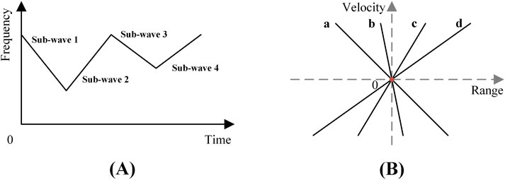
Figure 1. (A) Time-frequency curve of W-LFM waveform. (B) Auto ambiguity function shape of W-LFM waveform.

2.2 Ambiguity function

Both waveform design and signal processing of FMC depend on the performance of its AF. In this paper, we assume a point-target signal model in a Gaussian white noise background [39, 40]. Under this assumption, the target echo is the result of the original waveform after time delay and Doppler spreading. $H_1$ is the target assumption and $H_0$ is the no-target assumption. The received signal can be represented as Equation 4.

${\mathbf{s}}_{\mathit{r}}\left(\mathit{t}\right)=\left\{\begin{array}{l}\mathit{a}\mathit{s}\left[\mathit{k}\left(\mathit{t}-\mathit{\tau }\right)\right]+\mathit{n}\left(\mathit{t}\right),\mathit{u}\mathit{n}\mathit{d}\mathit{e}\mathit{r}{\mathit{H}}_{\mathbf{1}}\\ \mathit{n}\left(\mathit{t}\right),\mathit{u}\mathit{n}\mathit{d}\mathit{e}\mathit{r}{\mathit{H}}_{\mathbf{0}}\end{array}\right.(4)$

Here, $a$ denotes the amplitude and $\tau$ denotes the time delay of target. $k$ denotes the Doppler spreading factor and is defined as $k=\left(c–v\right)/\left(c+v\right)$, where $v$ denotes the target velocity and $\mathrm{c}$ denotes the sound velocity. $n\left(t\right)$ denotes the 0-mean Gaussian white noise. Then the target distance $r=\tau c/2$.

The cross AF and cross sub-AF of received signal are defined respectively as Equation 5.

$\begin{array}{c}\mathit{A}\left(\mathit{\tau },\mathit{v}\right)={\int }_{-\mathit{\infty }}^{+\mathit{\infty }}{\mathit{s}}_{\mathit{r}}\left(\mathit{t}\right){\mathit{s}}^{*}\left[\mathit{k}\left(\mathit{t}-\mathit{\tau }\right)\right]\mathit{d}\mathit{t}\\ {\mathit{A}}_{\mathit{i}}\left(\mathit{\tau },\mathit{v}\right)={\int }_{-\mathit{\infty }}^{+\mathit{\infty }}{\mathit{s}}_{\mathit{r}}\left(\mathit{t}\right){{\mathit{s}}_{\mathit{i}}}^{*}\left\{\mathit{k}\left[\mathit{t}-\left(\mathit{i}-\mathbf{1}\right){\mathit{T}}_{\mathit{s}}-\mathit{\tau }\right]\right\}\mathit{d}\mathit{t}\end{array}(5)$

where “(⋅)^*” denotes the conjugate operation. Substituting Equation 2, we get

$\mathit{A}\left(\mathit{\tau },\mathit{v}\right)={\displaystyle \sum _{\mathit{i}=\mathbf{1}}^{{\mathit{N}}_{\mathit{s}}}}{\mathit{A}}_{\mathit{i}}\left(\mathit{\tau },\mathit{v}\right)(6)$

Since delay and distance have a unique correspondence, cross AF and cross Sub-AF can also be notated: $A\left(r,v\right)$ and $A_i\left(r,v\right)$。

Under the assumption of $H_1$, the cross AF and cross sub-AF can also be called the auto AF and the auto sub-AF when $n\left(t\right)$ = 0, ${\tau }_0$ = 0 and $v_0$ = 0. The auto AF shape of the FM waveform shows oblique ridge-type, and we refer to its centerline as the ridge line in this paper. It can be proved that in the low-velocity range, the ridge lines of FM waveforms are approximately straight lines. From Equation 6, the auto ambiguity function shape of the FMC waveform has $N_s$ superimposed ridge lines.

Figure 1B shows the schematic of the auto AF shape of the W-LFM waveform, which consists of four intersecting ridge lines. The slope of the ridge line of the ith sub-wave $s_i\left(t\right)$ is expressed as [38]

${\mathit{l}}_{\mathit{i}}=\frac{\mathbf{\Delta }\mathit{v}}{\mathbf{\Delta }\mathit{\tau }}=\frac{\mathit{N}\mathbf{c}}{\mathbf{2}\mathit{T}}\frac{{\mathit{f}}_{\mathit{E},\mathit{i}}-{\mathit{f}}_{\mathit{I},\mathit{i}}}{{\mathit{f}}_{\mathit{E},\mathit{i}}+\left({\mathit{f}}_{\mathit{E},\mathit{i}}-{\mathit{f}}_{\mathit{I},\mathit{i}}\right)\left(\mathit{i}-\mathbf{1}\right)}(7)$

where $f_{I,i}$ and $f_{E,i}$ are the initial and cutoff frequencies of $s_i\left(t\right)$, respectively. Equation 7 represents the time-frequency distribution characteristics of the ridge lines, which can guide the FMC waveform design.

The Q-function is defined as the integral of the square of ambiguity function along the delay axis, and is often used to analyze the anti-reverberation properties of a waveform. The expression for the Q-function is [41] is as Equation 8.

$\mathit{Q}\left(\mathit{v}\right)={\int }_{-\mathit{\infty }}^{+\mathit{\infty }}{\left|\mathit{A}\left(\mathit{\tau },\mathit{v}\right)\right|}^{\mathbf{2}}\mathit{d}\mathit{\tau }(8)$

The lower the value of Q-function is, the lower the output energy of the ambiguity function is, indicating the higher anti-reverberation performance of the waveform.

FMC waveform design requires a comprehensive trade-off between the number of sub-waves and the FM parameters, which are related to the distribution of sub-wave ridge lines, thus affecting the resolution performance of the waveform. From the perspective of high-resolution and anti-reverberation, too small an angle between ridge lines will cause mutual interference. From the point of view of false target suppression, the number of sub-waves should be as large as possible. But the increase in the number of sub-waves will not only increase the difficulty of waveform design, but also unfavorable to nonlinear processing.

3 High-resolution processing

High-resolution algorithms based on nonlinear processing greatly reduce the ambiguity function volume of FMC signal, which is an effective approach to realize anti-reverberation, while existing high-resolution algorithms have the disadvantage of large loss of detection performance. In this section, the Point-wise Addition-Minimum-Product (PAMP) is proposed and its improvement in detection performance is analyzed with ROC curves.

3.1 High-resolution receiver

From Equation 6, the ambiguity function of the FMC signal is equivalent to the point-wise summation of $N_s$ sub-AFs, i.e., the conventional MF method. If some nonlinear methods are utilized to preserve the overlapping regions and eliminate the non-overlapping regions of the ridges in the ambiguity function shape, the output ambiguity function shape behaves as a thumbtack shape, which further reduces the output energy on the basis of high-resolution. We refer to this process as high-resolution processing, and a schematic diagram of the high-resolution receiver for FMC signals is shown in Figure 2, where sub-wave AF indicates the sub-wave detection based on MF for the received signal, and nonlinear processing indicates the fusion of the sub-AFs.

Figure 2

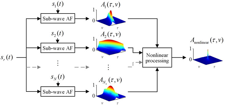
Figure 2. The schematic diagram of the high-resolution receiver.

In the coordinate region where the ridges cross, all sub-AF shapes behave as peaks, and the ambiguity function shape after nonlinear processing remains as peaks. In the coordinate region where the ridges do not cross, at most 1 sub-AF shape behaves as peak while the rest behaves as base, and the ambiguity function shape after nonlinear processing behaves as base. Compared to MF, the ridges are preserved at target coordinates and suppressed at non-targets coordinates in the high-resolution AF shape, which can reduce reverberation on the basic of high-resolution.

Rasool and Zhu [34, 35] describes various nonlinear processing algorithms, each of them has its own advantages and disadvantages, and all of them achieve high-resolution and anti-reverberation at the expense of detection performance. Point-wise Product (PP) has the expression as Equation 9.

${\mathit{A}}_{\mathbf{\text{PP}}}\left(\mathit{\tau },\mathit{v}\right)={\prod }_{\mathit{i}=\mathbf{1}}^{{\mathit{N}}_{\mathit{s}}}\left|{\mathit{A}}_{\mathit{i}}\left(\mathit{\tau },\mathit{v}\right)\right|(9)$

Point-wise product increases the dynamic range of the output image, and its degree of variation increases with the increase in the number of sub-waves. In multi-target scenes, it makes strong targets stronger and weak targets weaker, which is not conducive to comparative analysis and target extraction. To offset the adverse effects caused by changes in dynamic range, we generally take the $N_s$-th square root of $A_{\text{PP}}\left(\tau ,v\right)$ to maintain the original mapping relationship of the output data. Point-wise Minimum (PM) has the expression as Equation 10.

${\mathit{A}}_{\mathbf{\text{PM}}}\left(\mathit{\tau },\mathit{v}\right)=\mathbf{min}\left\{\left|{\mathit{A}}_{\mathit{i}}\left(\mathit{\tau },\mathit{v}\right)\right||\mathbf{1}\le \mathit{i}\le {\mathit{N}}_{\mathit{s}}\right\}(10)$

Here “min{ }” means to find the minimum of the set. Both PP and PM realize high-resolution processing by fusing sub-AFs, and the SNR gain of sub-wave detection is $1/N_s$ of the overall detection gain, resulting in low detection performance of existing nonlinear high-resolution processing.

Monte Carlo method is used to simulate the ROC curves of the signal processing algorithms. The constant false alarm probability is 0.01 and the number of calculations is 100,000. The time bandwidth product of FMC waveforms is 1,000. The ROC curves of PM and PP are shown in Figures 3A, B, respectively, where $N_s$ denotes the number of sub-waves, and as the number of sub-waves increases, the SNR required for detection also increases, i.e., the detection performance decreases. When the number of sub-waves is the same, the detection performance of PM decreases more than that of PP. Therefore, the existing nonlinear high-resolution algorithms have a large loss of detection performance and are not applicable to hydroacoustic target detection.

Figure 3

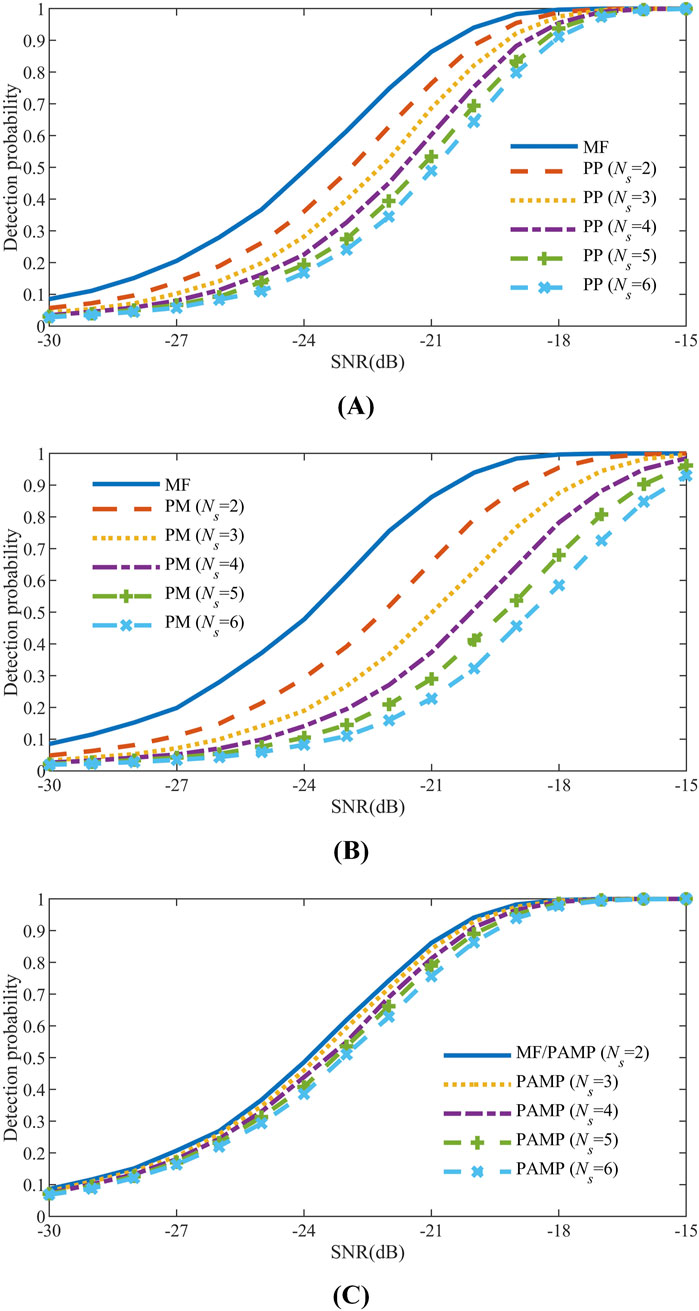
Figure 3. (A) ROC curves of PP. (B) ROC curves of PM. (C) ROC curves of PAMP.

3.2 The PAMP algorithm

In order to improve the detection performance of existing nonlinear methods, this paper proposes an improved method PAMP based on PM and PP. The method reorganizes the sub-wave detection results and improves the SNR gain of individual detection parts without losing the variability of the ambiguity functions, which not only ensures the high-resolution effect but also improves the overall detection performance of the algorithm.

The processing flow of PMAP is shown in Figure 4. First, we add the two sub-AFs point-wise to get Equation 11.

${\mathit{A}}_{\mathit{i},\mathit{j}}\left(\mathit{\tau },\mathit{v}\right)={\mathit{A}}_{\mathit{i}}\left(\mathit{\tau },\mathit{v}\right)+{\mathit{A}}_{\mathit{j}}\left(\mathit{\tau },\mathit{v}\right)(11)$

Figure 4

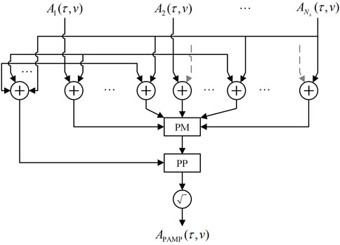
Figure 4. Processing flow of the PAMP.

Here, $1\le i,j\ge N_s$ and $i<j$. $A_{i,j}\left(\tau ,v\right)$ is formed by summing two crossed ridges, and they remain distinct from each other, which provides a basis for nonlinear processing. Disregarding the case of repeated combinations, the number of reconfigured sub-AFs is as Equation 12.

${\mathit{N}}_{\mathbf{\text{rec}}}=\frac{{\mathit{N}}_{\mathit{s}}\left({\mathit{N}}_{\mathit{s}}-\mathbf{1}\right)}{\mathbf{2}}(12)$

Taking the W-LFM waveform as an example, there are six ($i$, $j$) reconfiguration schemes, namely (1, 2), (1, 3), (1, 4), (2, 3), (2, 4), (3, 4). It is worth mentioning that the SNR of reconfigured sub-AFs is twice that of a single sub-AF, but they are not completely independent of each other.

Second, we take a PM of the reconfigured sub-AFs to get.

${\mathit{A}}_{\mathbf{r}\mathbf{e}\mathbf{c}\_\mathbf{P}\mathbf{M}}\left(\mathit{\tau },\mathit{v}\right)=\mathbf{min}\left\{\left|{\mathit{A}}_{\mathit{i},\mathit{j}}\left(\mathit{\tau },\mathit{v}\right)\right||\mathbf{1}\le \mathit{i},\mathit{j}\le {\mathit{N}}_{\mathit{s}}\right\}(13)$

Because of the variability in ridge distribution in reconfigured sub-AFs, the ambiguity function shape for this step behaves as thumbtack shapes similarly to the conventional PP and PM. At last, in order to further enhance the target peak and suppress the base in ambiguity function shape, we multiply Equation 6 and Equation 13 and take the square root to get Equation 14.

${\mathit{A}}_{\mathbf{\text{PAMP}}}\left(\mathit{\tau },\mathit{v}\right)={\left[\mathit{A}\left(\mathit{\tau },\mathit{v}\right)\cdot {\mathit{A}}_{\mathbf{r}\mathbf{e}\mathbf{c}\_\mathbf{P}\mathbf{M}}\left(\mathit{\tau },\mathit{v}\right)\right]}^{\frac{\mathbf{1}}{\mathbf{2}}}(14)$

This step is based on the conventional ambiguity function with the highest SNR gain, and the high-resolution result is used as the weighting factor to ensure sufficient detection gain, which enhances the display and facilitates bright spot detection and extraction.

As in section 3.1, Monte Carlo method is used to simulate the ROC curves of PAMP. The constant false alarm probability is 0.01 and the number of calculations is 100,000. The time bandwidth product of FMC waveforms is 1,000. The ROC curve of PAMP is shown in Figure 3C. When $N_s$ = 2, PAMP becomes conventional ambiguity function, so its detection performance is exactly the same as MF. With the increase of the number of sub-waves, the detection performance tends to decrease, but the loss is much lower than that of PP and PM. For the W-LFM waveform, with $N_s$ = 4 and a detection probability of 0.5, the SNR loss of PAMP is only 0.4 dB, compared to 2.1 dB and 3.8 dB for PP and PM, respectively. The detection performance of PAMP is significantly improved compared to PP and PM.

3.3 Variation rules of resolution cell

The resolution cell is the contour of the ambiguity function shape at a certain height, and its range and velocity scales can indicate the range and velocity resolution performance. The smaller the area or scale of the resolution cell, the higher the resolution performance. Increasing the number of sub-waves decreases the overall resolution performance. To explore the relationship between the number of sub-waves and the resolution width, the resolution cells under different sub-wave number settings are compared. Figure 5 shows the MF resolution cells and the PAMP resolution cells for the three sub-wave number settings. Table 1 shows the comparison results of range and velocity resolution widths.

Figure 5

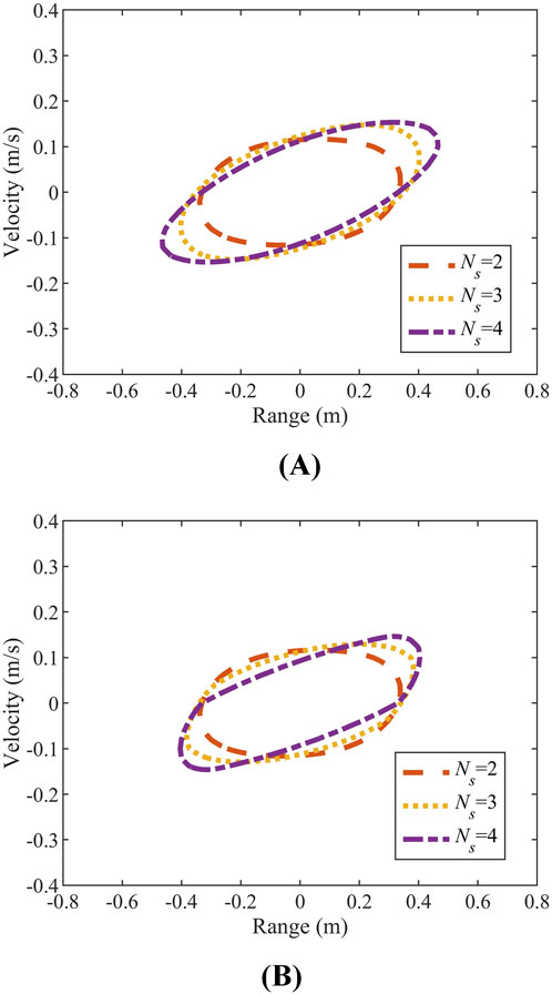
Figure 5. (A) MF resolution cells under three sub-wave number settings. (B) PAMP resolution cells under three sub-wave number settings.

Table 1

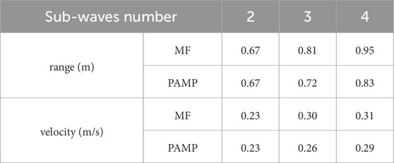
Table 1. Resolution widths comparison.

It can be seen that with the increase of the number of sub-waves, both range and velocity resolution widths increase, which is unfavorable for multi-target resolution. When the number of sub-waves is certain, the resolution widths of PAMP are smaller than PM, which indicates that PAMP can effectively improve the resolution performance. From the perspective of resolution, the number of sub-waves cannot be increased indefinitely, and its selection needs to comprehensively balance the three performance indexes of resolution loss, detection loss and false target probability.

4 Simulation results

Based on the FMC waveform design guidelines [38], a W-LFM waveform is designed, which has a bandwidth $B$ = 1 kHz and a pulse width $T$ = 1 s. Its Time-frequency curve and auto ambiguity function shape are shown in Figure 6. In this section, on the one hand, the two-target simulation signal is processed with high-resolution and the advantage of this paper’s algorithm in the multi-target case is analyzed. On the other hand, based on the ambiguity functions and Q-functions, the advantages of this paper’s algorithm in high-resolution and anti-reverberation performance are compared and analyzed.

Figure 6

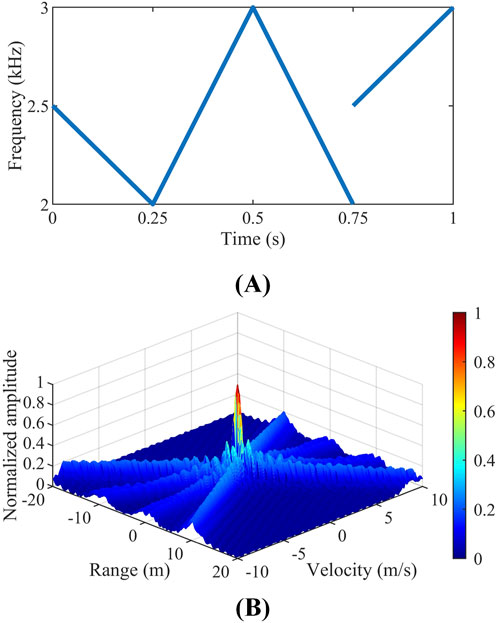
Figure 6. (A) Time-frequency curve of simulation waveform. (B) Auto ambiguity function shape of simulation waveform.

4.1 Ambiguity function shapes of two-target signal

Consider two targets at ranges of 0 m and 10 m, intensities of 0 dB and −3 dB, and velocities of 0 m/s and 5 m/s, respectively. Simulate two W-LFM echo signals formed by the above two targets, one of which is noise-free for the ideal condition, and the other contains Gaussian white noise with SNR = −10 dB for the noise condition. The two signals are processed by four methods, MF, PP, PM and PAMP. Figure 7 shows the ambiguity function shapes of the noise-free signal and Figure 8 shows the ambiguity function shapes of the noise-limited signal.

Figure 7

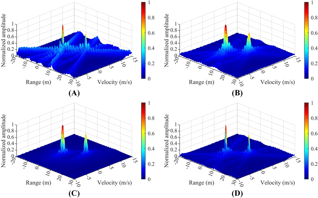
Figure 7. (A) Ambiguity function shapes of noise-free signal for MF. (B) Ambiguity function shapes of noise-free signal for PP. (C) Ambiguity function shapes of noise-free signal for PM. (D) Ambiguity function shapes of noise-free signal for PAMP.

Figure 8

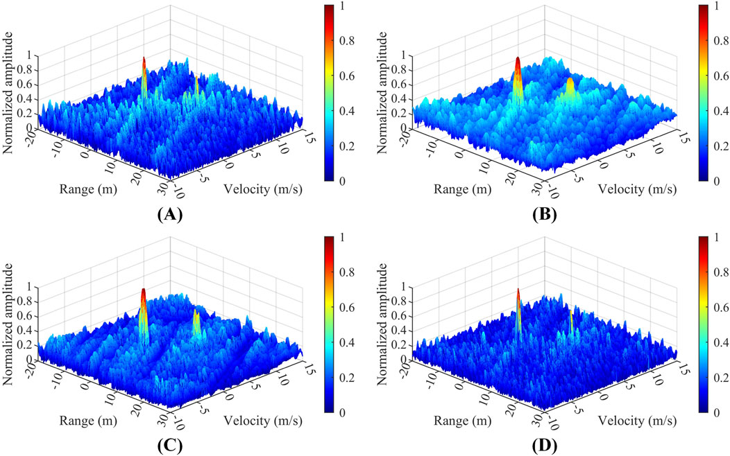
Figure 8. (A) Ambiguity function shapes of noise-limited signal for MF. (B) Ambiguity function shapes of noise-limited signal for PP. (C) Ambiguity function shapes of noise-limited signal for PM. (D) Ambiguity function shapes of noise-limited signal for PAMP.

In Figure 7A, the ridges of the two targets cross each other and form several interference main lobes, which are lower in amplitude than the two real main lobes but have similar structural features to them, which is not conducive to autonomous target identification. Although the backgrounds in Figures 7B–D are relatively flat, the widths of the main lobes of the targets in Figure 7B and C are significantly larger than that in Figure 7D, which indicates that the resolution of PAMP is better than that of PP and PM.

In Figure 8, the overall brightness of the four images increases compared to Figure 7, where Figure 8B has the highest brightness and Figure 8D has the lowest brightness, which means that PP has the largest ambiguity function volume and PAMP has the smallest ambiguity function volume. The ambiguity function volume represents the output reverberation energy of this waveform in the reverberation scenario, and theoretically the smaller the volume the better the anti-reverberation. When there are a large number of densely distributed scattering elements, the high-resolution processing with low background and narrow main lobe can effectively reduce the accumulation of energy and improve the anti-reverberation capability.

4.2 Performance comparison

Consider the theoretical resolution width in auto ambiguity function shape of the FM waveform at −3 dB height. The frequency resolution width is as Equation 15.

$∆\mathit{f}=\frac{\mathbf{1}}{\mathit{T}}={\mathit{f}}_{\mathit{c}}\frac{\mathbf{2}∆\mathit{v}}{\mathbf{c}}(15)$

Pulse width $T$ = 1 s, center frequency $f_c$ = 2.5 kHz, and velocity resolution width $∆v$ = 0.3 m/s. Time resolution width is as Equation 16.

$∆\mathit{t}=\frac{\mathbf{1}}{\mathit{B}}=\frac{\mathbf{2}∆\mathit{d}}{\mathbf{c}}(16)$

Bandwidth $B$ = 1 kHz, sound velocity $\mathrm{c}$ = 1,500 m/s, and range resolution width $∆d$ = 0.75 m.

Figure 9A shows the cross-section in auto ambiguity function shapes of the W-LFM waveform at −3 dB height, i.e., the resolution cell of the signal. Unlike FM, the resolution width of the high-resolution waveform is based on the boundary value of the resolution cell, so it is larger than the theoretical width. The comparison results of the four methods are shown in Table 2.

Figure 9

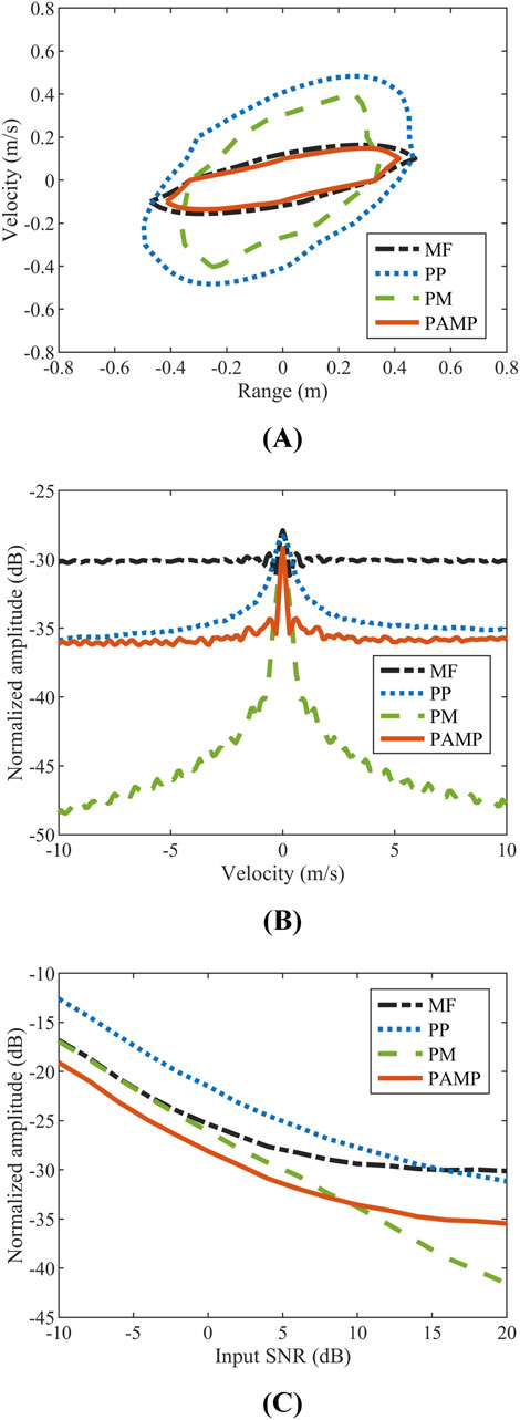
Figure 9. (A) Comparison of range-velocity resolution. (B) Comparison of Q-function. (C) Comparison of SNR-Q curve.

Range resolution width: PM < PAMP < MF < PP, velocity resolution width: PAMP < MF < PM < PP, resolution cell area: PAMP < MF < PM < PP., Compared with MF, the range and velocity resolution widths of PAMP, are reduced by 13% and 10%, respectively. Considering both the width and area of the resolution cell, the W-LFM, waveform processed by PAMP, have the optimal high-resolution performance.

Table 2

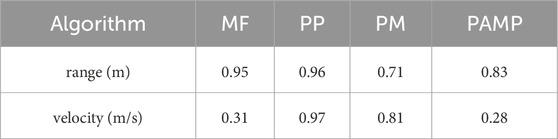
Table 2. Simulated resolution width.

Figure 9B shows the Q-function curves of the W-LFM waveform. The overall height of the Q-function: PP < PAMP < PM < MF. In order to characterize the Q-function curves of the high-resolution algorithms in a low SNR scenario, we examine the Q variation curve about SNR with 5 m/s as an example, and the results are shown in Figure 9C. As the SNR decreases, the Q of all algorithms show an increasing trend. The Q of PM is 16 dB lower than that of MF without noise while SNR <10 dB is higher than that of PAMP, and SNR <−5 dB is close to that of MF. The Q of PP is 5 dB lower than that of MF without noise while SNR <16 dB is higher than that of MF. In contrast, PAMP has a more stable Q variation, with a 6 dB reduction compared to MF in the noiseless case and a 2.5 dB reduction at SNR <−5 dB.

4.3 Summary

Consider a typical case when the detection probability of MF is 0.5, then SNR = −24 dB. The detection probabilities of PP, PM, and PAMP are 0.23, 0.15, and 0.45, and the Qs are −12.6 dB, −16.8 dB and −19.3 dB, respectively.

Although the conventional MF is the receiver with the highest SNR gain, the intersecting ridges in the ambiguity function shape are easy to form interfering bright spots, which are not favorable for target discrimination. The two-target simulation results show that PAMP has strong ridge suppression and target discrimination ability. The resolution performance of PP and PM is lower than that of MF and PAMP, and both of their anti-reverberation advantages are dependent on high SNR of signal, which is not suitable for underwater target detection. However, the PAMP’s anti-reverberation performance is stable in low SNR scenario, where it reduces reverberation by more than 2.5 dB compared to MF, while the detection performance remains close to that of MF.

5 Experiment verification

To verify the practical performance of the FMC signal and the PAMP algorithm, we conducted an active sonar signal test in April 2023 on the lake. The average depth of the experimental area is about 15 meters, and the Signal-to-Interference Ratio (SIR) of the echo is low due to the shallow water. In order to improve the saliency of the target, we set up a detection platform and a simulated target at a relative distance of about 350 m. The detection platform consists of a transducer with a maximum transmitting power of 5 kw and a 12-element standard hydrophone array for transmitting active pulses and receiving signals, respectively. The hydrophones are arranged horizontally and linearly with a spacing of 0.3 m. The simulated target consists of a transducer with a maximum transmitting power of 500 w, which emits Doppler-modulated pulses to simulate a moving target. The deployment depth of the above equipment is 5 m. The experiment situation is shown in Figure 10.

Figure 10

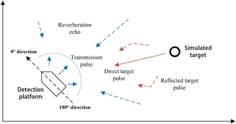
Figure 10. Experiment situation.

The transmit pulses for the test are LFM and W-LFM signals with a pulse width of 1 s and a frequency of 2–3 kHz. The active transducer transmits the pulse at moment 0 of the current detection period, and the target transducer transmits a Doppler-modulated pulse at moment 1.7 s of the current detection period, simulating a moving target with a radial velocity of 1.5 m/s. The signal is received by the hydrophone array throughout the detection period.

5.1 Display image

The received signal is processed with conventional beamforming and matched filtering to obtain a direction-range map for the active sonar. Figure 11 shows the direction-range map of the LFM signal and three main targets labeled in the figure. Target 1 has the shortest range and highest brightness and is considered a direct wave target. Targets 2 and 3 are reflected wave signals, with target 2 being the least bright. There is a bright band near the 90° direction in the figure and a reverberant area in the region within 1.3 km.

Figure 11

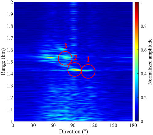
Figure 11. Conventional processing result of LFM signal.

W-LFM is a range-velocity two-dimensional resolution waveform, and the conventional processing cannot realize the detection of moving targets. In order to show the high-resolution processing effect, we calculate the AFs of the beam signals obtained by conventional beamforming, and obtain the direction-velocity-range map. Figure 12 shows the schematic diagram of the direction-velocity-range display.

Figure 12

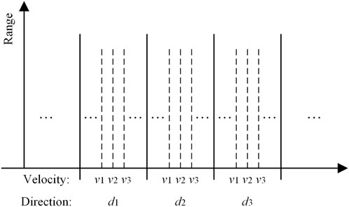
Figure 12. The schematic diagram of direction-velocity-range display.

Figure 13 shows comparatively the direction-velocity-range images of the W-LFM signal, and Figures 13A–D are the processing results of MF, PP, PM, and PMAP, respectively. The four images are normalized by the intensity of their respective direct targets, and they are labeled for the three targets in Figure 11. The parameters (direction/degree, velocity/m/s, range/km) of the three simulated targets are (108, 1.5, 1.44), (92, 1.5, 1.46), and (78, 1.5, 1.56), respectively. Comparing the 4 images, it shows that PAMP has the best overall performance in the following 3 points.

a. Compared to Figure 13D, the reverberant areas of Figures 13A–C are brighter, indicating that the output reverberation of PAMP is the lowest.

b. Compared to Figures 13A, D, the area of the target bright spot is significantly larger in Figures 13B, C, and the center of the bright spot of target 2 is not obvious, indicating that PP and PM have a greater loss of detection performance for weak target. They increase the saliency of strong target but decrease the resolution accuracy.

c. Compared to Figure 13A, the saliency of the target bright spot in Figure 13D is higher due to the elimination effect of PAMP on the ridges, which facilitates target extraction and identification.

Figure 13

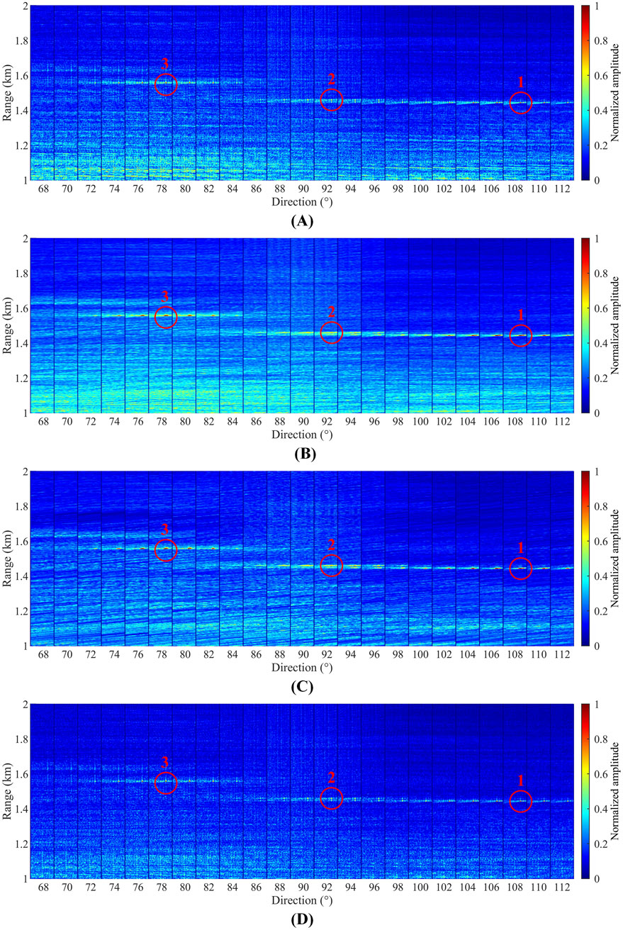
Figure 13. (A) Direction-velocity-range images for MF. (B) Direction-velocity-range images for PP. (C) Direction-velocity-range images for PM. (D) Direction-velocity-range images for PAMP.

5.2 Performance comparison

Figure 14A compares the range-velocity resolution cells of the W-LFM direct wave in the ambiguity function at the height of −3 dB with the 108-degree-direction beam as an example, and the resolution widths are shown in Table 3. The resolution widths of PP and PM are close to each other, while the range resolution width is almost the same and the velocity resolution width is increased by about 2.2 times compared with MF. Meanwhile, compared with MF, the range resolution width of PAMP decreases by about 17% and the velocity resolution width decreases by 10%. The comparison shows that PAMP has the best range-velocity 2-dimensional resolution performance.

Figure 14

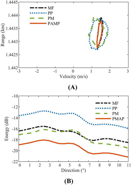
Figure 14. (A) Comparison of range-velocity resolution. (B) Comparison of ambiguity function energy.

Table 3

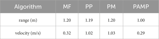
Table 3. Experimental resolution width.

The dual integral of the square of the ambiguity function along range and velocity represents the total energy of the beam, which reflects the output reverberation of a beam. The energy of the beam is expressed as

${\mathit{E}}_{\mathbf{\text{AF}}}={\int }_{{\mathit{v}}_{\mathbf{1}}}^{{\mathit{v}}_{\mathbf{2}}}{\int }_{{\mathit{r}}_{\mathbf{1}}}^{{\mathit{r}}_{\mathbf{2}}}{\left|\mathit{A}\left(\mathit{r},\mathit{v}\right)\right|}^{\mathbf{2}}\mathit{d}\mathit{r}\mathit{d}\mathit{v}$

Figure 14B shows the beam energy curves of the W-LFM signal, where $v_1$ = $-v_2$ = −3 m/s, $r_1$ = 1 km, and $r_2$ = 2 km. Compared to the output reverberation of MF, the average elevation of PP is about 3.1 dB and the average reduction of PM is about 0.5 dB, indicating that neither of the two methods can effectively reduce the output reverberation in the experimental situation. Meanwhile, the output reverberation of PAMP is reduced by about 3.5 dB on average compared to MF, proving the anti-reverberation advantage of PAMP. The above conclusion is consistent with the simulation results in Section 4.2.

6 Discussion

In this paper, we propose an improved high-resolution processing algorithm PAMP for FMC signals based on PP and PM, and verify that PAMP has the performance advantages of little detection loss, high range-velocity resolution, and low reverberation through numerical simulation and lake experiment. In summary, PAMP is suitable for high-resolution processing of hydroacoustic multi-target detection in low SNR background.

In our further work, in addition to continuing the research on high-resolution algorithms, we will conduct target detection experiments of active sonar in more complex acoustic fields. Moreover, we will design comparison experiment with conventional thumbtack signals to further explore the feasibility of FMC signals and high-resolution processing.

Data availability statement

The datasets presented in this article are not readily available because The datasets presented in this article cannot be publicly shared due to privacy restrictions. Requests to access the datasets should be directed to Yaojun Jia, amlheWFvanVuMTEyOUAxNjMuY29t.

Author contributions

YJ: Methodology, Writing–original draft. PW: Supervision, Writing–review and editing. HW: Software, Writing–review and editing. QC: Data curation, Writing–original draft. YH: Software, Writing–original draft.

Funding

The author(s) declare no financial support was received for the research, authorship, and/or publication of this article.

Conflict of interest

The authors declare that the research was conducted in the absence of any commercial or financial relationships that could be construed as a potential conflict of interest.

Generative AI statement

The author(s) declare that no Generative AI was used in the creation of this manuscript.

Publisher’s note

All claims expressed in this article are solely those of the authors and do not necessarily represent those of their affiliated organizations, or those of the publisher, the editors and the reviewers. Any product that may be evaluated in this article, or claim that may be made by its manufacturer, is not guaranteed or endorsed by the publisher.

References

1. Robey FC, Fuhrmann DR, Kelly EJ, Nitzberg R. A CFAR adaptive matched-filter detector. IEEE Trans Aerosp Electron Syst (1992) 28:208–16. doi:10.1109/7.135446

CrossRef Full Text | Google Scholar

2. Chen VC. Radar ambiguity function, time-varying matched-filter, and optimum wavelet correlator. Opt Eng (1994) 33:2212–7. doi:10.1117/12.172252

CrossRef Full Text | Google Scholar

3. Lu X, Tian J, Zhang R, Wang H, Qiu Y. A novel power-combination method using a time-reversal pulse-compression technique. Chin Phys. B (2023) 32:084101. doi:10.1088/1674-1056/acaa2a

CrossRef Full Text | Google Scholar

4. Balleri A, Farina A. Ambiguity function and accuracy of the hyperbolic chirp: comparison with the linear chirp. IET Radar Sonar Navig (2017) 11:142–53. doi:10.1049/iet-rsn.2016.0100

CrossRef Full Text | Google Scholar

5. Liu M, Wang C, Gong J, Tan M, Bao L, Zhou C. Ambiguity function analysis and optimization of coherent FDA radar. IEEE Geosci Remote Sens Lett (2024) 21:1–5. doi:10.1109/LGRS.2024.3406435

CrossRef Full Text | Google Scholar

6. Zhang X, Yang P, Cao D. Synthetic aperture image enhancement with near-coinciding Nonuniform sampling case. Comput Electr Eng (2024) 120:109818. doi:10.1016/j.compeleceng.2024.109818

CrossRef Full Text | Google Scholar

7. Song X, Willett P, Zhou S. Range bias modeling for hyperbolic-frequency-modulated waveforms in target tracking. IEEE J Oceanic Eng (2012) 37:670–9. doi:10.1109/JOE.2012.2206682

CrossRef Full Text | Google Scholar

8. Murray JJ. On the Doppler bias of hyperbolic frequency modulation matched filter time of arrival estimates. IEEE J Oceanic Eng (2019) 44:446–50. doi:10.1109/JOE.2018.2819779

CrossRef Full Text | Google Scholar

9. Wei R, Ma X, Zhao S, Yan S. Doppler estimation based on dual-HFM signal and speed spectrum scanning. IEEE Signal Process Lett (2020) 27:1740–4. doi:10.1109/LSP.2020.3020222

CrossRef Full Text | Google Scholar

10. Doisy Y, Deruaz L, Van Ijsselmuide SP, Beerens SP, Been R. Reverberation suppression using wideband Doppler-sensitive pulses. IEEE J Oceanic Eng (2008) 33:419–33. doi:10.1109/JOE.2008.2002582

CrossRef Full Text | Google Scholar

11. Lee S, Lim J. Reverberation suppression using non-negative matrix factorization to detect low-Doppler target with continuous wave active sonar. EURASIP J Adv Signal Process (2019) 11:11–8. doi:10.1186/s13634-019-0608-6

CrossRef Full Text | Google Scholar

12. Gao B, Li G, Pang J. Velocity extraction of nonlinear internal waves by reverberation detecting in shallow water waveguide. Front Mar Sci (2024) 11:1410399. doi:10.3389/fmars.2024.1410399

CrossRef Full Text | Google Scholar

13. Henyey FS, Tang D. Reverberation clutter induced by nonlinear internal waves in shallow water. J Acoust Soc Am (2013) 134:EL289–93. doi:10.1121/1.4818937

PubMed Abstract | CrossRef Full Text | Google Scholar

14. Hu N, Rao X, Zhao J, Wu S, Wang M, Wang Y, et al. A shallow seafloor reverberation simulation method based on generative adversarial networks. Appl Sci.-Basel (2023) 13:595. doi:10.3390/app13010595

CrossRef Full Text | Google Scholar

15. Cui X, Chi C, Li S, Li Z, Li Y, Huang H. Waveform design using coprime frequency-modulated pulse trains for reverberation suppression of active sonar. J Mar Sci Eng (2023) 11:28. doi:10.3390/jmse11010028

CrossRef Full Text | Google Scholar

16. Wang Y, He Y, Wang J, Shi Z. Comb waveform optimisation with low peak-to-average power ratio via alternating projection. IET Radar Sonar Navig (2018) 12:1012–20. doi:10.1049/iet-rsn.2018.0039

CrossRef Full Text | Google Scholar

17. Noemm M, Hoeher PA. CutFM sonar signal design. Appl Acoust (2015) 90:95–110. doi:10.1016/j.apacoust.2014.10.011

CrossRef Full Text | Google Scholar

18. Kundu NK, Mallik RK, McKay MR. Signal design for frequency-phase keying. IEEE Trans Wireless Commun (2020) 19:4067–79. doi:10.1109/TWC.2020.2979718

CrossRef Full Text | Google Scholar

19. Neuberger N, Vehmas R. A costas-based waveform for local range-Doppler sidelobe level reduction. IEEE Signal Process Lett (2021) 28:673–7. doi:10.1109/LSP.2021.3067219

CrossRef Full Text | Google Scholar

20. Hague DA, Buck JR. The generalized sinusoidal frequency-modulated waveform for active sonar. IEEE J Oceanic Eng (2017) 42:1–15. doi:10.1109/JOE.2016.2556500

CrossRef Full Text | Google Scholar

21. Ben G, Zheng X, Wang Y, Zhang X, Zhang N. Chirp signal denoising based on convolution neural network. Circuits Syst Signal Process (2021) 40:5468–82. doi:10.1007/s00034-021-01727-4

CrossRef Full Text | Google Scholar

22. Patton LK, Frost SW, Rigling BD. Efficient design of radar waveforms for optimised detection in coloured noise. IET Radar Sonar Navig (2012) 6:21–9. doi:10.1049/iet-rsn.2011.0071

CrossRef Full Text | Google Scholar

23. Zhang X, Yang P, Wang Y, Shen W, Yang J, Wang J, et al. A novel multireceiver SAS RD processor. IEEE Trans Geosci Remote Sens (2024) 62:4203611–1. doi:10.1109/TGRS.2024.3362886

CrossRef Full Text | Google Scholar

24. Sibul LH, Titlebaum EL. Volume properties for the wideband ambiguity function. IEEE Trans Aerosp Electron Syst (1981) 17:83–7. doi:10.1109/TAES.1981.309039

CrossRef Full Text | Google Scholar

25. Cui G, Yu X, Yang J, Fu Y, Kong L. An overview of waveform optimization methods for cognitive radar. J Radars (2019) 8:537–57. doi:10.12000/JR16084

CrossRef Full Text | Google Scholar

26. Bhatt TD, Rajan EG, Rao PVDS. Design of high-resolution radar waveforms for multi-radar and dense target environments. IET Radar Sonar Navig (2011) 5:716–25. doi:10.1049/iet-rsn.2010.0364

CrossRef Full Text | Google Scholar

27. Xu Y, Xue M, Liu M, Hao C, Zhao L, Wang J, et al. Wideband waveform design and performance analysis for multiple unmanned underwater vehicle cooperative detection sonar. J Electr Inf Technol (2023) 45:3796–804. doi:10.11999/JEIT221265

CrossRef Full Text | Google Scholar

28. Hague DA, Buck JR. An experimental evaluation of the generalized sinusoidal frequency modulated waveform for active sonar systems. J Acoust Soc Am (2019) 145:3741–55. doi:10.1121/1.5113581

PubMed Abstract | CrossRef Full Text | Google Scholar

29. Liu D, Zhao X, Lu Y. Detection performance analysis of sub-band processing continuous active sonar. Appl Acoust (2021) 174:107700. doi:10.1016/j.apacoust.2020.107700

CrossRef Full Text | Google Scholar

30. Zhang X, Tan C, Ying W. An imaging algorithm for multireceiver synthetic aperture sonar. Remote Sens (2019) 11:672. doi:10.3390/rs11060672

CrossRef Full Text | Google Scholar

31. Suga N, Schlegel P. Coding and processing in the auditory systems of FM-signal-producing bats. J Acoust Soc Amer (1973) 54:174–90. doi:10.1121/1.1913561

PubMed Abstract | CrossRef Full Text | Google Scholar

32. Vespe M, Jones G, Baker CJ. Lessons for radar: waveform diversity in echolocating mammals. IEEE Signal Process Mag (2009) 26:65–75. doi:10.1109/MSP.2008.930412

CrossRef Full Text | Google Scholar

33. Lu Y, Wang F, Wu H. Waveform anti-clutter performance analysis of the bio-sonar of a flying bat. J China Acad Electr Inf Technol (2023) 18:755–60. doi:10.3969/j.issn.1673-5692.2023.08.011

CrossRef Full Text | Google Scholar

34. Rasool SB, Bell MR. Biologically inspired processing of radar waveforms for enhanced delay-Doppler resolution. IEEE Trans Signal Process (2011) 59:2698–709. doi:10.1109/TSP.2011.2121904

CrossRef Full Text | Google Scholar

35. Zhu J, Song Y, Fan C, Huang X. Nonlinear processing for enhanced delay-Doppler resolution of multiple targets based on an improved radar waveform. Signal Process (2017) 130:355–64. doi:10.1016/j.sigpro.2016.07.025

CrossRef Full Text | Google Scholar

36. Zhu J, Yin T, Guo W, Zhang B, Zhou Z. An underwater target azimuth trajectory enhancement approach in BTR. Appl Acoust (2025) 230:110373. doi:10.1016/j.apacoust.2024.110373

CrossRef Full Text | Google Scholar

37. Lou L, Wang P. A high resolution waveform design based on hyperbolic frequency modulation combination. Ship Electron Eng (2020) 40:154–8. doi:10.3969/j.issn.1672-9730.2020.10.037

CrossRef Full Text | Google Scholar

38. Jia Y, Cai Z, Wang P. Research on combination waveform design based on hyperbolic frequency modulation. J Electr Inf Technol (2023) 45:4352–60. doi:10.11999/JEIT221385

CrossRef Full Text | Google Scholar

39. Liu F, Hu Y, Rao P, Gong C. Modified point target detection algorithm based on Markov random field. Int J Infrared Millimeter Waves (2018) 37:212–8. doi:10.11972/j.issn.1001-9014.2018.02.014

CrossRef Full Text | Google Scholar

40. Zhang X. An efficient method for the simulation of multireceiver SAS raw signal. Multimedia Tools Appl (2023) 83:37351–68. doi:10.1007/s11042-023-16992-5

CrossRef Full Text | Google Scholar

41. Collins T, Atkins P. Doppler-sensitive active sonar pulse designs for reverberation processing. IEE Proc.-Radar Sonar Navig. (1998) 145:347–53. doi:10.1049/ip-rsn:19982434

CrossRef Full Text | Google Scholar