Regional simulations of equatorial spread F driven with, and an analysis of, WAM-IPE electric fields

A three-dimensional, regional simulation is used to investigate ionospheric plasma density irregularities associated with Equatorial Spread F. This simulation is first driven with background electric fields derived from ISR observations. Next, the simulation is driven with electric fields taken from the WAM-IPE global model. The discrepancies between the two electric fields, particularly in the evening prereversal enhancement, produce disagreeing simulation results. The WAM-IPE electric fields are then studied through a simple sensitivity analysis of a field-line integrated electrodynamics model similar to the one used in WAM-IPE. This analysis suggests there is no simple tuning of ion composition or neutral winds that accurately reproduce ISR-observed electric fields on a day-to-day basis. Additionally, the persistency of the prereversal enhancement structure over time is studied and compared to measurements from the ICON satellite. These results suggest that WAM-IPE electric fields generally have a shorter and more variable correlation time than those measured by ICON.

1 Introduction

Equatorial Spread F (ESF) is a broad term that refers to a wide range of phenomena observed in the equatorial F-region ionosphere associated with post-sunset instabilities. Its name is derived from its effect of “spreading” ionograms that was first reported by [1]. The associated plasma density irregularities are primarily attributed to collisional interchange instabilities [2–4] or inertial interchange instabilities [3]. Collisional shear instability has been proposed as a preconditioner for ESF activity [5]. The resulting irregularities can cause the scintillation of radio waves traveling through the region. This can compromise critical systems such as communication, navigation, and imaging systems [6, 7]. Avoiding these hazards requires an accurate forecast of ESF events that perform better than climatological estimates. For the purposes of this study, an accurate forecast is one that predicts the presence or absence of robust irregularities on a night-to-night basis and can be validated with radar or satellite observations.

The earliest attempts at forecasting ESF involved analyzing linear growth rates estimated from field-line integrated quantities [8, 9]. These approaches predicted the climatological patterns of ESF occurrences. However, they were unable to produce accurate night-to-night behavior. Additionally, linear growth rate methods failed to explain the observation of topside irregularities. Other forecast attempts have involved numerical simulations of ESF and its associated irregularities. One of the first simulations that showed topside irregularities was presented by [10]. They showed the nonlinear evolution of interchange instabilities into equatorial plasma bubbles (EPBs) that reached the topside ionosphere. Despite these EPBs penetrating the topside ionosphere, they took significantly longer to develop than bubbles observed in nature. Current work aims at pairing observational data with direct numerical simulations. The observational data can be provided by incoherent radar scatter (ISR) observations taken at Jicamarca Radio Observatory [11] or satellite data such as that from the ICON satellite [12, 13].

One important factor in identifying favorable conditions for ESF and predicting its development is the large-scale zonal electric fields near the day/night terminator. These electric fields produce the vertical $\mathbf{E}\times \mathbf{B}$ plasma drifts that raise and lower the ionosphere. Of particular interest is the evening prereversal enhancement (PRE) that is commonly observed prior to sunset. The strength and timing of the PRE have been closely associated with the occurrence of ESF [14]. Accurately predicting the PRE is crucial for forecasting ESF. Multiple theories of the PRE have been suggested [15–17] and have been shown to produce the PRE in numerical models [18]. A common feature of these theories is a neutral thermospheric wind that generates a dynamo electric field in the equatorial F-region and off-equatorial E-regions. Near the day/night terminator, the steep zonal gradient in conductivity causes this dynamo to produce an enhanced eastward electric field. The lack of a similar but reverse phenomenon in the morning near the dawn terminator is yet to be explained thoroughly. The climatology of the PRE is well captured by the empirical drifts model proposed by [19]. However, the high degree of day-to-day variability remains an open question in equatorial electrodynamics. The regional simulation for ESF that is used in this study has previously been shown to be most sensitive to the strength of the PRE [13] as well as its timing and duration [20].

In this study, observational data are replaced with estimates from a global circulation model (GCM). As in [20], the GCM used is the Whole Atmosphere Model with Ionosphere, Plasmasphere, and Electrodynamics (WAM-IPE) from NOAA. WAM-IPE is run operationally at NOAA Space Weather Prediction Center (SWPC) providing ionospheric and neutral atmosphere state parameter estimates from inputs of solar and geomagnetic activity and lower atmospheric forcing [21]. The model extends the Global Forecast System vertically to approximately 600 km altitude and includes additional upper atmospheric physics. These additional physics involve one-way coupling to an ionosphere-plasmasphere model and a self-consistent electrodynamics solver similar to that used in the NCAR TIE-GCM model [22]. Here, the electric fields produced by this dynamo solver are studied, and their impact on a regional simulation of ESF-related irregularities is analyzed. It is believed that the day-to-day disagreement between WAM-IPE-produced and ISR-observed electric fields prevents accurate reproductions of ESF activity. This conclusion prompts a further analysis of WAM-IPE electric fields and testing whether they can be adjusted in a way that will match ISR observations.

The remainder of this paper is structured as follows. In Section 2, we discuss the regional simulation used to replicate ESF observations. Results from an August/September 2022 campaign are presented and the effects of WAM-IPE electric fields are analyzed. In Section 3, a proxy electrodynamics model is described and used to perform a variety of sensitivity tests on the dynamo electric fields from WAM-IPE. The tests here include adjustments to ionospheric composition and the structure of the thermospheric neutral winds. The effects of these tests are then compared to ISR observations for all nights of the campaign. Next, in Section 4, we compare the temporal evolution of the PRE in WAM-IPE to that observed by the ICON satellite. Correlation times of this structure are discussed and compared to theory. Finally, Section 5 summarizes the results and provides a brief discussion on advancing toward a true forecast of ESF events.

2 Regional simulation

The regional simulation used here is a three-dimensional, multifluid simulation cast in magnetic dipole coordinates [23,24]. It tracks the number densities of four ion species ($H^{+}$, $N{O}^{+}$, $O_2^{+}$, and $O^{+}$) and electrons. Results are validated through comparison with both coherent and incoherent radar observations of irregularities. The simulation was described in detail by [11] and is used here similarly to [20]. For this reason, only a brief description of it is given here.

There are two primary computations performed in the simulation. The first is a linear solver that calculates the electrostatic potential associated with the small-scale electric fields present in irregularities. This means the electric field is broken into two components: a large-scale background electric field ${\mathbf{E}}_0$, and a gradient of a scalar potential defining the small-scale electric fields, $-\nabla \mathrm{\Phi }$. Starting from the inertialess momentum equation and using this split electric field, one can find the following elliptic PDE by enforcing the divergence-free current condition $(\nabla \cdot \mathbf{J}=0)$.

$\nabla \cdot \left(\sigma \cdot \nabla \mathrm{\Phi }\right)=\nabla \cdot \left[\sigma \cdot \left({\mathbf{E}}_0+\mathbf{u}\times \mathbf{B}\right)-{\displaystyle \sum _s}{q}_s{\mathbf{D}}_s\cdot \nabla n_s+\mathrm{\Xi }\cdot \mathbf{g}\right](1)$

where $\sigma$ is the conductivity tensor, $\mathrm{\Phi }$ is the electrostatic potential, ${\mathbf{E}}_0$ is the background electric field, $\mathbf{u}$ is the neutral thermospheric wind vector, $\mathbf{B}$ is the geomagnetic field, $q_s$ is the electric charge of species $s$, ${\mathbf{D}}_s$ is the diffusivity tensor for a species, $n_s$ is the species number density, $\mathbf{\Xi }$ is a tensor containing all the terms describing gravity-driven currents, and $\mathbf{g}$ is the Earth’s gravitational field. Equation 1 is solved using a preconditioned stabilized biconjugate gradient method with Robin boundary conditions on all boundaries.

The second computation is a finite-volume code that updates species according to the continuity equation, given by Equation 2.

$\frac{\partial n_s}{\partial t}+\nabla \cdot \left(n_s{\mathbf{v}}_s\right)=P-L(2)$

where ${\mathbf{v}}_s$ is the drift velocity that is calculated using the inertialess momentum equation, and $P$ and $L$ are production and loss terms. The chemical production and loss rates for charge exchange and dissociative recombination are taken from [25]. A flux assignment scheme based on the total variation diminishing (TVD) condition is used with monotone upwind scaling for conservation laws (MUSCLs). Time advancement is performed with a second-order Runge-Kutta scheme with time steps of 7.5 s for 2 h.

Initialization of the simulation is done with empirical and physics-based models paired with ISR observations. Ion composition is initialized with IRI-2016, and electron density is initialized by tuning SAMI2 to produce electron density profiles that are in agreement with ISR observations. This tuning is done in two ways: adjusting the F10.7 solar flux parameter and adjusting a second parameter that controls the time history of the background electric fields. Both of these parameters are adjusted until there is optimal congruity between SAMI2-produced profiles and those observed through ISR, as shown in each panel B in Figure 1. This tuning is typically minimal and does not have a large impact on simulation results. Since SAMI2 is a two-dimensional model operating at a single longitude, local time and longitude are considered to be equivalent in order to extrapolate the SAMI2 results to neighboring longitudes. Parameters describing the neutral atmosphere are continuously taken from NRLMSIS 2.0 throughout the simulation.

Figure 1

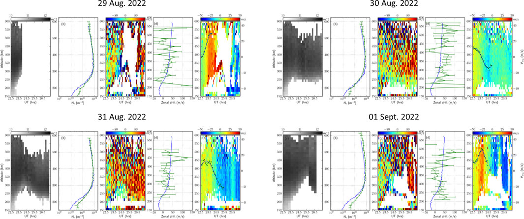
Figure 1. ISR data for all four nights of the 2022 campaign. Shown for each night from left to right is (A) electron number density, (B) an electron number density profile at 2300 UT, (C) zonal plasma drift velocities, (D) a zonal plasma drift velocity profile at 2300 UT, (E) vertical plasma drift velocities. The green curves in panels (B) and (D) represent ISR-measured values, while the blue curves represent model values (SAMI2 and HWM14, respectively). Plotted against the far right axis in all (E) panels are the height-averaged vertical plasma drifts (green scatter points) and the sinusoidal parameterization given by Equation 3 (blue curve).

The driving terms include the background electric fields, ${\mathbf{E}}_0$, and neutral thermospheric winds, ${\mathbf{u}}_0$. These are also derived from empirical models and ISR observations. Additionally in this study, the electric fields can be derived from WAM-IPE estimates. HWM14 prescribes the neutral winds throughout the simulation. These winds can be tuned via a multiplicative factor to produce zonal plasma drifts that agree with ISR observations. No such tuning was necessary for the results shown here. In this study, simulation results are compared where the background electric fields are derived from ISR vertical plasma drift measurements, and taken directly from WAM-IPE. Another source for these electric fields that has been explored is those taken from the ion velocity meter (IVM) aboard the ICON satellite [12, 13].

Multiple ISR experiments have been run at Jicmarca Radio Observatory over the last few years. These ISR experiments provide estimates for multiple state parameters of the ionosphere including plasma number density, electron and ion temperatures, and zonal and vertical plasma drift velocities. Figure 1 shows ISR data for all four nights of a 2022 campaign during the hours surrounding sunset. Blank patches in the ISR data correspond to coherent scatter from 3-m irregularities that interfere with the ISR technique and prevent parameter estimation. These irregularities are closely associated with ESF and serve as an indicator of ESF activity here. It can be seen in Figure 1 that 29 Aug. and 01 Sept. experienced particularly strong ESF events with large depletion plumes penetrating the topside ionosphere.

Plotted in green against the right vertical axis in each (e) panel of Figure 1 are height-averaged vertical plasma drift velocities. These averaged drift speeds are parameterized using a sinusoidal function with four parameters: amplitude, $V_0$, period, $\tau$, UT hour offset, $t_0$, and vertical offset, $c$.

$v\left(t\right)=V_0\sin \left(\frac{2\pi }{\tau }\left(t-t_0\right)\right)+c(3)$

This parameterization describes the zonal background electric fields throughout the 2-hour simulation and adequately captures the strength, timing, and duration of the PRE. It is plotted in blue against the right vertical axis in each (e) panel of Figure 1. The PRE is regularly observed by Jicamarca ISR experiments and it is important to capture for predicting ESF activity.

2.1 Simulation results

Figure 2 shows simulation results for four nights of a 2022 campaign when driven with ISR-derived electric fields. All four nights were during a geomagnetically quiet period. Results are shown 2 hours after initialization, which took place at 2300 UT for the first two nights and 2310 UT for the last two nights. They show ionospheric composition in a zonal-altitudinal slice in the magnetic equatorial plane. Red, green, and blue coloring represents molecular ion, proton, and atomic oxygen ion number density. Strong ESF activity is visible during the first and fourth nights of the campaign in the form of large depletion plumes. These large depletion plumes penetrate well into the topside ionosphere within 2 h of their initialization. This closely resembles the radar observations shown in Figure 1, for all nights of the campaign. These results act as a validation of the regional simulation.

Figure 2

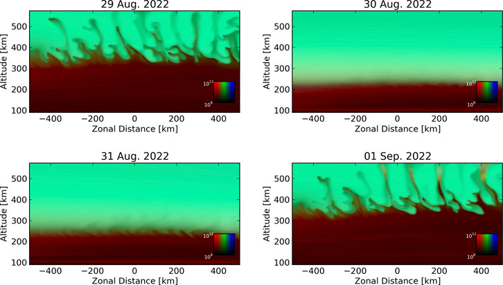
Figure 2. Simulation results for four nights of an Aug. 2022 campaign, when driven with ISR-derived electric fields. Ion number densities are represented with brightness according to the scale in the lower-right-hand corner. Red, green, and blue colors represent molecular ions, protons, and atomic oxygen ions. Ion densities are given in units of ${\text{m}}^{-3}$. Simulation results are shown 2 h after initialization time (see text).

Figure 3 also shows simulation results for the same August/September 2022 campaign with the simulation driven by WAM-IPE background electric fields. Additionally, WAM-IPE provided the initial ion composition and neutral compositions throughout the simulation. The most significant difference between results in Figures 2, 3 is the absence of plumes on the nights of 29 Aug. and 01 Sept. These are examples of missed detections of ESF. ESF activity was observed during both of these nights and replicated in simulations driven with radar data but absent in simulations driven with WAM-IPE estimates. Figure 4 shows the differences between vertical plasma drifts (via zonal background electric fields) in ISR observations (red) and WAM-IPE results (blue) for all four nights of the campaign. It can be seen that the particularly strong PRE observed by ISR on the first and fourth nights is absent in WAM-IPE. This lack of a PRE prevented the rapid growth of irregularities in the simulation. The two nights without ESF activity have significantly weaker PREs and show better agreement between WAM-IPE and ISR.

Figure 3

Figure 3. Same as Figure 2, but with the simulation being driven with WAM-IPE background electric fields.

Figure 4

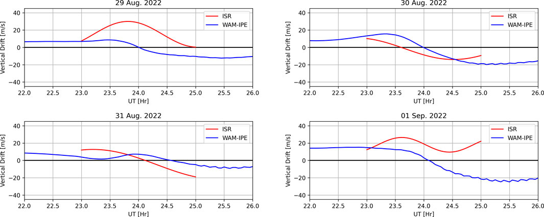
Figure 4. Vertical plasma drift velocities taken from ISR observations (red) and WAM-IPE results (blue) for all nights of the 2022 campaign. WAM-IPE values are taken to be at 300 km altitudes directly overhead Jicamarca.

Another visible difference between the two results is that WAM-IPE exhibits an enhanced molecular ion composition in the valley region compared to that predicted by IRI-2016. This is most noticeable between 100 and 200 km altitudes for all nights in Figure 3. The effects of substituting WAM-IPE compositions into the simulation while being driven with ISR-derived electric fields was studied by [20] along with wind substitutions and electric field substitutions on multiple nights during a Sept. 2021 campaign. Those results indicated that WAM-IPE composition is likely not the source of discrepancy in simulation results. The same conclusion is reached here by noting that the enhanced molecular ion density occurs on all four nights. Missed detections only occur on the nights when WAM-IPE electric fields disagreed with ISR observations. This compositional difference is noted as it is the motivation for studying the effects of enhanced molecular ion densities on the development of electric fields discussed in the following section.

3 Electrodynamics sensitivity analysis

A two-dimensional electrodynamics solver similar to the one used in WAM-IPE was built to serve as a proxy model for WAM-IPE electric fields. The model uses modified apex coordinates [26, 27] and an IGRF magnetic field [28]. In this coordinate system, the two dimensions that are constant along a magnetic field line are the apex longitude, $\varphi$, and the modified apex latitude, $\lambda$. The apex longitude is defined as the centered-dipole longitude of the field line’s apex point. The modified apex latitude is defined to be the latitude that a dipole field line with the same apex altitude, $h_A$, would intersect with a constant reference height $h_R$. Here, a reference height of 90 km is used as that is considered to be the base of the conducting ionosphere.

Magnetospheric sources are neglected, confining the model to magnetic latitudes below $\pm 60°$. These magnetic latitudes are equivalent to apex heights ranging from 90 km to 19,373 km. Assuming equipotential field lines (as done by [29]), the field-line integrated divergence-free current condition results in the following two-dimensional PDE for electrostatic potential, $\mathrm{\Phi }$.

$\begin{array}{ll}\hfill & \frac{\partial }{\partial \varphi }\left(\frac{{\mathrm{\Sigma }}_{\varphi \varphi }}{\cos \lambda }\frac{\partial \mathrm{\Phi }}{\partial \varphi }+{\mathrm{\Sigma }}_{\varphi \lambda }\frac{\partial \mathrm{\Phi }}{\partial |\lambda |}\right)+\frac{\partial }{\partial |\lambda |}\left({\mathrm{\Sigma }}_{\lambda \varphi }\frac{\partial \mathrm{\Phi }}{\partial \varphi }+{\mathrm{\Sigma }}_{\lambda \lambda }\cos \lambda \frac{\partial \mathrm{\Phi }}{\partial |\lambda |}\right)\hfill \\ \hfill & =\left(R_E+h_R\right)\left(\frac{\partial K_{\varphi }^D}{\partial \varphi }+\frac{\partial }{\partial |\lambda |}\left[K_{\lambda }^D\cos \lambda \right]\right)\hfill \end{array}(4)$

where $R_E$ is the mean radius of the Earth (6,371.2 km), ${\mathrm{\Sigma }}_{\varphi \varphi }$ and ${\mathrm{\Sigma }}_{\lambda \lambda }$ act in a similar manner as integrated Pedersen conductivities, ${\mathrm{\Sigma }}_{\varphi \lambda }$ and ${\mathrm{\Sigma }}_{\lambda \varphi }$ act similar to integrated Hall conductivities, and $K_{\varphi }^D$ and $K_{\lambda }^D$ are integrated “wind-driven” current densities that act as source terms for the ionospheric dynamo. All quantities in Equation 4 are constant along a magnetic field line and can be mapped down to a desired height along that field line. A more detailed derivation of Equation 4, along with definitions of integrated quantities, is given in Supplementary Appendix A and [26].

In reality, there is a small potential drop along magnetic field lines suggesting that the electrostatic potential is truly a three-dimensional structure. However, resolving this 3D global structure at a high enough resolution to capture the PRE would be computationally intensive. This is not a concern here as the purpose of this model is to serve as a proxy to the WAM-IPE electrodynamics model which makes the same equipotential field line assumption. Additionally, gravity and pressure-driven currents are also neglected here, although their effects were studied by [30].

The resolution of the model is 4.5$°$ in the $\varphi$ direction and 1.0$°$ in the $\lambda$ direction. While the grid is uniform in the modified apex latitude dimension, this does not equate to uniform spacing in the apex altitude of field lines. WAM-IPE densities and neutral winds are interpolated to irregularly spaced points along each magnetic field line and then integrated in the manner given in Supplementary Appendix A. The spacing of field line points is determined by the altitudinal distance between neighboring points with 1 km spacing below 150 km, 5 km spacing between 150 and 2000 km, and 100 km spacing above 2000 km. This allows for a better representation of E-region dynamics that occur near the base of the field lines and drive the Sq current system. In solving Equation 4, periodic boundary conditions are used in the $\varphi$ direction. Due to the lack of magnetospheric current sources, the high latitude/altitude boundary condition is $\mathrm{\Phi }=0$. The current in the $\lambda$ direction is restricted to zero at the low latitude/altitude boundary (i.e., $K_{\lambda }=0$).

3.1 Model results

Shown in Figure 5 are the results of the proxy model taken at 2300 UT on 29 Aug. 2022. At this time the day/night terminator is located approximately 7$°$ East of Jicamarca, which is indicated by the vertical orange line in each panel. The values shown in Figure 5 are (a) the electrostatic potential for all modified apex latitudes, (b) upward plasma drift velocities between 100 and 600 km apex altitudes, and (c) upward plasma drift velocities at 300 km altitude compared to WAM-IPE results. The contours of electrostatic potential in Figure 5A act as flowlines for plasma drifts, with clockwise flow around local maxima and counter-clockwise flow around local minima. The enhanced upward velocity that’s indicative of the PRE can be seen a few degrees to the East of Jicamarca in each panel. Additionally, Figure 5C validates the proxy model as a reasonable replication of WAM-IPE electric fields.

Figure 5

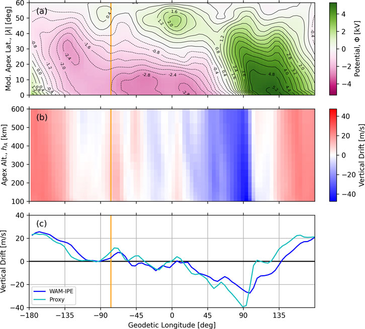
Figure 5. Results from the proxy electrodynamics model for all longitudes at 2300 UT of 29 Aug. 2022. (A) Electrostatic potential and contours, for all modified apex latitudes. (B) Vertical plasma drifts (positive upwards) in the magnetic equatorial plane for apex heights ranging from 100–600 km. The PRE is most prevalent at these altitudes. (C) Upward plasma drifts at 300 km altitude from WAM-IPE are shown in the dark blue while proxy model solutions are shown in the light blue curve. The orange line indicates the location of Jicamarca Radio Observatory (76.87$°$E longitude).

To compare directly to ISR measurements, the proxy model is solved at 12-minute increments from 2200 UT to 0200 UT. The plasma drift velocities 300 km overhead Jicmarca are recorded and plotted alongside WAM-IPE values. Figure 6 shows time series of zonal and vertical plasma drift velocities from all nights of the 2022 campaign. Note that the proxy model solutions (solid cyan curves) agree with WAM-IPE estimates (solid dark blue curves) within reason. This provides further validation for the model to act as a proxy for WAM-IPE electrodynamics. The first and fourth nights exhibit significant disagreement between the PRE in WAM-IPE and ISR observations (solid red curves), while the second and third nights show similarly small PRE patterns. The dashed lines plotted in Figure 6 show results from the proxy model due to the various sensitivity tests discussed below.

Figure 6

Figure 6. Time series of proxy model plasma drifts taken 300 km overhead Jicamarca, compared to WAM-IPE results and ISR observations for each night of the 2022 campaign. Shown for each night are (A) zonal drift velocities and (B) vertical drift velocities. Additionally, results from each sensitivity test are plotted to visualize their impacts on the dynamo electric fields.

The first sensitivity tested relates to ionospheric composition and is motivated by the observation of enhanced molecular ion densities in WAM-IPE mentioned in Section 2.1. In this test, the proxy model was tested with only 10% of the original molecular ions given by WAM-IPE. Results from this test are plotted in dashed orange lines in Figure 6. Since the decrease of ions in the ionosphere diminishes the conductivity, larger electric fields (therefore larger plasma drift magnitudes) are required to maintain the same current flow. Despite the larger fields, there are minimal effects on the structuring of the PRE, and vertical drifts do not appear to match ISR observations any better than when the full WAM-IPE composition is used. This acts as further validation of the claim that enhanced molecular ion densities are not the source of inaccurate simulation results.

The next two tests involve using HWM14 winds to drive the dynamo electric fields rather than thermospheric winds provided by WAM-IPE. The first of these tests is a direct substitution of HWM14 winds and is shown in dashed dark green lines, while a second test uses HWM14 winds delayed by 1 hour and is shown in dashed light green lines. The 1-h delay is motivated by results in [13], where this offset produced optimal agreement with ICON satellite wind measurements. Both tests have similar impacts on the time series of horizontal and vertical drifts. It can be seen that these had the most significant impact on the proxy model vertical drifts and improved the agreement with ISR observations on 29 Aug. 2022. However, each of these tests produced a similar PRE on all four nights including the two nights when a weak PRE was observed. This is not surprising as HWM14 is an empirical model that does not capture rapid day-to-day variations.

The final two tests are motivated by results from [31] where it was found that the PRE structure was sensitive to the zonal winds located at magnetic latitudes near the Equatorial Ionization Anamoly (EIA), rather than only those near the day/night terminator. Their results suggested that eliminating the zonal winds near the EIA, diminished the magnitude of the PRE. To test this, the proxy model was first run with no zonal winds for all longitudes where $20\le |\lambda |\le 40$ (shown in dashed pink lines) and then with double the zonal winds in the same region (shown in dashed purple lines). The results here agree with those in [31], with a generally decreased drift magnitude with no EIA winds, and an increased drift magnitude with double EIA winds. However, neither of these tests produced a PRE comparable to that observed by ISR, on either night.

As can be seen in each panel (a) of Figure 6, none of these sensitivity tests significantly impacted the evolution of zonal drift velocities. The regional simulation described above does not appear to be highly sensitive to zonal drifts. However, it is highly sensitive to vertical drifts. Both of these observations highlight the importance of predicting the vertical plasma drifts and the structure of the PRE in forecasting ESF.

4 PRE persistance

The final analysis of WAM-IPE electric fields performed here is on the persistence of the PRE in both magnitude and timing. The empirical model developed by [19] and used in many ionospheric models predicts a global structure of vertical plasma drifts that is predominantly dependent on LT. This means that the PRE can be expected to remain roughly constant in magnitude and position relative to the day/night terminator. Therefore, if the PRE is sampled at the same LT at two different UTs, there should be a strong correlation between the two curves. This is not always observed in WAM-IPE estimates of the vertical plasma drifts.

Figure 7 shows the evolution of WAM-IPE vertical drifts in UT for a span of LT surrounding the day/night terminator. Drifts are shown at 300 km altitude for all nights of the 2022 campaign are shown in 12-minute increments between 2300 UT and 0100 UT. The LT for each panel is constant with the terminator (1830 LT) in the center of the horizontal axis. The UT increases moving down a column, so each subsequent panel moves to the west in longitude. It can be seen that the PRE structure does not remain constant across the 2 hours of samples, and can change rapidly across 36 min, or less. In general, both the PRE peak and the reversal time drift to the west as the night progresses. One significant observation is the disappearance and reappearance of the PRE on 29 Aug. (first column). The PRE is absent at 2348 UT but is weakly present 12 min before and after. It is expected that the PRE would be present, and maintain its magnitude and position, throughout the entire night rather than appear and disappear rapidly.

Figure 7

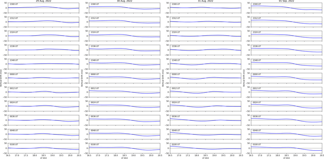
Figure 7. WAM-IPE vertical plasma drifts at 300 km altitude as a function of Local Time surrounding the day/night terminator (1830 LT) at 12-minute increments spanning 2 h in UT. All four nights of the 2022 campaign are shown in respective columns. Each subsequent row is 12 min later in UT than the one above it. To follow the terminator properly, each subsequent panel is therefore observing longitudes that are 3$°$ to the west of the previous panel.

To study this evolution of the PRE, in-situ data provided by the IVM device aboard the ICON satellite is used for comparison. Ion velocities from ICON are recorded as the satellite passes the magnetic equator near sunset. These measurements were used as a driver of the regional simulation by [12] and [13]. Results presented in those studies highlighted the importance of the PRE in driving the regional simulation. Normalized autocorrelation functions of vertical plasma drift measurements were calculated from consecutive orbits separated by 104 min (the orbital period of ICON). These functions are shown in Figure 8, with red curves representing data from August 2022, and blue curves representing data from October 2022. Bright-colored curves indicate nights when ESF was observed, while pastel-colored curves indicate no ESF activity. The lag time on the horizontal axis represents the lag time relative to when ICON crosses a constant LT sector. Due to the satellite’s motion, both temporal and spatial variations are implicitly represented in these datasets. This is not the same as recording the spatial structure of the PRE at a constant LT as is done in Figure 7. However, it is an in-situ measurement that can be used as a baseline for the persistence of the PRE.

Figure 8

Figure 8. Autocorrelation functions of vertical plasma drifts measured by the IVM on the ICON satellite. All orbits are plotted together. Correlations are taken between plasma drifts measured in sequential passes of the ICON satellite through the magnetic equator near sunset. Sequential passes are separated in UT by 104 min. Red colors show August 2022 data and blue colors show October 2022 data. Bright-colored lines indicate nights when ESF irregularities were observed by the satellite, while pastel-colored lines indicate nights when ESF irregularities were not observed. The black dashed line indicates a correlation coefficient of $1-e^{-1}$.

It can be seen in Figure 8 that the PRE is well correlated across at least 104 min. Here, the correlation time, $t_{\mathit{corr}}$ is defined as the maximum time between measurements with a correlation coefficient that has decreased by a factor less than or equal to $1/e$. Since relatively few autocorrelation functions in Figure 8 have a maximum correlation coefficient less than $1-e^{-1}$ (dashed black line), it is concluded that ICON data suggests a correlation time longer than 104 min. Additionally, the location of the PRE remains relatively constant, as indicated by the small lag times of the peak correlation coefficient. Nights in which ESF was observed exhibit a particularly strong correlation relative to nights without ESF. Based on these results, it can be concluded that the PRE has a correlation time of at least 104 min. This large $t_{\mathit{corr}}$ is in agreement with the empirical model suggested by [19].

Similar, but not equivalent, normalized autocorrelations are taken with WAM-IPE estimates of vertical plasma drifts throughout 2021 and 2022 campaigns and are shown in Figures 9, 10 (WAM-IPE data for the 2021 campaign were analyzed by [20]). The estimates of vertical drifts are recorded at 590 km altitude (the orbital altitude of ICON satellite) and across a 60$°$ wide longitude sector centered around the day/night terminator. Contradictory to the ICON data shown in Figure 8, this solely compares the spatial structure of the PRE. This longitude sector corresponds to $\pm$2 h in LT around the terminator. Autocorrelation functions are calculated by correlating these sectored vertical drifts at two different UTs. Autocorrelation functions with the same UT lag time are then averaged. For example, a 3-minute UT lag time correlation is calculated between 2300 UT and 2303 UT, between 2303 and 2306 UT, between 2306 UT and 2309 UT, and so on before being averaged. The UT lag times are then increased by 3 min until a UT lag time of 120 min is reached or $t_{\mathit{corr}}$ is reached. Correlation times are printed in the upper-left-hand corner of each panel in Figures 9, 10. The horizontal axis is the LT shift (equivalent to a longitudinal shift) of the two longitudinal sectors relative to one another. A positive LT shift corresponds to an Eastward shift. The color of each line plotted is representative of the UT lag time between longitudinal sectors that are being correlated. This essentially separates the spatial and temporal structure of the plasma drifts, which were combined for the ICON data.

Figure 9

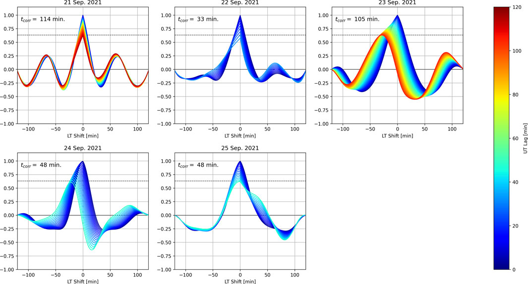
Figure 9. Autocorrelation functions of WAM-IPE vertical plasma drifts from 2021 campaign. The horizontal axis is the LT shift (in minutes) of the PRE structure with negative values corresponding to a Westward shift. Multiple autocorrelation functions are plotted on each axis with the color of each line representing the UT lag between the curves being correlated. Details for how these functions are calculated are given in the text. Autocorrelation functions are plotted for increasing lag times until the correlation coefficient decreases by a factor of $1/e$ (dashed black line). Correlation times, $t_{\mathit{corr}}$, are printed in each panel. Correlation times longer than 120 min are not calculated.

Figure 10

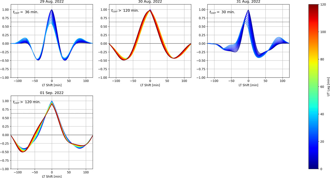
Figure 10. Same as Figure 9 but for 2022 campaign.

It can be seen that $t_{\mathit{corr}}$ is highly variable on a night-to-night basis. Only two of the nine campaign nights show $t_{\mathit{corr}}>$ 120 min, although it should be noted that two other nights (21 Sept. 2021 and 23 Sept. 2021) exhibit strong correlation over at least 104 min. The nights with short correlation times (less than 2 h) have $t_{\mathit{corr}}$ ranging from 114 min to as little as 24 min. In particular, one of the shortest correlation times occurred on 29 Aug. 2022, which is one of the nights when WAM-IPE electric fields prevented the growth of irregularities in the regional simulation. Although the autocorrelation functions shown for each dataset cannot be compared directly, a general understanding of $t_{\mathit{corr}}$ can be gathered from both. The occasional short correlation times in WAM-IPE estimates are contradictory to the regularly observed long correlation times seen in ICON data. There does not appear to be a connection between correlation time and accuracy of the resulting regional simulations. This is evident due to 29 Aug. 2022 having a small $t_{\mathit{corr}}$ value while 01 Sept. 2022 exhibits a large value of $t_{\mathit{corr}}$, yet both nights were missed detections when the simulation was driven with WAM-IPE electric fields. On the other hand, 30 Aug. 2022 shows a large $t_{\mathit{corr}}$ and 31 Aug. 2022 has a short $t_{\mathit{corr}}$ while both nights had accurate simulations of absent ESF.

5 Conclusion

The regional simulation described in Section 2 is capable of reproducing night-to-night observations of ESF activity when initialized and driven by proper observational data. Most importantly, the simulation is sensitive to the strength, duration, and timing of the PRE. Previous results of the simulation indicate that the most reliable method of determining background electric fields is to derive them from ISR-measured vertical plasma drifts. This, however, is not a true forecast as it relies on real-time radar measurements to reproduce irregularities that are actively present and not about to develop. Additionally, the simulation has a very high computational cost and is unable to run in real time. In an attempt to move towards a true forecast using the simulation, predicted background electric fields taken from WAM-IPE were used to drive the simulation. These attempts were less successful than the ISR-driven results as missed detections were recorded. The lack of night-to-night accuracy in WAM-IPE background electric fields is capable of suppressing instabilities and may also be capable of generating artificial instabilities in the regional simulation.

To analyze the background electric fields from WAM-IPE, a proxy electrodynamics model was developed and used to perform a variety of sensitivity tests. Multiple sensitivities of the dynamo solver were tested related to the ionospheric composition and neutral wind structure. Replacing WAM-IPE winds with HWM14 appeared to improve agreement between the resulting electric fields and ISR observations for some nights, but not others. Other sensitivities tested also did not improve the agreement. These results suggest that there is not a simple substitution or scaling of WAM-IPE parameters that would produce electric fields comparable to ISR observations on a night-to-night basis.

While no sensitivity tests reproduced ISR observations, they did appear to significantly impact the resulting electric fields. In agreement with [31] the PRE appears to rely on the global wind patterns rather than local patterns surrounding the terminator. This highlights the importance of thermospheric wind observations for a potential ESF forecast. [20] suggested disagreement between WAM-IPE and HWM14 thermospheric winds that may also prove detrimental to the resulting electrodynamics. Further exploration and validation of global WAM-IPE neutral wind patterns may improve the day-to-day accuracy of its equatorial electrodynamics estimations.

Additionally, the vertical plasma drifts produced by WAM-IPE electric fields were compared to those measured by the ICON satellite. In particular, we note that ICON data agrees with the theory that the global structure of the vertical drifts and the PRE maintain their shape and vary slowly. As measured by ICON the PRE appears to have a correlation time of at least 104 min In contrast, it was shown that WAM-IPE results may vary the PRE structure rapidly with correlation times dropping to as little as 20 min. Further work is needed to understand the effect of a persistent, or rapidly changing, PRE on ESF development and the growth of irregularities in the regional simulation.

A multitude of factors can affect the growth of irregularities associated with ESF. Contemporary results suggest that the most important of these factors are the background electric fields, the strength and timing of the PRE, and the neutral thermospheric winds that produce the ionospheric dynamo. A true forecast of ESF must capture each of these factors, and others, accurately on a night-to-night basis. Improvement of the night-to-night accuracy in WAM-IPE electric fields is critical to the model acting as the baseline for a regional forecast. Currently, the electric fields predicted by WAM-IPE do no better than climatology and are therefore unable to drive a forecast that is more accurate than climatology. Further sensitivity tests, may indicate additional sources for more accurate variability in the WAM-IPE electric fields.

Data availability statement

The datasets presented in this study can be found in online repositories. The names of the repository/repositories and accession number(s) can be found in the article/Supplementary Material.

Author contributions

AK: Investigation, Methodology, Writing–original draft, Writing–review and editing, Conceptualization, Formal Analysis. DH: Conceptualization, Funding acquisition, Investigation, Methodology, Supervision, Writing–review and editing, Formal Analysis. T-WF: Data curation, Writing–review and editing, Supervision.

Funding

The author(s) declare that financial support was received for the research, authorship, and/or publication of this article. This project is supported by NSF award no. AGS-2028032 to Cornell University and the University of Colorado Boulder. The Jicamarca Radio Observatory is a Instituto Geofisico del Peru facility operated with support from NSF award no. AGS-1732209 through Cornell University.

Acknowledgments

The authors thank Tim Fuller-Rowell for his help in interpreting WAM-IPE data. We also thank the Jicamraca Radio Observatory staff for their help in collecting radar data.

Conflict of interest

The authors declare that the research was conducted in the absence of any commercial or financial relationships that could be construed as a potential conflict of interest.

The author(s) declared that they were an editorial board member of Frontiers, at the time of submission. This had no impact on the peer review process and the final decision.

Publisher’s note

All claims expressed in this article are solely those of the authors and do not necessarily represent those of their affiliated organizations, or those of the publisher, the editors and the reviewers. Any product that may be evaluated in this article, or claim that may be made by its manufacturer, is not guaranteed or endorsed by the publisher.

Supplementary material

The Supplementary Material for this article can be found online at: https://www.frontiersin.org/articles/10.3389/fphy.2024.1488935/full#supplementary-material

References

1. Booker HG, Wells HW. Scattering of radio waves by the F-region of the ionosphere. Terrestrial Magnetism Atmos Electricity (1938) 43:249–56. doi:10.1029/TE043i003p00249

CrossRef Full Text | Google Scholar

2. Woodman RF, La Hoz C. Radar observations of F region equatorial irregularities. J Geophys Res (1896-1977) (1976) 81:5447–66. doi:10.1029/JA081i031p05447

CrossRef Full Text | Google Scholar

3. Zargham S, Seyler CE. Collisional interchange instability: 1. Numerical simulations of intermediate-scale irregularities. J Geophys Res Space Phys (1987) 92:10073–88. doi:10.1029/JA092iA09p10073

CrossRef Full Text | Google Scholar

4. Kelley MC, Seyler CE, Zargham S. Collisional interchange instability: 2. A comparison of the numerical simulations with the in situ experimental data. J Geophys Res Space Phys (1987) 92:10089–94. doi:10.1029/JA092iA09p10089

CrossRef Full Text | Google Scholar

5. Hysell DL, Kudeki E. Collisional shear instability in the equatorial F region ionosphere. J Geophys Res Space Phys (2004) 109. doi:10.1029/2004JA010636

CrossRef Full Text | Google Scholar

6. Woodman RF. Spread F – an old equatorial aeronomy problem finally resolved? Ann Geophysicae (2009) 27:1915–34. doi:10.5194/angeo-27-1915-2009

CrossRef Full Text | Google Scholar

7. Kelley MC, Makela JJ, de La Beaujardière O, Retterer J. Convective ionospheric storms: a review. Rev Geophys (2011) 49. doi:10.1029/2010RG000340

CrossRef Full Text | Google Scholar

8. Haerendel G. Theory of equatorial spread F. Max Planck Institute for extraterrestrial Physics (1973).

Google Scholar

9. Sultan PJ. Linear theory and modeling of the Rayleigh-Taylor instability leading to the occurrence of equatorial spread F. J Geophys Res Space Phys (1996) 101:26875–91. doi:10.1029/96JA00682

CrossRef Full Text | Google Scholar

10. Scannapieco AJ, Ossakow SL. Nonlinear equatorial spread F. Geophys Res Lett (1976) 3:451–4. doi:10.1029/GL003i008p00451

CrossRef Full Text | Google Scholar

11. Hysell DL, Jafari R, Milla MA, Meriwether JW. Data-driven numerical simulations of equatorial spread F in the Peruvian sector. J Geophys Res Space Phys (2014) 119:3815–27. doi:10.1002/2014JA019889

CrossRef Full Text | Google Scholar

12. Hysell DL, Kirchman A, Harding BJ, Heelis RA, England SL. Forecasting equatorial ionospheric convective instability with ICON satellite measurements. Space Weather (2023) 21:e2023SW003427. doi:10.1029/2023SW003427

CrossRef Full Text | Google Scholar

13. Hysell DL, Kirchman A, Harding BJ, Heelis RA, England SL, Frey HU, et al. Using ICON satellite data to forecast equatorial ionospheric instability throughout 2022. Space Weather (2024) 22. doi:10.1029/2023SW003817

CrossRef Full Text | Google Scholar

14. Fejer BG, Scherliess L, de Paula ER. Effects of the vertical plasma drift velocity on the generation and evolution of equatorial spread F. J Geophys Res Space Phys (1999) 104:19859–69. doi:10.1029/1999JA900271

CrossRef Full Text | Google Scholar

15. Rishbeth H. The F-region dynamo. J Atmos Terrestrial Phys (1981) 43:387–92. doi:10.1016/0021-9169(81)90102-1

CrossRef Full Text | Google Scholar

16. Farley DT, Bonelli E, Fejer BG, Larsen MF. The prereversal enhancement of the zonal electric field in the equatorial ionosphere. J Geophys Res Space Phys (1986) 91:13723–8. doi:10.1029/JA091iA12p13723

CrossRef Full Text | Google Scholar

17. Eccles JV. A simple model of low-latitude electric fields. J Geophys Res Space Phys (1998) 103:26699–708. doi:10.1029/98JA02657

CrossRef Full Text | Google Scholar

18. Eccles JV, St. Maurice JP, Schunk RW. Mechanisms underlying the prereversal enhancement of the vertical plasma drift in the low-latitude ionosphere. J Geophys Res Space Phys (2015) 120:4950–70. doi:10.1002/2014JA020664

CrossRef Full Text | Google Scholar

19. Scherliess L, Fejer BG. Radar and satellite global equatorial F region vertical drift model. J Geophys Res Space Phys (1999) 104:6829–42. doi:10.1029/1999JA900025

CrossRef Full Text | Google Scholar

20. Hysell DL, Fang TW, Fuller-Rowell TJ. Modeling equatorial F -region ionospheric instability using a regional ionospheric irregularity model and WAM-IPE. J Geophys Res Space Phys (2022) 127. doi:10.1029/2022JA030513

CrossRef Full Text | Google Scholar

21. Fang T-W, Fuller-Rowell T, Kubaryk A, Li Z, Millward G, Montuoro R. Operations and recent development of NOAA’s Whole. Atmosphere Model (2022) 44:849.

Google Scholar

22. Maruyama N, Sun Y-Y, Richards PG, Middlecoff J, Fang T-W, Fuller-Rowell TJ, et al. A new source of the midlatitude ionospheric peak density structure revealed by a new Ionosphere-Plasmasphere model. Geophys Res Lett (2016) 43:2429–35. doi:10.1002/2015GL067312

CrossRef Full Text | Google Scholar

23. Swisdak M. Notes on the dipole coordinate system. (2006).

Google Scholar

24. Wohlwend CS. Modeling the electrodynamics of the low-latitude ionosphere. Utah State University (2008) Ph.D. thesis.

Google Scholar

25. Schunk R, Nagy A. Ionospheres: physics, plasma physics, and chemistry. Cambridge, Cambridge University Press (2004).

Google Scholar

26. Richmond AD. Ionospheric electrodynamics using magnetic apex coordinates. J geomagnetism geoelectricity (1995) 47:191–212. doi:10.5636/jgg.47.191

CrossRef Full Text | Google Scholar

27. Laundal KM, Richmond AD. Magnetic coordinate systems. Space Sci Rev (2017) 206:27–59. doi:10.1007/s11214-016-0275-y

CrossRef Full Text | Google Scholar

28. Alken P, Thébault E, Beggan CD, Amit H, Aubert J, Baerenzung J, et al. International geomagnetic reference field: the thirteenth generation. Earth, Planets and Space (2021) 73:49. doi:10.1186/s40623-020-01288-x

CrossRef Full Text | Google Scholar

29. Farley DT. A theory of electrostatic fields in the ionosphere at nonpolar geomagnetic latitudes. J Geophys Res (1896-1977) (1960) 65:869–77. doi:10.1029/JZ065i003p00869

CrossRef Full Text | Google Scholar

30. Eccles JV. The effect of gravity and pressure in the electrodynamics of the low-latitude ionosphere. J Geophys Res Space Phys (2004) 109. doi:10.1029/2003JA010023

CrossRef Full Text | Google Scholar

31. Richmond AD, Fang T-W, Maute A. Electrodynamics of the equatorial evening ionosphere: 1. Importance of winds in different regions. J Geophys Res Space Phys (2015) 120:2118–32. doi:10.1002/2014JA020934

CrossRef Full Text | Google Scholar

32. Emmert JT, Richmond AD, Drob DP. A computationally compact representation of Magnetic-Apex and Quasi-Dipole coordinates with smooth base vectors. J Geophys Res Space Phys (2010) 115. doi:10.1029/2010JA015326

CrossRef Full Text | Google Scholar

33. Heelis R. Icon ion velocity meter (ivm) a data. (2023) doi:10.48322/2mv5-xy46

CrossRef Full Text | Google Scholar