Physics of the Edwards–Anderson spin glass in dimensions d = 3, … ,8 from heuristic ground state optimization

We present a collection of simulations of the Edwards–Anderson lattice spin glass at $T=0$ to elucidate the nature of low-energy excitations over a range of dimensions that reach from physically realizable systems to the mean-field limit. Using heuristic methods, we sample the ground states of instances to determine their energies while eliciting excitations through manipulating boundary conditions. We exploit the universality of the phase diagram of bond-diluted lattices to make such a study in higher dimensions computationally feasible. As a result, we obtain a variety of accurate exponents for domain wall stiffness and finite-size corrections, which allow us to examine their dimensional behavior and their connection with predictions from mean-field theory. We also provide an experimentally testable prediction for the thermal-to-percolative crossover exponent in dilute lattice Ising spin glasses.

1 Introduction

Imagining physical systems in non-integer dimensions, such as through $\epsilon$-expansion [1] or dimensional regulation [2], to name but two, has provided many important results for the understanding of physics in realistic dimensions. For example, the goal of the $\epsilon$-expansion is to establish a connection between the (technically, infinite-dimensional) mean-field solution of a field theory and its real-space behavior. For a disordered system such as a spin glass [3–6], this playbook has proved rather difficult to follow theoretically [7–9]. In contrast, we endeavor to explore the transition between the often well-known mean-field properties and their modifications in real space using numerical means, free of any theoretical preconceptions. In this task, on top of the computationally extensive disorder averages, the complexity of spin glasses reveals itself through increasingly slower convergence in thermal simulations, while the deeper one pushes into the glassy regime. Going all the way to $T=0$ then makes thermal explorations impossible and renders the problem of finding the ground-state NP-hard in general [10]. However, simulations at $T=0$ also avail us considerable conceptual clarity and an entirely new suit of techniques, albeit for just a few, yet important, observables. Some equilibrium properties of spin glasses below $T_c$ can be obtained from merely determining ground-state energies, such as domain wall stiffness, finite-size corrections, and thermal–percolative crossover exponents. To keep systematic errors low while also creating enough statistics for the disorder average, we need to use fast but ultimately inexact heuristic methods to overcome NP-hardness. To reach a sensible scaling regime in system sizes, $N$, especially in higher dimensions, requires clever exploitation of the phase diagram of a spin glass. In this study, we discuss the results obtained from large-scale simulations conducted over several years and spread over a number of papers [11–15].¹

To be specific, we simulate the Ising spin glass model due to Edwards and Anderson (EA) with the Hamiltonian [16].

$H=-{\displaystyle \sum _{<i,j>}}{J}_{i,j}{\sigma }_i{\sigma }_j.(1)$

The dynamic variables are binary (Ising) spins ${\sigma }_i=\pm 1$ placed on a hypercubic lattice in the integer $d$ dimension with couplings between nearest neighbors $<i,j>$ via random bonds $J_{ij}$ drawn from some distribution $\mathcal{P}(J)$ of zero mean and unit variance. The lattices are periodic with base length $L$ in all directions, i.e., each such instance has $N=L^d$ spins. To relate real-world behavior in $d=3$ (which is explored experimentally and theoretically in other articles in this collection) with mean-field behavior, which manifests itself above the upper critical dimension $d_u=6$ [3], we found ground states of EA on lattices in $d=3,\dots ,8$. In each $d$, we need to simulate instances over a wide range of $L$ to extrapolate our results to the thermodynamic limit $(L\to \infty )$. At each size $L$, we further need to measure a large number of instances with independently drawn random bonds for the disorder average inherent to obtain observables in spin glasses. Each instance entails approximating its ground state, which is an NP-hard combinatorial problem.

To sample ground-state of the Hamiltonian in Equation 1 at high throughput and with minimal systematic errors, heuristics can only be relied on for systems with not more than $N\approx 1000$ spins coupled together. This would appear to limit the “dynamic range” in size up to approximately $L=10$ in $d=3$ but limited to $L=6$ in $d=4$, and even to $L<3$ in $d=7$, definitely insufficient to extract any $L\to \infty$ limit. However, the phase diagram for a bond-diluted EA system (with $d\ge 3$ such that $T_c>0$) shown in Figure 1 suggests that universal scaling behavior extends across the entire spin-glass (SG) phase down to the scaling window near the bond-percolation threshold $p_c$ for low enough $T$, i.e., most definitely for $T=0$. Thus, our strategy is to find ground states for EA instances at bond density $p$ with sufficient dynamic ranges in $L$ for $p>p_c$ just above that scaling window to be within the SG phase, using exact reduction methods [12, 17] (see Supplementary Appendix SA) to remove a large number of spins, followed by heuristic optimization of remainder systems with $N_r\le 1000$ [18, 19] (see Supplementary Appendix SB). These reduction methods recursively trace out all spins with fewer than four connected neighbors, at least, and are particularly effective near $p_c$ since each spin in the EA system has at most $2d$ potential neighbors while $p_c\sim 1/(2d)$ in large $d$ such that for $p$ just above $p_c$, lattices remain sparse, each spin being connected to barely more than one other spin, on average, albeit with large variations. For example, in $d=8$ for $p=0.0735>p_c\approx 0.068$ and $L=6$, an EA system with $N=6^8\approx 1.7\times 10^6$ spins typically reduces to a remainder graph with $⟨N_r⟩\approx 1000$ spins, each connected to 5.3 neighbors, on average, to be optimized heuristically.

Figure 1

Figure 1. Phase diagram for bond-diluted spin glasses $(d>d_l)$. The entire spin-glass (SG) phase for $T<T_c$ and $p>p_c$ has a universal positive domain wall exponent, $y>0$. In our measurements, we therefore utilize an interval of bond densities at $T=0$ (red arrow) where $p$ is sufficiently above the scaling window near $p_c$ (at finite system size) but small enough to asymptotically reach significant system sizes $L$. At $p=p_c$ and $T=T_c=0$, we define the domain wall exponent for a spin glass on the percolating cluster as $y=y_P(<0)$. It allows us to extract the thermal–percolative crossover exponent $\varphi$ that describes the behavior along the boundary $T_c(p)\sim {(p-p_c)}^{\varphi }$ for $p\searrow p_c$ (green arrow). In the paramagnetic phase (PM) for $p<p_c$ or $T>T_c$, defect energies due to domain walls decay exponentially.

2 Domain wall stiffness exponents

A quantity of fundamental importance for the modeling of amorphous magnetic materials through spin glasses [3, 20–23] is the domain wall or “stiffness” exponent $y$, often also labeled $\theta$. As Hook’s law describes the response to increasing elastic energy imparted to a system for increasing displacement $L$ from its equilibrium position, the stiffness of a spin configuration describes the typical increase in magnetic energy $\mathrm{\Delta }E$ due to an induced defect interface of a domain of size $L$. However, unlike uniform systems with a convex potential energy function over its configuration space (say, a parabola for the single degree of freedom in Hook’s law, or a high-dimensional funnel for an Ising ferromagnet), an amorphous many-body system exhibits a function more reminiscent of a high-dimensional mountain landscape. Any defect-induced displacement of size $L$ in such a complicated energy landscape may move a system through numerous undulations in energy $\mathrm{\Delta }E$. Averaging over many incarnations of such a system results in a typical energy scale

$\sigma \left(\mathrm{\Delta }E\right)\sim L^y\left(L\to \infty \right)(2)$

for the standard deviations of the domain wall energy $\mathrm{\Delta }E$.

The importance of this exponent for small excitations in disordered spin systems has been discussed in many contexts [22, 24–28]. Spin systems with $y>0$ provide resistance (“stiffness”) against the spontaneous formation of defects at sufficiently low temperatures $T$, an indication that a phase transition $T_c>0$ to an ordered state exists. For instance, in an Ising ferromagnet, the energy $\mathrm{\Delta }E$ is always proportional to the size of the interface, i.e., $y=d-1$, which is consistent with the fact that $T_c>0$ only when $d>1$. For $y<0$, the state of a system is unstable with respect to defects, and spontaneous fluctuations may proliferate, preventing any ordered state. Thus, determining the exact “lower critical dimension” $d_l$, where $y{|}_{d=d_l}=0$, is of singular importance, and understanding the mechanism leading to $d_l$, however unnatural its value, provides clues to the origin of order [13, 29–33].

Instead of waiting for a thermal fluctuation to spontaneously induce a domain wall, it is expedient to directly impose domains of size $L$ through reversed boundary conditions on the system and measure the energy needed to determine $y$. To wit, in a system with periodic boundary conditions, we first obtain its ground state $E_0$ unaltered and obtain it again as $E_0^{\prime }$ after reversing the signs on all bonds within a $(d-1)$-dimensional hyperplane, resulting in a complex domain of spins of size $\sim L$ that are reversed between both ground states such that $\mathrm{\Delta }E=E_0-E_0^{\prime }$ is the energy due to the interface of that domain. Since $\mathrm{\Delta }E$ is equally likely to be positive or negative, it is its deviation, $\sigma (\mathrm{\Delta }E)$, which sets the energy scale in Equation 2. Notably, this problem places an even higher demand on the ground-state heuristic than described in the introduction. Here, the domain wall energy $\mathrm{\Delta }E$ has a minute, sub-extensive difference between two almost identical, extensive energies, $E_0$ and $E_0^{\prime }$, each of which is NP-hard to find. Thus, any systematic error would escalate rapidly with $N_r$, the size of the remainder graph.

As shown in Figure 2, using bond-diluted lattices for the EA system, in contrast, not only affords us a larger dynamic range in $L$ but also allows for an extended scaling regime due to the additional parameter of $p$ ranging over an entire interval. Instead of one set of data for increasing $L$ at a fixed $p$ (typically, $p=1$ [34]) leading to the scaling in Equation 2, we can scale multiple independent sets for such a range of $p$ into a collective scaling variable, $\mathcal{L}=L{\left(p-p^{*}\right)}^{\nu }$, which collapses the data according to $\sigma (L,p)\sim {\mathcal{L}}^y$. Although the extension to an interval in $p$ makes simulations more laborious, it typically yields an extra order of magnitude in scaling compared to the prohibitive effort of confronting the NP-hard problem of reaching large $L$ at fixed $p$ alone. For instance, in $d=3$ at $p=1$, attainable sizes span $3\le L\le 12$, at best, while we obtain a perfect data collapse for about $0.07\le \mathcal{L}\le 3$ for $0.28\le p\le 0.8$ (note that while $p^{*}\approx p_c$ and $\nu$ has some relation to the correlation-length exponent in percolation [see below], it is necessary to allow these to be a free parameter for the bimodal bonds used in these simulations, as was argued by [12]). The fitted values for $y$ for each $d$, as obtained from Figure 2, are listed in Table 1.

Figure 2

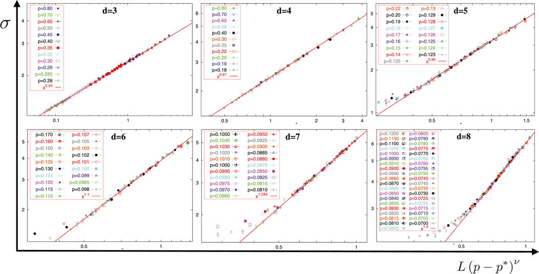
Figure 2. Data collapse for the domain wall scaling simulations of bond-diluted EA in $d=3,\dots ,8$ of $\sigma (L,p)\sim {\mathcal{L}}^y$ in the scaling variable $\mathcal{L}=L{\left(p-p^{*}\right)}^{\nu }$. For each $d$, datasets are created over a range in $p$ as listed in the respective legend, up to a size $L$ such that remainder graphs are typically $<⟨N_r⟩\approx 10^3$. The original data and the fitting parameters are listed in [11, 12]. The obtained domain wall scaling exponents $y_d$ are listed in Table 1. Note that for $d\le 6$, transient data for smaller $\mathcal{L}$ have been omitted for clarity.

Table 1

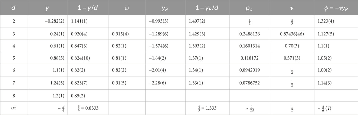
Table 1. Stiffness exponents for Edwards–Anderson spin glasses [11, 12] for dimensions $d=2,\dots ,8$ obtained numerically from domain wall excitations of ground states, as shown in Figure 2. The next column contains the measured values for finite-size corrections, denoted as $\omega$, from the fit of the data shown in Figure 3. The stiffness exponents $y_P$ obtained by [14] refer to EA at the bond–percolation threshold $p_c$, with values of $p_c$ obtained from [36] for $d=3$ and [37] for $d\ge 4$. The correlation–length exponents $\nu$ for percolation are from [38] in $d=3$ and from [39] for $d\ge 4$, where $\nu =1/2$ is exactly above the upper critical dimension, $d\ge 6$.

The values for $y$ are listed in Table 1 and plotted in Figure 4 as $1-\frac{y}{d}$. That quantity has been obtained in the mean-field case by [35], yielding $1-\frac{y}{d}=\frac{5}{6}$ above the upper critical dimension, $d\ge d_u=6$. That value is clearly consistent with our high-dimensional data, providing a rare direct comparison between the mean field theory (RSB) and real-world spin glasses. As shown in Figure 4, the exponent varies continuously with dimension $d$ and allows for a simple cubic fit of the numerical data between $2\le d\le 6$, weighted by the statistical errors [13]. The fit independently reproduces the exact known result outside the fitted domain at $d=1$, $y=-1$, to less than $0.8\%$ (not shown here). The fit has a zero at $d_l\approx 2.498$ and yields $y\approx 0.001$ at $d=\frac{5}{2}$; there is strong evidence that $d_l=5/2$, which has also been suggested by theory [30, 33] and is consistent with the experiment [32].

In the following section, we consider some other uses of the domain wall excitations.

3 Ground-state finite-size correction exponents

Since simulations of statistical systems are bound to be conducted at system sizes $N$ typically quite far from the thermodynamic limit $N\to \infty$, it becomes essential to understand the corrections entailed by such limitations. This is especially pertinent for spin glasses beset with extra complexities such as NP-hardness at $T=0$ (or, similarly, the lack of equilibration at low but finite $T$) or the additional burden of disorder averaging over many random samples severely limiting $N$. Only rarely do such corrections decay fast enough to reveal the thermodynamic behavior of an observable in a simulation at a single, “large enough” $N$. Instead, as already observed for the stiffness in Section 2, typically, sets of data need to be generated to glean the asymptotic behavior for large sizes. To extrapolate the value of an intensive observable (like the ground-state energy density), it is then necessary to have a handle on the nature of the finite-size corrections (FSCs) that have to be expected for the generated data [25, 40, 41]. However, FSCs are not only a technical necessity. Their behavior is often closely related to other physical properties in the thermodynamic limit via scaling relations [27]. They can also be instrumentalized, for instance, to assess the scalability of optimization heuristics [42, 43].

For the ground-state energy densities in the EA system, [27] argued that such FSCs should be due to locked-in domain walls of energy $\sim L^y$, which would lead to the scaling correction for the extensive energies of $E_L\sim e_{\infty }{L}^d+\mathrm{\Upsilon }{L}^y$ for large $L$, defining $e_{\infty }$ as the $L\to \infty$ limit of the average ground-state energy density $e_L=⟨\frac{E_L}{L^d}⟩$. This is consistent with Equation 2, where we purposefully created such a domain wall because the same system freed from that domain wall (or locked into another one) would have $E_L^{\prime }\sim e_{\infty }{L}^d+{\mathrm{\Upsilon }}^{\prime }{L}^y$ and, thus, $\mathrm{\Delta }{E}_L\sim \mathrm{\Delta }\mathrm{\Upsilon }{L}^y$. Dividing $E_L$ by system size, we obtain

$e_L\sim e_{\infty }+\frac{A}{{\left(L^d\right)}^{\omega }},\left(L\to \infty \right),(3)$

where the FSC exponent is conjectured to be

$\omega =1-\frac{y}{d}.(4)$

Indeed, our direct evaluation of ground-state energy densities at some fixed bond density $p$ in dimensions $d=3,\dots ,7$, as shown in Figure 3, is convincingly in agreement with this picture for the dominant contributions to FSCs. However, that leaves us with somewhat of a conundrum when compared with mean-field simulations, where FSCs for the Sherrington–Kirkpatrick (SK) spin glass model [44–46] appear to yield $\omega \approx \frac{2}{3}$ for $d\to \infty$, which is not close to $1-y/d\to \frac{5}{6}$ from RSB theory [35].

Figure 3

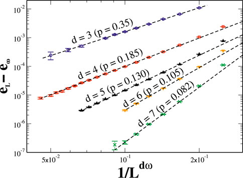
Figure 3. Plot of finite-size corrections to ground-state energies in bond-diluted lattice spin glasses (EA). For each dimension $d$, ground-state averages $e_L$ at increasing system sizes $L$ were obtained at a convenient bond density $p$. An asymptotic fit (dashed lines) of those data according to Equation 3 was obtained. The resulting values for the finite-size correction exponent $\omega$ are listed in Table 1 and plotted as shown in Figure 4, suggesting that Equation 4 holds.

We conducted a corresponding ground-state study at the edge of the SG regime (see Figure 1) by choosing the percolation point $p=p_c$ exactly. Since the fractal percolation cluster cannot sustain an ordered state, we found that the stiffness exponent defined in Equation 2 is negative there, $y{|}_{p=p_c}=y_P<0$. Numerical studies of ground states at $p_c$ (using Gaussian bonds $J_{ij}$ in this case) are computationally quite efficient since the fractals embedded in the lattice often reduce completely or so substantially that heuristics produce little systemic error. Large lattice sizes $L$ can be achieved, limited only by rare large remainder graphs or the lack of memory needed to build the original, unreduced EA lattice. The values for $y_P$ thus obtained [14] are also listed in Table 1. Although the hypothesis for FSCs from Equation 4, $\omega =1-y_P/d$, leads to large values for $\omega$ when $y_P<0$ and it becomes hard to test numerically, the corrections found are well consistent with the hypothesis [15]. In particular, it appears that $1-y_P/d\to \frac{4}{3}$ for $d\ge d_u=6$, which would be consistent with FSCs in percolating random graphs [47]. Although this provides an argument that Equation 4 should also hold in the mean-field limit for the EA system in the spin glass phase, the SK model might be a poor representation of that limit for the EA system. In the EA system, we first let $L\to \infty$ for a fixed number of neighbors $2dp$ before $d\to \infty$, while in the SK model, both system size and neighborhood diverge simultaneously. Unfortunately, sparse mean-field spin glasses on regular graphs (“Bethe lattices”) appear to have FSCs with $\omega =\frac{2}{3}$ [48], but those results might depend, to some extent, on the structural details of the mean-field networks [45, 49, 50], and which structure most closely resembles a mean-field version of EA at $d\to \infty$ remains unclear.

4 Thermal–percolative crossover exponents

Having already determined the percolative stiffness exponents $y_P$ in the previous section, we can utilize it to make an interesting—and potentially experimentally testable—prediction about the behavior of the phase transition line, as shown in Figure 1. For diluted lattices at variable bond density $p\to p_c$, Equation 2 generalizes to [51, 52]

$\sigma {\left(\mathrm{\Delta }E\right)}_{L,p}\sim \mathcal{Y}\left(p\right)L^{y}f\left(L/\xi \left(p\right)\right).(5)$

Here, we assume that $\mathcal{Y}(p)\sim {(p-p_c)}^t\sim {\xi }^{-t/\nu }$ for the surface tension and $\xi (p)\sim {(p-p_c)}^{-\nu }$ is the conventional correlation length for percolation. The scaling function $f$ is defined to be constant for $L\gg \xi (p)\gg 1$, where percolation (and hence, $\xi$) plays no role, and we regain Equation 2 for $p>p_c$. For $\xi \gg L\gg 1$, Equation 5 requires $f(x)\sim x^{\mu }$ for $x\to 0$ to satisfy $\sigma \to 0$ with some power of $L$, needed to cancel the $\xi$ dependence at $p=p_c$. Thus, $\mu =-t/\nu$, and we obtain $y_P=y+\mu =y-t/\nu$ to mark the $L$ dependence of $\sigma$ at $p=p_c$, as mentioned before, which yields $t=\nu (y-y_P)$. Finally, at the crossover $\xi \sim L$, where the range $L$ of the excitations $\sigma (\mathrm{\Delta }E)$ reaches the percolation length beyond which spin glass order ensues, Equation 5 provides

$\sigma {\left(\mathrm{\Delta }E\right)}_{\xi \left(p\right),p}\sim {\left(p-p_c\right)}^t\xi {\left(p\right)}^{y}f\left(1\right)\sim {\left(p-p_c\right)}^{-\nu y_P}.(6)$

Associating a temperature with the energy scale of the crossover in Equation 6 by $\sigma {(\mathrm{\Delta }E)}_{\xi (p),p}\sim T_c$ (since, for $T>T_c$, thermal fluctuations destroy order at a length-scale $\ll \xi$) leads to

$T_g\left(p\right)\sim {\left(p-p_c\right)}^{\varphi },\mathrm{w}\mathrm{i}\mathrm{t}\mathrm{h}\varphi =-\nu y_P,(7)$

defining [51] the “thermal–percolative crossover exponent” $\varphi$. All data for $d=2,\dots ,7$ are listed in Table 1, and the results for $\varphi$ are also shown in Figure 4. It appears that $\varphi$ decreases with increasing $d$ for $d\le d_u=6$, has a minimum of $\varphi =1$ at $d_u=6$, and increases as $\varphi =d/6$ above $d_u$.

Figure 4

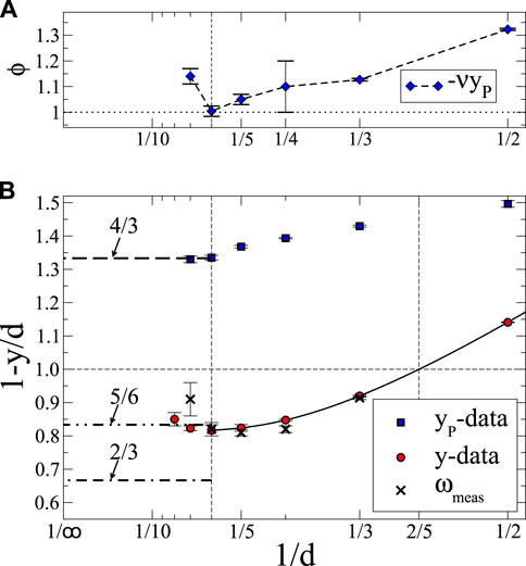
Figure 4. Plot summarizing the data for the exponents in Table 1, here plotted as a function of inverse dimension, $1/d$, to highlight the connection with the mean field limit for $d\ge d_u=6$ (left vertical line). (B) refers to the stiffness exponents $y$ in the spin-glass regime (SG in Figure 1) or $y_P$ at $p_c$ and $T=0$, each presented as $1-y/d$. Included are also the measured FSC exponents $\omega$, which appear to be consistent with the conjecture in Equation 4. For stiffness, the $y$ data are quite consistent with $1-y/d=5/6$ predicted for $d\ge d_u$ [35] but not with the FSC ${\omega }_{\text{SK}}=2/3$ found for SK [44]. The fit of this data (solid line) yields a lower critical dimension $d_l\approx \frac{5}{2}$, where $y=0$ (right vertical line). At $p_c$, the $y_P$ data appear to approach a value of $\omega =4/3$ expected for the FSCs of percolating random graphs. In (A), $y_P$ is multiplied with the independent percolation exponent $\nu$to form the thermal–percolative crossover exponent $\varphi$ that characterizes the behavior of the phase boundary near $p_c$ in Equation 7, see green arrows in Figure 1. It seems to show a minimum of $\varphi \approx 1$ at $d=d_u=6$.

Of particular experimental interest is the result for $d=3$, $y_P=-1.289(6)$, predicting $\varphi =1.127(5)$ with $\nu =0.87436(46)$ [38]. This exponent provides a non-trivial, experimentally testable prediction derived from scaling arguments of equilibrium theory at low temperatures (since bond and site percolation are typically in the same universality class, it should make little difference whether an experiment varies the site concentration of atoms with dipolar spin or the bonds between them). Such tests are few as disordered materials by their very nature fall out of equilibrium when entering the glassy state. The phase boundary itself provides the perfect object for such a study. It can be approached by theory from below and by experiments from above where equilibration is possible. [53] already provided highly accurate results for the freezing temperature $T_M$ as a function of dilution $x$ for a doped, crystalline glass, (${\mathrm{L}\mathrm{a}}_{1-x}$Gd_x)₈₀${\mathrm{A}\mathrm{u}}_{20}$, proposing a linear dependence, $T_M\sim x$. The tabulated data are equally well fitted using Equation 7 in that regime. [54] determined a phase diagram for ${({\mathrm{F}\mathrm{e}}_x{\mathrm{N}\mathrm{i}}_{1-x})}_{75}{\mathrm{P}}_{16}{\mathrm{B}}_6{\mathrm{A}\mathrm{l}}_4$, an amorphous alloy, for a wide range of temperatures $T$ and site concentrations $x$ but did not discuss its near-linear behavior at low $x$. A similar phase diagram for the insulator ${\mathrm{C}\mathrm{d}\mathrm{C}\mathrm{r}}_{2x}$In_2(1-x)S₄ is shown in Figure 1A of [55]. New experiments dedicated to the limit $x\searrow x_c$ should provide the results of sufficient accuracy to test our prediction for $\varphi$.

5 Conclusions

We summarized a collection of simulation data pertaining to the lattice spin glass EA over a range of dimensions, providing a comprehensive description of low-energy excitations from experimentally accessible systems to the mean-field level, where exact results can be compared with. Putting all those results side-by-side paints a self-consistent picture of domain wall excitations, their role in the stability of the ordered glass state, and their role for finite-size corrections. Extending to the very physical concept of bond density made simulations in high dimensions feasible, added accuracy, and opened up the spin-glass phase diagram, which makes new observables experimentally accessible, such as the thermal–percolative crossover exponent.

Going forward, the methods developed here could be extended to study, say, ground-state entropy and their overlaps [56] or the fractal nature of domain walls [57, 58]. Our method might also inspire new ways of using dilution as a gadget to make simulations more efficient [59].

Author contributions

SB: conceptualization, data curation, formal analysis, investigation, methodology, writing–original draft, and writing–review and editing.

Funding

The author(s) declare that no financial support was received for the research, authorship, and/or publication of this article.

Conflict of interest

The author declares that the research was conducted in the absence of any commercial or financial relationships that could be construed as a potential conflict of interest.

Publisher’s note

All claims expressed in this article are solely those of the authors and do not necessarily represent those of their affiliated organizations, or those of the publisher, the editors, and the reviewers. Any product that may be evaluated in this article, or claim that may be made by its manufacturer, is not guaranteed or endorsed by the publisher.

Supplementary material

The Supplementary Material for this article can be found online at: https://www.frontiersin.org/articles/10.3389/fphy.2024.1466987/full#supplementary-material

Footnotes

¹http://www.physics.emory.edu/faculty/boettcher

References

1. Wilson KG, Fisher ME. Critical exponents in 3.99 dimensions. Phys Rev Lett (1972) 28:240–3. doi:10.1103/physrevlett.28.240

CrossRef Full Text | Google Scholar

2. t’Hooft G, Veltman MJG. Regularization and renormalization of gauge fields. Nucl Phys B (1972) 44:189–213. doi:10.1016/0550-3213(72)90279-9

CrossRef Full Text | Google Scholar

3. Fischer KH, Hertz JA. Spin glasses, Cambridge studies in magnetism. Cambridge: Cambridge University Press (1991).

Google Scholar

4. Mézard M, Parisi G, Virasoro MA. Spin glass theory and beyond. Singapore: World Scientific (1987).

Google Scholar

5. Stein DL, Newman CM. Spin glasses and complexity. Princeton: Princeton University Press (2013).

Google Scholar

6. Charbonneau P, Marinari E, Mezard M. Editors. Spin glass theory and far beyond. Singapore: World Scientific (2023).

Google Scholar

7. de Dominicis C, Kondor I, Temesári T. Spin glasses and random fields. In: A Young, editor. Series on directions in condensed matter physics: volume 12. Singapore: World Scientific (1998).

Google Scholar

8. Moore MA, Read N. Multicritical Point on the de Almeida–Thouless Line in Spin Glasses in d > 6 Dimensions. Phys Rev Lett (2018) 120:130602. doi:10.1103/physrevlett.120.130602

PubMed Abstract | CrossRef Full Text | Google Scholar

9. Moore MA. Droplet-scaling versus replica symmetry breaking debate in spin glasses revisited. Phys Rev E (2021) 103:062111. doi:10.1103/physreve.103.062111

PubMed Abstract | CrossRef Full Text | Google Scholar

10. Barahona F. On the computational complexity of Ising spin glass models. J Phys A: Math Gen (1982) 15:3241–53. doi:10.1088/0305-4470/15/10/028

CrossRef Full Text | Google Scholar

11. Boettcher S. Stiffness exponents for lattice spin glasses in dimensions d = 3, . . . , 6. The Eur Phys J B - Condensed Matter (2004) 38:83–91. doi:10.1140/epjb/e2004-00102-5

CrossRef Full Text | Google Scholar

12. Boettcher S. Low-temperature excitations of dilute lattice spin glasses. Europhys Lett (2004) 67:453–9. doi:10.1209/epl/i2004-10082-0

CrossRef Full Text | Google Scholar

13. Boettcher S. Stiffness of the Edwards-Anderson model in all dimensions. Phys Rev Lett (2005) 95:197205. doi:10.1103/physrevlett.95.197205

PubMed Abstract | CrossRef Full Text | Google Scholar

14. Boettcher S, Marchetti E. Low-temperature phase boundary of dilute-lattice spin glasses. Phys Rev B (2008) 77:100405(R). doi:10.1103/physrevb.77.100405

CrossRef Full Text | Google Scholar

15. Boettcher S, Falkner S. Finite-size corrections for ground states of Edwards-Anderson spin glasses. EPL (Europhysics Letters) (2012) 98:47005. doi:10.1209/0295-5075/98/47005

CrossRef Full Text | Google Scholar

16. Edwards SF, Anderson PW. Theory of spin glasses. J Phys F (1975) 5:965–74. doi:10.1088/0305-4608/5/5/017

CrossRef Full Text | Google Scholar

17. Boettcher S, Davidheiser J. Reduction of dilute Ising spin glasses. Phys Rev B (2008) 77:214432. doi:10.1103/physrevb.77.214432

CrossRef Full Text | Google Scholar

18. Boettcher S, Percus AG. Optimization with extremal dynamics. Phys Rev Lett (2001) 86:5211–4. doi:10.1103/physrevlett.86.5211

PubMed Abstract | CrossRef Full Text | Google Scholar

19.In: A Hartmann, and H Rieger, editors. New optimization algorithms in physics. Berlin: Wiley VCH (2004).

Google Scholar

20. Southern BW, Young AP. Real space rescaling study of spin glass behaviour in three dimensions. J Phys C: Solid State Phys (1977) 10:2179–95. doi:10.1088/0022-3719/10/12/023

CrossRef Full Text | Google Scholar

21. McMillan WL. Scaling theory of Ising spin glasses. J Phys C: Solid State Phys (1984) 17:3179–87. doi:10.1088/0022-3719/17/18/010

CrossRef Full Text | Google Scholar

22. Fisher DS, Huse DA. Ordered phase of short-range Ising spin-glasses. Phys Rev Lett (1986) 56:1601–4. doi:10.1103/physrevlett.56.1601

PubMed Abstract | CrossRef Full Text | Google Scholar

23. Bray AJ, Moore MA. Heidelberg colloquium on glassy dynamics and optimization In: L Van Hemmen, and I Morgenstern, editors. Proceedings of a colloquium on spin glasses, optimization and neural networks held at the University of Heidelberg. New York: Springer (1986). p. 121.

Google Scholar

24. Krzakala F, Martin O. Spin and link overlaps in three-dimensional spin glasses. Phys Rev Lett (2000) 85:3013–6. doi:10.1103/physrevlett.85.3013

PubMed Abstract | CrossRef Full Text | Google Scholar

25. Palassini M, Young AP. Nature of the spin glass state. Phys Rev Lett (2000) 85:3017–20. doi:10.1103/physrevlett.85.3017

PubMed Abstract | CrossRef Full Text | Google Scholar

26. Palassini M, Liers F, Jünger M, Young AP. Interface energies in Ising spin glasses. Phys Rev B (2003) 68:064413. doi:10.1103/physrevb.68.064413

CrossRef Full Text | Google Scholar

27. Bouchaud J-P, Krzakala F, Martin OC. Energy exponents and corrections to scaling in Ising spin glasses. Phys Rev B (2003) 68:224404. doi:10.1103/physrevb.68.224404

CrossRef Full Text | Google Scholar

28. Aspelmeier T, Moore MA, Young AP. Interface energies in ising spin glasses. Phys Rev Lett (2003) 90:127202. doi:10.1103/physrevlett.90.127202

PubMed Abstract | CrossRef Full Text | Google Scholar

29. Bray AJ, Moore MA. Lower critical dimension of Ising spin glasses: a numerical study. J Phys C: Solid State Phys (1984) 17:L463–8. doi:10.1088/0022-3719/17/18/004

CrossRef Full Text | Google Scholar

30. Franz S, Parisi G, Virasoro MA. Interfaces and lower critical dimension in a spin glass model. J Phys (France) (1994) 4:1657–67. doi:10.1051/jp1:1994213

CrossRef Full Text | Google Scholar

31. Hartmann AK, Young AP. Lower critical dimension of Ising spin glasses. Phys Rev B (2001) 64:180404(R). doi:10.1103/physrevb.64.180404

CrossRef Full Text | Google Scholar

32. Guchhait S, Orbach R. Direct dynamical evidence for the spin glass lower critical dimension 2 < dℓ < 3. Phys Rev Lett (2014) 112:126401. doi:10.1103/physrevlett.112.126401

PubMed Abstract | CrossRef Full Text | Google Scholar

33. Maiorano A, Parisi G. Support for the value 5/2 for the spin glass lower critical dimension at zero magnetic field. Proc Natl Acad Sci U S A (2018) 115:5129–34. doi:10.1073/pnas.1720832115

PubMed Abstract | CrossRef Full Text | Google Scholar

34. Hartmann AK. Ground-state clusters of two-three-and four-dimensional ± JIsing spin glasses. Phys Rev E (2000) 63:016106. doi:10.1103/physreve.63.016106

PubMed Abstract | CrossRef Full Text | Google Scholar

35. Parisi G, Rizzo T. Large deviations in the free energy of mean-field spin glasses. Phys Rev Lett (2008) 101:117205. doi:10.1103/physrevlett.101.117205

PubMed Abstract | CrossRef Full Text | Google Scholar

36. Lorenz CD, Ziff RM. Precise determination of the bond percolation thresholds and finite-size scaling corrections for the sc, fcc, and bcc lattices. Phys Rev E (1998) 57:230–6. doi:10.1103/physreve.57.230

CrossRef Full Text | Google Scholar

37. Grassberger P. Critical percolation in high dimensions. Phys Rev E (2003) 67:036101. doi:10.1103/physreve.67.036101

PubMed Abstract | CrossRef Full Text | Google Scholar

38. Deng Y, Blöte HWJ. Monte Carlo study of the site-percolation model in two and three dimensions. Phys Rev E (2005) 72:016126. doi:10.1103/PhysRevE.72.016126

PubMed Abstract | CrossRef Full Text | Google Scholar

39. Hughes BD. Random walks and random environments. Oxford: Oxford University Press (1996).

Google Scholar

40. Pal KF. The ground state of the cubic spin glass with short-range interactions of Gaussian distribution. Physica A (1996) 233:60–6. doi:10.1016/s0378-4371(96)00241-5

CrossRef Full Text | Google Scholar

41. Young AP. Finite-size scaling. World Scientific (2024). p. 599–615.

CrossRef Full Text | Google Scholar

42. Boettcher S. Analysis of the relation between quadratic unconstrained binary optimization and the spin-glass ground-state problem. Phys Rev Res (2019) 1:033142. doi:10.1103/physrevresearch.1.033142

CrossRef Full Text | Google Scholar

43. Boettcher S. Deep reinforced learning heuristic tested on spin-glass ground states: the larger picture. Nat Commun (2023) 14:5658. doi:10.1038/s41467-023-41106-y

PubMed Abstract | CrossRef Full Text | Google Scholar

44. Boettcher S. Extremal optimization for Sherrington-Kirkpatrick spin glasses. The Eur Phys J B (2005) 46:501–5. doi:10.1140/epjb/e2005-00280-6

CrossRef Full Text | Google Scholar

45. Boettcher S. Simulations of ground state fluctuations in mean-field Ising spin glasses. J Stat Mech Theor Exp (2010) 2010:P07002. doi:10.1088/1742-5468/2010/07/p07002

CrossRef Full Text | Google Scholar

46. Aspelmeier T, Billoire A, Marinari E, Moore MA. Finite-size corrections in the Sherrington–Kirkpatrick model. J Phys A: Math Theor (2008) 41:324008. doi:10.1088/1751-8113/41/32/324008

CrossRef Full Text | Google Scholar

47. Bollobas B. Random graphs. London: Academic Press (1985).

Google Scholar

48. Boettcher S. Numerical results for ground states of spin glasses on Bethe lattices. Eur Phys J B - Condensed Matter (2003) 31:29–39. doi:10.1140/epjb/e2003-00005-y

CrossRef Full Text | Google Scholar

49. Zdeborová L, Boettcher S. A conjecture on the maximum cut and bisection width in random regular graphs. J Stat Mech Theor Exp (2010) 2010:P02020. doi:10.1088/1742-5468/2010/02/p02020

CrossRef Full Text | Google Scholar

50. Boettcher S. Ground state properties of the diluted Sherrington-Kirkpatrick spin glass. Phys Rev Lett (2020) 124:177202. doi:10.1103/physrevlett.124.177202

PubMed Abstract | CrossRef Full Text | Google Scholar

51. Banavar JR, Bray AJ, Feng S. Critical behavior of random spin systems at the percolation threshold. Phys Rev Lett (1987) 58:1463–6. doi:10.1103/physrevlett.58.1463

PubMed Abstract | CrossRef Full Text | Google Scholar

52. Bray AJ, Feng S. Percolation of order in frustrated systems: the dilute J spin glass. Phys Rev B (1987) 36:8456–60. doi:10.1103/physrevb.36.8456

PubMed Abstract | CrossRef Full Text | Google Scholar

53. Poon SJ, Durand J. Magnetic-cluster description of spin glasses in amorphous La-Gd-Au alloys. Phys Rev B (1978) 18:6253–64. doi:10.1103/physrevb.18.6253

CrossRef Full Text | Google Scholar

54. Beckman O, Figueroa E, Gramm K, Lundgren L, Rao KV, Chen HS. Spin wave and scaling law Analysis of amorphous (Fe_xNi_x)₇₅P₁₆B₆Al₃by magnetization measurements. Phys Scr (1982) 25:726–30. doi:10.1088/0031-8949/25/6a/017

CrossRef Full Text | Google Scholar

55. Vincent E. Ageing and the glass transition. In: M Henkel, M Pleimling, and R Sanctuary, editors. Ageing and the glass transition. Heidelberg: Springer (2007). 716 of Springer Lecture Notes in Physics, condmat/063583.

Google Scholar

56. Boettcher S. Reduction of spin glasses applied to the Migdal-Kadanoff hierarchical lattice. Eur Phys J B - Condensed Matter (2003) 33:439–45. doi:10.1140/epjb/e2003-00184-5

CrossRef Full Text | Google Scholar

57. Wang W, Moore MA, Katzgraber HG. Fractal dimension of interfaces in Edwards-Anderson and long-range Ising spin glasses: determining the applicability of different theoretical descriptions. Phys Rev Lett (2017) 119:100602. doi:10.1103/physrevlett.119.100602

PubMed Abstract | CrossRef Full Text | Google Scholar

58. Vedula B, Moore MA, Sharma A. Evidence that the AT transition disappears below six dimensions (2024). doi:10.48550/arXiv.2402.03711

CrossRef Full Text | Google Scholar

59. Jörg T, Ricci-Tersenghi F. Entropic effects in the very low temperature regime of diluted Ising spin glasses with discrete couplings. Phys Rev Lett (2008) 100:177203. doi:10.1103/physrevlett.100.177203

PubMed Abstract | CrossRef Full Text | Google Scholar