Deep residual fully connected neural network classification of Compton camera based prompt gamma imaging for proton radiotherapy

Proton beam radiotherapy is a method of cancer treatment that uses proton beams to irradiate cancerous tissue, while minimizing doses to healthy tissue. In order to guarantee that the prescribed radiation dose is delivered to the tumor and ensure that healthy tissue is spared, many researchers have suggested verifying the treatment delivery through the use of real-time imaging using methods which can image prompt gamma rays that are emitted along the beam’s path through the patient such as Compton cameras (CC). However, because of limitations of the CC, their images are noisy and unusable for verifying proton treatment delivery. We provide a detailed description of a deep residual fully connected neural network that is capable of classifying and improving measured CC data with an increase in the fraction of usable data by up to 72% and allows for improved image reconstruction across the full range of clinical treatment delivery conditions.

1 Introduction

Proton beam therapy was first proposed as a cancer treatment in [1]. The beam’s particles lose kinetic energy as they traverse the patient, with the amount of radiation delivered by the beam being low at its entry point, and gradually rising until the beam nears the end of its range, at which point the delivered dose rapidly reaches its maximum as the protons come to a rest after depositing all of their energy [2]. This point of maximum dose is called the “Bragg peak” and little to no radiation is delivered beyond the Bragg peak. These dose delivery characteristics of proton beam therapy give it a distinct advantage over other radiotherapy treatments such as X-ray therapy. By exploiting the finite range of the proton beam, medical practitioners can confine the radiation of the beam to areas solely affected by cancerous tumors sparing vital organs beyond the tumor [3].

While these characteristics of proton beam therapy would in principle greatly reduce the negative side effects of radiation therapy, there are still practical limitations. In current practice the patient’s body is imaged before undergoing treatment in order to map the position of the tumor. The course of proton beam radiation therapy itself then follows and consists of multiple treatment sessions over a period of one to 5 weeks. The relative size and position of the tumor within the patient’s body may change as surrounding tissues swell, shrink, and shift over the full course of radiation therapy. These changes to internal anatomy as well as small differences in patient setup from day-to-day, can cause changes to the proton beam range as well as the position of the proton Bragg peak within the patient. In order to ensure the tumor always receives the prescribed radiation dose in the presence of these beam range uncertainties, safety margins must be added around the treated tumor volume to ensure it is always fully irradiated by the proton Bragg peak [3]. These safety margins cause healthy tissues around the tumor to be intentionally irradiated reducing the dose sparing potential of proton beam therapy. Thus, there is a large need to detect, manage, and reduce the small shifts in proton beam range that may occur due to anatomical changes and daily setup variations that occur over the course of treatment.

To help identify and mitigate these beam range variations, many researchers are investigating methods to image the beam in real time as it passes through the patient’s body [3–6]. One proposed method for real time imaging is by detecting prompt gamma (PG) rays that are emitted along the path of the beam using a Compton camera. A Compton camera is a multi-stage detector that uses the principles of Compton scattering, originally detailed in [7], to produce 2D and 3D images of gamma ray and x-ray sources [8, 9].

As the proton beam passes through the body, protons in the beam interact with atoms in the body, exciting the nuclei of these atoms causing them to emit characteristic PG rays. These PG rays exit the body and can interact within the Compton camera. The Compton camera can record the energy e deposited and the (x, y, z) coordinates of these PG interactions within the active detection modules of the camera. These detection modules have a finite detection and signal readout time-resolution, and thus all interactions occurring within a single readout cycle of the camera are recorded by the camera as occurring simultaneously (at a single point in time). This means that the order in which the PG interactions detected within a single readout cycle are recorded is arbitrary and may be written in the wrong order of occurrence (misordered) in the final recorded datafile. The collection of all PG interactions (referred to as gamma “scatters”) that occur within a single detector module within the camera during a single data readout cycle is referred to as a PG “event” [10].

The camera records single scatter events in which PGs only scatter once in the camera modules and multi-scatter events in which a PG scatters two or three times in the camera modules. Multi-scatter events can be classified into five categories: true triples, double-to-triples (DtoT), true doubles, false doubles, and false triples. False triple events consist of three interactions within the same data readout window of the camera which all originate from separate PG rays. Similarly, false double events contain two interactions originating from separate PG rays. A DtoT event contains two interactions corresponding to the same PG ray, and one interaction from a different PG ray. The two remaining categories of events are true double and true triple events which consist of two and three arbitrarily ordered interactions from a single PG, respectively.

The presence of these false and DtoT events cause problems with image reconstruction methods because these methods assume that all interactions in an event correspond to the same PG ray. Additionally, the misordering of the individual interactions, as recorded by the camera, will cause the event to be reconstructed incorrectly and produce noise in the image. In order to correct the issues caused by the camera’s deficiencies, false events should be removed from the data entirely, DtoT events should have their non-corresponding interaction removed with the remaining interactions of the true double scatter correctly ordered, and the true triples which are misordered must be correctly ordered.

A classical method for reordering interactions already exists, as described in [11, 12], but it does not have the ability to detect DtoT or false events. Moreover, its ability to predict the correct interaction ordering of misordered events was shown in [13] to be less effective than machine learning based methods or Bayesian methods. However, machine learning ensemble methods like Random Forests have shown poor results for classifying the interaction order of true triple events [14]. Additionally, preliminary hyperparameter tests using support vector machines (SVM) with a multitude of configurations have yielded no effective SVM configuration which can adequately identify the correct interaction order of double and triple scatter events. This has lead us to explore the usage of neural networks (NN) which, in general, represent repeated non-linear data transformations that map an input record to an expected outcome [15].

Shallow networks like the ones seen in [13, 16] used one layer and two layer NNs respectively to perform simple classifications of simulated PG data or experimental data measured under ideal detection conditions that do not represent the irradiation conditions encountered during clinical proton beam radiotherapy. The shallow network in [13] was designed to only classify true triples and showed superior performance to the classical methods for predicting event interaction ordering. The shallow network in [16] was a binary classification network that simply determined what event data are true events and should be used for reconstruction or which are false events which not should be used for reconstruction. Most recently there was a shallow multi-task network in [17] that used a three layer neural network to predict triple scatter orderings, with support for up to eight scatter orderings, and whether a particle escaped the detector. In [17] they do not do anything to aid in the removal of falsely coupled events and their focus on more than three scatters is of no benefit to our reconstruction algorithms which rely on two and three scatters [18].

By contrast to these shallow networks in [13, 16], and [17], we study the idea of leveraging a deep residual fully connected NN which consists of hundreds of layers to identify correct PG event types and interaction orderings. We have seen great success in our previous work using deep residual fully connected neural networks in the classification of misordered and false doubles in [19]. We also implement a fully connected residual block to prevent back propagation stagnation typically associated with deep NNs. In this work, our NN specializes in determining whether a given triple is: 1) a true triple with one of six possible orderings, 2) a DtoT where a single scatter is incorrectly attached to a true double of arbitrary ordering yielding six possible interaction orderings, 3) a false triple which is three single scatters misreported as a true triple by the Compton camera. This gives us 13 possible classes that may occur in our measured Compton camera data.

2 Methods

2.1 Data generation and data processing

2.1.1 Generating data with a Monte-Carlo model

Our training and validation datasets were created using the Monte-Carlo plus Detector Effects (MCDE) modeling software, as described in detail in [10]. The construction and performance of the MCDE is also validated against measured Prompt Gamma data by [10]. In brief, the MCDE model consists of: 1) a Monte-Carlo model, built using Geant4.10.4 [20], is used to model the detection of prompt gammas by a prototype Compton camera that are emitted from a tissue equivalent plastic target (high density polyethylene with r = 0.96g/cc for this study) during irradiation with clinical proton beams (150 MeV pencil beam used in this study); and 2) the “detector effects” model to process the Monte-Carlo data according to physical characteristics (pixel size, energy uncertainty, charge drift across the detectors) and the detection and readout timing characteristics (active charge collection time, pixel readout time, and reset dead-time) of the camera. The data included all prompt gamma emission energies from Carbon, the primary element in the phantom, at 4.4 MeV, 2.0 MeV, and 0.71 MeV. There is also a prominent neutron emission which emits a 2.2 MeV gamma ray. The final MCDE output consists of a data file containing the single, double, and triple scatter prompt gamma events as they would have been recorded by the Compton camera under the beam delivery conditions (irradiation field size, beam intensity, and irradiation time) of the modeled experiment.

Due to the nature of the MCDE model, we cannot simply run once at a single dose rate and have enough data to train a neural network. The first reason is that for any run, the total number of events can range from several thousand events to almost 150,000 events. The second reason is that true triples, DtoT, and false events occur in different proportions at different dose rates [10]. If we run the model at a low clinical dose rate of 20 kMU/min then we will get significantly more true triples than DtoT or false events. As the dose rate increases the number of true triples goes down and the number of DtoTs and false events goes up [18]. When we reach the clinical maximum of 180 kMU/min we see that the data is primarily DtoTs and false events with very few true triples. In order to obtain 140,000 events per class (1.8 million events total) we had to combine events across many different runs and dose rates. This process does not affect our data integrity because the dose rate has no impact on the physics of events; a true triple which occurs at 20kMU/min is not conceptually different from a true triple at 180 kMU/min [10]. All data obtained from these runs are entirely from the MCDE model meaning that all validation and training data is simulated.

2.1.2 Events and their class designations

Our triples data consists of three categories: true triples, double-to-triples (DtoT), and false triples. Each category has the same number of interactions and features per interaction. These three categories provide a combined total of 13 classes that are used for classifying our data. Let each interaction be represented by 1, 2, or 3 for any given event. When a triple is correctly ordered we call that a 123 event. When a triple is misordered it is represented as 132, 213, 231, 312, or 321. All possible classes can also be seen in Table 1 and a visual representation of some classes can be seen in our Supplementary Image S1. To explain the labelling system more, consider the 312 event from Table 1. In the 312 event, the data which should be interaction 1, [e₁, x₁, y₁, z₁], shows up as interaction 2. Similarly, [e₂, x₂, y₂, z₂] shows up as interaction 3 but should be interaction 2. Lastly, [e₃, x₃, y₃, z₃] shows up as interaction 1 but should be interaction 3. For DtoTs one of the interactions is actually a single which was incorrectly coupled to a double. When talking about a double-to-triple we still have three interactions but instead use 1, 2, or 4 as labels. A 124 event is a correctly ordered double-to-triple where the last interaction is a falsely coupled single. When a double-to-triple is misordered, it is represented as 214, 134, 314, 234, or 324. For example, 314 means that the [e₁, x₁, y₁, z₁] shows up as interaction 3, [e₂, x₂, y₂, z₂] shows up as interaction 1, and a falsely coupled single shows up as interaction 2. False triples are labelled as a 444 event and all three interactions are actually falsely coupled singles. The arrangement of the data for each class and their respective interaction layouts can be seen in Table 1.

TABLE 1

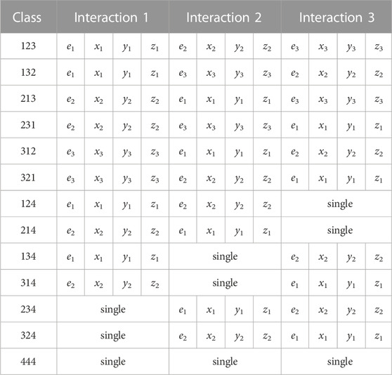
TABLE 1. The input class as the left column and the remaining columns contain the interaction data with subscripts for the correct interaction number. The top row indicates the order the interaction data will be fed into the neural network.

2.1.3 Standardization and normalization

In order to give our network a better chance at learning we change our data spread and distribution [21]. We use sklearn’s preprocessing objects for all normalization and standardization [22]. Additionally, we examined the importance of each variable doing a variable importance study, as described in Chapter 16 of [23], but all variables were shown to be of similar importance. Energy deposition is slightly more influential than Euclidean distance which is slightly more influential than individual coordinates (x₁, …, z₃). In this context “influential” means that a particular feature contributes more to correct classification than other features. It seems that all input features, including the computed ones, are of similar importance and removing any single feature would cause a direct drop in accuracy.

Our data and problems come from Compton camera detection issues related to interaction orderings. The fact that all of the interactions are randomly ordered means that like-columns such as energy or spatial coordinates are not strictly independent. If an energy value could be placed in e₁, e₂, or e₃, then treating these columns as separate and independent misrepresents what the columns mean. In order to properly address this, we standardize and normalize like-columns as a single feature but train on them as separate features. This is implemented by a reshaping, otherwise referred to as “wrap,” of the data such that we the x-, y-, z-coordinates of all interactions form one column each. This can be mathematically expressed as reshaping of a matrix $E\in {\mathbb{R}}^{n\times 3f}$ containing n events with three interactions and f features per interaction. For normalization, we reshape E such that it becomes $R\in {\mathbb{R}}^{3n\times f}$ and then normalize by column. To visualize this reshaping process, consider Figure 1, where we have $E\in {\mathbb{R}}^{2\times 9}$. We know that E has three features per interaction and that our new matrix R after reshaping will be $R\in {\mathbb{R}}^{6\times 3}$. We choose to mutate the spatial coordinates independently of the energy depositions. For the spatial coordinates we use the sklearn MaxAbsScaler to standardize them to the [−1, 1] range. Then we use the sklearn PowerTransformer with the Yeo-Johnson method to bring our energy deposition values closer to a normal distribution. These data manipulators are then saved using Python pickle for future usage.

FIGURE 1

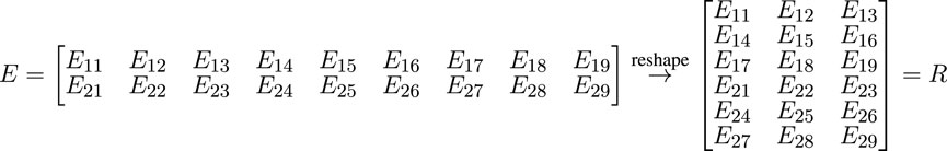
FIGURE 1. A demonstration of the data wrapping process performed by numpy.

After all of the data manipulation has been performed, we compute the Euclidean distance δ_ij for the ith and jth interaction. We append δ₁₂ to interaction 1, δ₂₃ to interaction 2, and δ₃₁ to interaction 3. Lastly we use pandas to save our data as a CSV.

2.2 Neural network construction and configuration

2.2.1 Fully connected residual blocks

The network used in the Results. is a deep fully connected neural network. Neural networks, especially fully connected ones, break down once they start becoming notably deep and complex. One of the first problems is that the values start to become very small during the forward propagation process. This leads to zeros and nearly zero values becoming more prominent as you go deeper and deeper. A partial fix to this forward propagation issue is to use Leaky ReLU (Rectified Linear Unit) over the traditional ReLU [24]. Another fix is data normalization between layers and before learning [25]. The second problem is that accuracy starts to degrade after a certain point in training despite no signs of training data memorization [25]. This phenomenon is discussed more intimately in [25] where they detail these effects. The major breakthrough solution to this problem is also proposed in [25] where they create ResNet, a network built from “residual blocks.” We use their original implementation of residual blocks as the basis for our fully connected residual blocks. Consider an arbitrary record. We pass it as an input to a small group of layers with their own activators. The result of the layer digestion is then concatenated with the original record. The concatenation in our case, and the case of the original ResNet, is addition. This addition operation helps, through the forward propagation process, keep input data to each block fresh.

The residual block method in [25] concatenates the data before the activation function is applied. The second version of ResNet, called ResNetV2, concatenates after the activation function. The original residual blocks were designed and implemented using convolutional layers in an image classification network. We create residual blocks using only fully connected layers with post-activation concatenation for the classification of prompt gamma events. The fully connected residual blocks allows us to create a thin, yet very deep residual fully connected neural network which avoids the aforementioned problems. Studies in [26] confirm that without this residual block structure our deep network will stop learning and its accuracy degrade.

A visual representation of our fully connected residual block can be seen as a Supplementary Image S2.

2.2.2 Network generation and training regime

First, we start by creating a JSON file which contains all of the values we wish to use for the creation of our neural network at run time. This allows us to set network wide hyperparameters like: layer dropout rate, the inter-layer activation function, number of layers, neurons per layer, layer regularization type, residual block size, input layer dimension, and output layer dimensions. This JSON file also contains data that allows us to change some hyperparameters associated with the training process like: learning rate or a learning rate function, epochs, batch size, and the percent of records to be used in validation.

The network configuration is loaded and fed to a Python function which takes in the entire JSON as a Python dictionary; this information is then used to generate a Keras Model object. The first layer of the model will always be a Keras input layer, and the final layer of the model is always a Keras softmax activation layer. We always have an output dimension of 13 which is the number of classes used during classification. The hidden layers of the model are always made of num_layers/block_size many residual blocks with block_size fully connected layers per block. The activation function between any fully connected layers, called inter-layer activation, is always leaky ReLU and there is no activation function between the concatenation step and the proceeding fully connected layer. The dropout rate for all fully connected layers is set to 45% and no dropout was used between the concatenation and the following fully connected layer. No additional forms of regularization are used. In our preliminary results, we saw that batch normalization provided no noticeable benefits leading to no usage of batch normalization during training.

After generating the network and loading in the data with pandas, we split the data into a 80% training set and 20% validation set. We do not carve out a testing set, instead we generate clinically accurate test data sets with our MCDE model whenever needed. For the training process itself we use the Keras Model.fit method which is given epochs, batch size, a training set, a validation set, a few callbacks, and some dynamic learning rate function from the JSON parameter file. Our callbacks were a learning rate scheduler, an epoch timer, the Keras ModelCheckpoint, and a Keras CSVLogger. We always used the Adam optimizer and categorical crossentropy loss while training. When Keras finished fitting the data we save the model using the Keras Model.save method.

For the learning rate we opted to use a non-adaptive non-constant learning rate scheduler. We use the Keras LearningRateScheduler callback to create our step scheduler which prescribes the learning rate t_i for epoch i with

$t_i=L\left(i\right)=\left\{\begin{array}{cc}10^{-3}\hfill & 1\le i\le \frac{p}{3},\hfill \\ 10^{-4}\hfill & \frac{p}{3}<i\le \frac{2p}{3},\hfill \\ 10^{-5}\hfill & \frac{2p}{3}<i\le \frac{5p}{6},\hfill \\ 10^{-6}\hfill & \frac{5p}{6}<i\le p,\hfill \end{array}\right.(1)$

where p denotes the total number of epochs used for training. We chose this simple learning rate scheduler over more complex schedulers because it is straight forward and showed positive results.

Any values which can be set and are not discussed here are left as their respective default values.

2.2.3 Postprocessing

To generate a confusion matrix, we load in our test data using pandas. We also load in our model using Keras. The data manipulators that were used to generate the training data are loaded using pickle. The test data is pushed through the data manipulators with wrapping in the same manner as the training data. From there we use the Keras Model.predict method to get the predicted classes from the neural network. Lastly, we feed the resulting predictions and true class information to sklearn’s confusion matrix routines to generate a confusion matrix.

To reconstruct the original proton beam, we first load in the data manipulators, the test data, and the trained model. From there we use the Keras Model.predict method to get the predicted classes from the neural network. Then we use numpy Array.argmax to determine which class is most likely for all events. This class data is then used for the cleaning process. All misordered triples are reordered to produce the correct ordering. All DtoTs have their falsely coupled single decoupled and their remaining double reordered. All false events are removed and all non-false events are saved.

Following the neural network data preprocessing we do image reconstruction. Image reconstruction was performed using the Kernel Weighted Back Projection (KWBP) algorithm, described by [18]. For this study, a full 3D image was reconstructed with KWBP using an 180 mm × 120 mm × 512 mm imaging space. This was processed into 60 separate two-dimensional slices (3 mm thick), with each slice image having 120 pixels × 512 pixels (1 mm² pixel size) in the YZ-plane. These PG images were reconstructed using all events with a calculated initial energy ranging from 2.0–4.5 MeV where the doubles-to-triples initial energy is taken to be the sum of the energy deposited in the remaining interactions, and the triples initial energy is determined using the gamma ray tracking method described by [27]. All images presented are 2D image slices in the YZ planes, extracted from the 3D dataset. The KWBP reconstructions were performed using an NVIDIA V100 GPU, with reconstruction times ranging from 1–5 s depending on the number of events used for the reconstruction.

We evaluate the quality of the images using the Contrast-to-Noise Ratio (CNR) metric. We compute CNR as

$C=\frac{\left|{\mu }_{\text{BP\hspace{0.17em}Region}}-{\mu }_{\text{noise}}\right|}{{\sigma }_{\text{noise}}},(2)$

where μ_{BP Region} is defined as the mean pixel value within the high intensity region of the image, μ_noise is the mean value of the image background noise, and σ_noise is the standard deviation of the background noise. We define the area for μ_{BP Region} as the rectangular region ranging from 27 mm to 36 mm along the height and 184 mm by 254 mm along the length of the image, that is, inside the portion of the beam with the highest intensity. To compute μ_noise and σ_noise we choose a region well outside the high intensity region and use the pixel values within the rectangular region from 0 mm to 60 mm along the height and from 394 mm to 512 mm along the width of the image. This captures a diverse collection of noise in the background without favoring a reconstruction which may have zero noise in a small region after the fall off but a lot of noise around the noiseless region.

2.3 Hardware and software used

The studies in this work use a distributed-memory cluster of compute nodes with large memory and connected by a high-performance InfiniBand network. The following specifies the details:

• 2018 GPU node: 1 GPU node containing four NVIDIA Tesla V100 GPUs (5,120 computational cores, 16 GB onboard memory) connected by NVLink and two 18-core Intel Skylake CPUs. The node has 384 GB of memory (12 × 32 GB DDR4 at 2666 MT/s).

• 2013 GPU nodes: 18 hybrid CPU/GPU nodes, each two NVIDIA K20 GPUs (2,496 computational cores, 5 GB onboard memory) and two 8-core Intel E5-2650v2 Ivy Bridge CPUs (2.6 GHz clock speed, 20 MB L3 cache, four memory channels). Each node has 64 GB of memory (8 × 8 GB DDR3). The nodes are connected by a QDR (quad-data rate) InfiniBand switch.

These nodes are contained in the cluster taki of the UMBC High Performance Computing Facility (http://hpcf.umbc.edu).

All studies and preprocessing using one or more of the following Python packages with the respective version:

• Python 3.7.6,

• Tensorflow 2.4.0 and the bundled Keras

• Numpy 1.18.1,

• Scipy 1.4.1,

• Scikit-Learn 0.23.dev0,

• Pandas 1.1.0.dev0+690.g690e382 (configured for icc 19.0.1.144 20181018),

3 Results

3.1 Neural network training and validation performance

Our initial studies in [28] showed that our general NN configuration is capable of identifying both true and false triple scatters. In this study, we have expanded the complexity of the network to now consist of 64 residual blocks with eight fully connected layers per block yielding a total of 512 hidden layers. Each layer had 256 neurons per layer, a 45% dropout rate, and used leaky ReLU activation. This more complex network, as shown in these results, is able to handle more complex triple scatter datasets, that include true and false events, as well as DotT and false triples. Similar to [28], all data used for training and validation are simulated and are produced by the MCDE model discussed in Section 2.1.1. We use an 80/20 training/validation data split as is suggested in [15] but since our data is entirely simulated this split is arbitrary and done for consistency with other research within the domain.

In Figure 2, we show the training and validation plots for our NN trained over 18,000 epochs using a learning rate scheduler that prescribes successive drops from 10^–3 to 10^–6. We see that the accuracy starts out very low with an initial accuracy of roughly 8%. For the next several thousand epochs the accuracy increases rapidly as the network overcomes the poor accuracy enforced by the dropout behavior. Just as the training and validation accuracy start to plateau, there is sudden spike in accuracy at 1,500 epochs as the learning rate is tightened from 10^–3 to 10^–4. At 10,652 epochs, there is a small jump in accuracy with a large reduction in the epoch-to-epoch accuracy range as the learning rate is tightened from 10^–4 to 10^–5. Lastly, there is a small jump in accuracy at 13,580 epochs as the learning rate is tightened for the final time from 10^–5 to 10^–6.

FIGURE 2

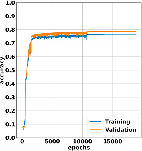
FIGURE 2. Training and validation plot for our NN over 18,000 epochs. The input data is divided into a training set and validation set which consist of 80% and 20% of the input data, respectively.

An interesting observation is that the validation accuracy is considerably higher than the training accuracy. This is most likely because Keras passes the training data through the network with dropout enabled but the validation data is passed through the network with dropout disabled. This allows the validation to be performed using all of the available neurons in the network as opposed to the reduced number of neurons used during training. The increased number of neurons present during validation most likely allows the network to perform better on validation data.

3.2 Prompt gamma event classification

Table 2 (a), 2 (b), 2 (c) are confusion matrices generated by our NN classifying the modeled 20,000 MU/min (Monitor Units per minute), 100 kMU/min, and 180 kMU/min dose rate data for the modeled 150 MeV beam, respectively. The first column (on the left side) of the confusion matrix is the input event class and the remaining columns are the percentages of the total respective input event class that is predicted to be the event class at the top of each column. Each cell is colored according to the maximum accuracy percentage (dark green) present in the entire confusion matrix.

TABLE 2

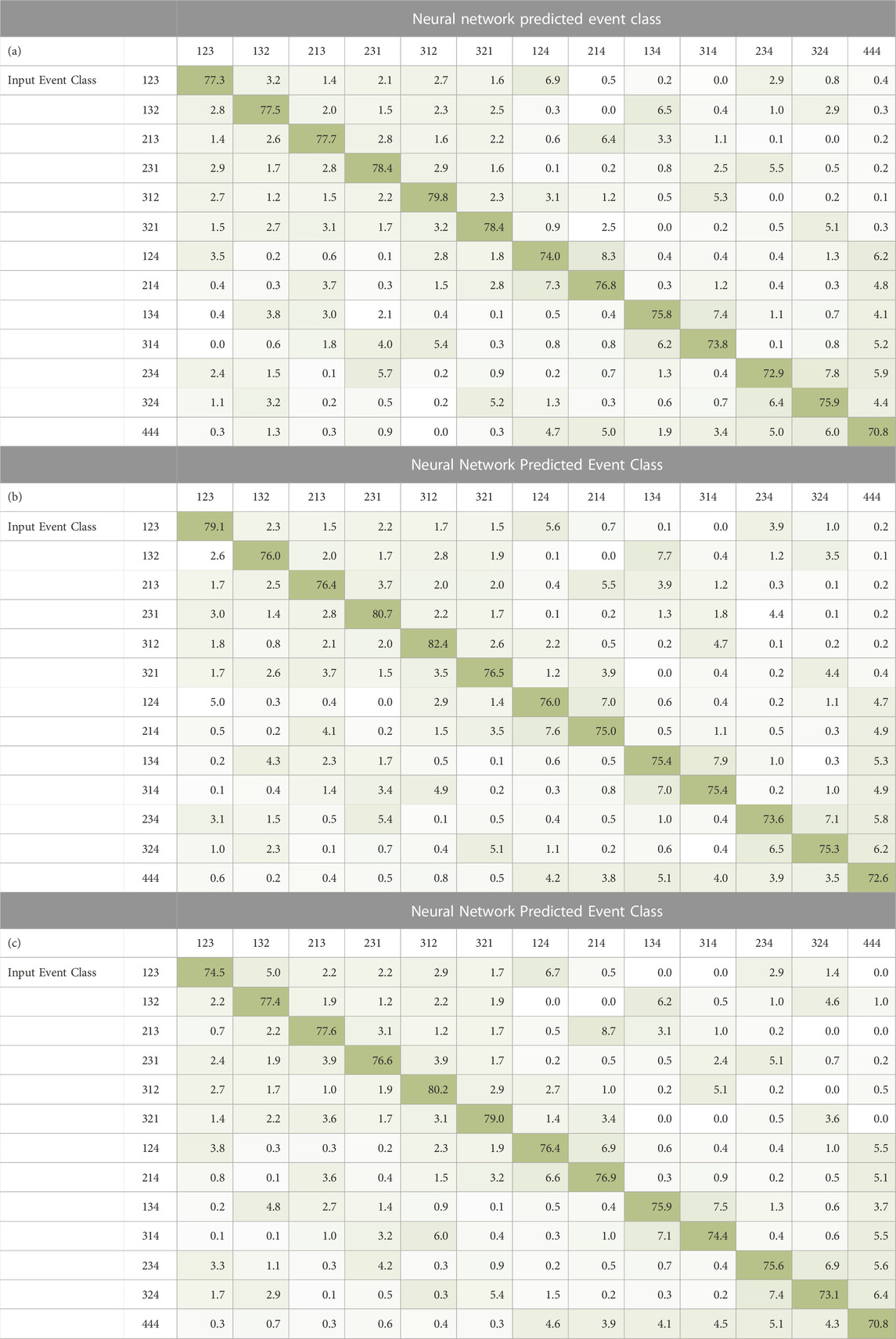
TABLE 2. Confusion matrix for a fully connected network trained on triples, double to triples, and false data from a 150 MeV beam for 18,000 epochs and tested on the MCDE model 150 MeV (a) 20 kMU/min, (b) 100 kMU/min, (c) 180 kMU/min beam. The 13 labels in the first column are the input event class and the remaining 13 columns are the percentages of the input which were predicted to be the event class at the top of column by the NN. Each cell is colored by accuracy relative to the largest percentage present in the entire confusion matrix.

We notice several general observations which hold for all confusion matrices in Table 2. We see that the dominant (highest percentage) event classification for each row is the input event class itself, indicating that the NN is correctly predicting the event type and ordering for a large percentage of all event classifications. The second highest prediction percentage for most classes of triple (classes 123, 132, 213, 231, 312, 321) are the DtoT classes with the same interaction ordering. This means that the network correctly identifies the first two interactions the best and, at times, struggles to correctly identify whether the third interaction truly belongs in the triple or not.

For the six DtoT classes (124, 214, 134, 314, 234, 324) we see that the second highest classification result for each DtoT event is actually a reverse ordering of the true double ordering. The NN can determine which of the three interactions does not belong to the true double scatter event but, after doing so, is unsure of the ordering two interactions. The third most likely network prediction for several DtoT classes is as a true triple. The two true interactions (of the DtoT’s true double) are correctly ordered, but the third interaction, an improperly coupled single, is incorrectly identified as the third interaction of the true triple. This improper identification of these DtoTs as valid triples creates events that would produce noise in the reconstructed image. The other DtoTs have false events as their third highest predicted class which is considered data loss but poses no detriment to reconstruction.

Any improper classification of false data as a true event means that we are increasing noise in our final reconstructed images. The dominant NN prediction for the false event class is also the false event class which is the preferred outcome. Most of the incorrect classifications for the false data is into the six DtoT classes which means that false doubles will be produced when one of the interactions is predicted to be an incorrectly coupled single scatter and removed. Lastly, very few false events are incorrectly identified as a true triples class by the NN. This indicates that the network can easily distinguish between true and false events.

3.3 Prompt gamma image analysis based on neural network classification

To illustrate the effect that network event classification can have on the PG images produced from the camera data, reconstructed PG images are shown in Figure 3 along with the ground truth images of the proton dose deposition. In Figure 3, there are four rows of PG image reconstructions. In the first row we see the actual dose deposition by the proton beam, showing the characteristic Bragg peak at the end of its range (near the center of the image). This is because the Bragg peak is considered to be the ground truth or “best case scenario” for PG image reconstruction. The remaining three rows in Figure 3 are reconstructions of three PG data recorded by the camera for proton beam irradiation at clinical dose rates of 20 kMU/min, 100 kMU/min, and 180 kMU/min. The images in the left column are the respective PG images reconstructed with raw data prior to NN classification, otherwise called the “uncleaned” data. The images in the right column are the respective PG images reconstructed with data after it has been corrected based on the NN classifications, otherwise called the “cleaned” data. Since each PG image is from data collected during delivery of the same 150 MeV proton beam they will have the same position and range even though they are reconstructed from data collected at different dose rates.

FIGURE 3

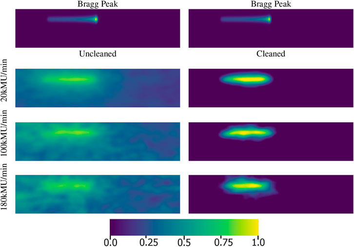
FIGURE 3. The first row contains a reconstruction of the proton beam with a Bragg peak at the end of its range. The second, third, and fourth rows are reconstructions of PG data recorded at 20 kMu/min, 100 kMU/min, and 180 kMU/min dose rates, respectively. The left column uses PG data without using the NN classification for data correction, called the “uncleaned” data. The right column uses PG data after it has been NN classified and corrected, called the “cleaned” data. Each image is 120 by 512 pixels and each pixel represents a 1 mm² area. The images are normalized such that pixels with no energy depositions are the darkest with a value of 0.0 and the pixels with the maximum energy deposition are the brightest with a value of 1.0.

When we evaluate the uncleaned and cleaned data it is clear that as the beam dose rate increases we get a decrease in visual quality for the PG images, with a reduced image signal with respect to the image background. This loss of image contrast can be seen in image CNR (Contrast-to-Noise Ratio) of 33, 23, and 10 for the uncleaned data images at 20 kMU/min, 100 kMU/min, and 180 kMU/min, respectively. However, when the data is classified by the NN and corrected, the CNR values improve to 41, 30, and 22 for the cleaned data 20 kMU/min, 100 kMU/min, and 180 kMU/min, respectively. The improved values in the cleaned data correlate well to the improved visual appearance of the beam in which the start point and end point are now easily distinguishable at all three dose rates.

4 Discussion

We use a deep residual fully connected NN to determine the proper ordering and coupling behavior of Compton camera data. In many classification problems, misclassifications are seen as a complete loss with no benefits, but for our problem this is not entirely true. Consider the fact that for our imaging problems we are limited by the number of PGs that camera can measure during the delivery of a single proton therapy treatment session. For this reason, any opportunity that data can be recovered must be seized, since it is not possible to deliver more doses to a patient again if more data are needed.

Consider the case of a triple classified as DtoT where the single scatter interaction is thrown away and the interactions of the recovered true double are correctly ordered. This produces a valid true double which can still be used for reconstruction. For instance, in Table 2 (c), the 213 class has a classification accuracy of 77.6%. This would normally imply that we have lost 22.4% of the remaining 213 events. However, when a 213 is classified as a 214, we still have a valid double. From Table 2 (c), we see that the 213 class was misclassified as a 214 with 8.7% of the time. This means that given a misordered 213 true triple, which is unusable for reconstruction, we recover 86.3% of the input class and convert it into a correctly ordered true triple or true double which are then usable for reconstruction. When a DtoT is classified as a false triple, this is a beneficial situation as we know that it will be removed from the data so it cannot cause noise in the reconstructed image. As for DtoTs which are misordered, if the true double that is part of the DtoT is properly identified, it is possible to pass it to a separate doubles classification network so its order may still be corrected as described in [19].

The addition of false triple classification to true triple and DtoT classification required significantly more configuration and training time. We believe this is because false triples are similar to DtoTs, in that they both contain falsely coupled single scatters. We believe similarities between these event classes leads the network to misclassify false triples as DtoT events. This could be problematic since the false triples which are classified as DtoTs would be converted to a (false) double which would produce noise in the image if used for reconstruction. In principle if passed to a doubles classification network, it could be identified as a false double and removed.

From here it is important to discuss how the NN is improving the data in a literal sense. Our confusion matrices demonstrate how the NN performs on each class in isolation, but they do not illustrate how the NN changes the balance of the data files. The data produced by the Compton camera, in the context of classes, is unbalanced and largely dependent on the dose rate. As the dose rate increases from a clinical minimum of 20 kMU/min to a clinical maximum of 180 kMU/min as outlined in [29], the number of true triples decreases while the number of DtoTs and false triples increases. At 180 kMU/min most of the data being detected is almost entirely DtoT and false triples. Table 3 shows percentages, compiled from the presented confusion matrices, of the measured PG data that would be usable for image reconstruction before and after NN event classification. For instance, if 100,000 triple events have been measured with our Compton camera, at 180 kMU/min dose rate, around 5,600 true triples would be measured [29]. If we assume each of the six possible interaction orderings are equally possible, then only 936 are correctly ordered meaning only 0.9% of all of the detected events can be used for reconstruction. If we were to use our NN for classifying and correcting the event ordering, based on the percentages in Table 2 (c), then around 4,356 of the 5,600 true triples will be usable for reconstruction. The remaining 94.4% of the measured events are DtoTs and false triples [29]. Without the NN these events are passed directly to the reconstruction process and produce noise in the reconstructed images. After using the NN classification, 34,692 false triples would be removed and 34,544 DtoTs are recovered as true properly ordered doubles (and used for reconstruction). Before we used the NN, only 0.9% of the data passed to the reconstruction method is actually viable for reconstruction; after we use the NN and remove false events, recover true doubles from DtoTs, and correctly order the interactions in all true events, 59.6% of the remaining data is now viable for reconstruction, an improvement of 58.7%. At the lower dose rates we see even larger gains with 20 kMU/min going from 7.9% usable events to 78.0% usable events, an improvement of 70.1%, and 100 kMU/min going from 1.8% usable event to 73.8% usable events, an improvement of 72.0%.

TABLE 3

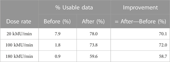
TABLE 3. Given 100,000 PG scatterings detected by the Compton camera and the rate of Compton camera event misdetection, what percentage of the detected data is usable for PG image reconstruction before and after using the NN for event correction at varying dose rates.

The effect that the improved data quantity and quality has on image reconstruction can be seen visually in Figure 3. The large image background seen in the uncleaned data images is almost completely removed by the NN classification and data correction as can be seen in the cleaned data images. More detailed results and discussions about the impact of NN processing on the use and viability of CC based imaging in clinical proton radiotherapy are the focus of [30]. For example, in [30] it was shown that the neural network has a noticeably significant improvement in the before/after energy spectra.

Lastly, it important to touch upon the possibility of integrating a neural network into a real-time detection scenario. Let us consider an “end-to-end solutions” as one where: the Compton camera detects the prompt gammas, whereby the data is handled and digested by some routines, this is then passed to the neural network for classification and cleaning, that result is then reconstructed, and then that result is available to the party requiring it via some display. When discussing this topic, with this definition, keep in mind that there are many things which can impact the performance of an end-to-end solution beyond the neural network. Since our definition is very loose and there is no formal end-to-end solutions in practice that can be used for comparison, instead we ask the question: will a neural network inhibit or bottleneck the performance of a developed solution? The neural network itself can process millions of events in under a second and clean the data in under a second. Additionally, our neural network could most likely be simplified to improve cleaning speed even more. If we assume that feedback is required within 5 s of a dose, then this leaves roughly 3–4 s for the remaining aspects of the pipeline depending on the number of events detected. It is more likely that some of component of the end-to-end pipeline will need to be addressed for the speed of classification and cleaning comes into question.

Our results here are a demonstration that neural networks can serve as an important piece to the Compton camera prompt gamma reconstruction pipeline to help improve the quality of the results obtained from image reconstruction. For future work a full range of proton energies will need to be studied, 70 MeV–250 MeV, with a multitude of network architectures and configurations to test complete viability. It is likely that the patterns embedded within the scattering data does not change as the energies change, something which is independent of the distribution of the scatter classes, though the values themselves may differ highly. This motivates research into additional, and perhaps more novel, data preprocessing methods which help smooth out the irrelevant differences between the varying energy levels.

Data availability statement

The raw data supporting the conclusion of this article will be made available by the authors, without undue reservation.

Author contributions

JP conceived the approach to the problem. JP generated all of the initial data for reconstruction and performed the reconstruction of the cleaned data. CB created, trained, validated, and tested the neural network. CB, MG, JP designed the event selection routine. CB and JP analyzed the resulting data. CB, MG, and JP wrote the manuscript, which was reviewed and approved by all authors.

Funding

This work is supported by the grant “CyberTraining: DSE: Cross-Training of Researchers in Computing, Applied Mathematics and Atmospheric Sciences using Advanced Cyberinfrastructure Resources” from the National Science Foundation (grant no. OAC–1730250). This work is also supported by the grant “REU Site: Online Interdisciplinary Big Data Analytics in Science and Engineering” from the National Science Foundation (grant no. OAC–2050943). The research reported in this publication was also supported by the National Institutes of Health National Cancer Institute (grant no. R01CA187416). The content is solely the responsibility of the authors and does not necessarily represent the official views of the National Institutes of Health. The hardware used in the computational studies is part of the UMBC High Performance Computing Facility (HPCF). The facility is supported by the United States National Science Foundation through the MRI program (grant nos. CNS–0821258, CNS–1228778, OAC–1726023, CNS–1920079) and the SCREMS program (grant no. DMS–0821311), with additional substantial support from the University of Maryland, Baltimore County (UMBC). See http://hpcf.umbc.edu for more information on HPCF and the projects using its resources.

Conflict of interest

The authors declare that the research was conducted in the absence of any commercial or financial relationships that could be construed as a potential conflict of interest.

Publisher’s note

All claims expressed in this article are solely those of the authors and do not necessarily represent those of their affiliated organizations, or those of the publisher, the editors and the reviewers. Any product that may be evaluated in this article, or claim that may be made by its manufacturer, is not guaranteed or endorsed by the publisher.

Supplementary material

The Supplementary Material for this article can be found online at: https://www.frontiersin.org/articles/10.3389/fphy.2023.903929/full#supplementary-material

References

1. Wilson RR. Radiological use of fast protons. Radiology (1946) 47:487–91. doi:10.1148/47.5.487

PubMed Abstract | CrossRef Full Text | Google Scholar

2. Bragg WH, Kleeman R. On the ionization curves of radium. Lond Edinb Dublin Philos. Mag. J. Sci. (1904) 8:726–38. doi:10.1080/14786440409463246

CrossRef Full Text | Google Scholar

3. Polf JC, Parodi K. Imaging particle beams for cancer treatment. Phys Today (2015) 68:28–33. doi:10.1063/PT.3.2945

CrossRef Full Text | Google Scholar

4. Fontana M, Ley J, Dauvergne D, Freud N, Krimmer J, Létang JM, et al. Monitoring ion beam therapy with a Compton camera: Simulation studies of the clinical feasibility. IEEE Trans Radiat Plasma Med Sci (2020) 4:218–32. doi:10.1109/TRPMS.2019.2933985

CrossRef Full Text | Google Scholar

5. Rohling H, Priegnitz M, Schoene S, Schumann A, Enghardt W, Hueso-González F, et al. Requirements for a Compton camera for in vivo range verifications of proton therapy. Phys Med Biol (2017) 62:2795–811. doi:10.1088/1361-6560/aa6068

PubMed Abstract | CrossRef Full Text | Google Scholar

6. Krimmer J, Dauvergne D, Létang JM, Testa É. Prompt-gamma monitoring in hadrontherapy: A review. Nucl Instr Methods Phys Res A (2018) 878:58–73. doi:10.1016/j.nima.2017.07.063

CrossRef Full Text | Google Scholar

7. Compton AH. A quantum theory of the scattering of x-rays by light elements. Phys Rev (1923) 21:483–502. doi:10.1103/PHYSREV.21.483

CrossRef Full Text | Google Scholar

8. Schönfelder V, Hirner A, Scheider K. A telescope for soft gamma ray astronomy. Nucl Instr Meth. (1973) 107:385–94. doi:10.1016/0029-554X(73)90257-7

CrossRef Full Text | Google Scholar

9. Todd RW, Nightingale JM, Everett DB. A proposed γ camera. Nature (1974) 251:132–4. doi:10.1038/251132a0

CrossRef Full Text | Google Scholar

10. Maggi P, Peterson S, Panthi R, Mackin D, Yang H, He Z, et al. Computational model for detector timing effects in Compton-camera based prompt-gamma imaging for proton radiotherapy. Phys Med Biol (2020) 65:125004. doi:10.1088/1361-6560/ab8bf0

PubMed Abstract | CrossRef Full Text | Google Scholar

11. Oberlack UG, Aprile E, Curioni A, Egorov V, Giboni KL. Compton scattering sequence reconstruction algorithm for the liquid xenon gamma-ray imaging telescope (lxegrit). In: Hard X-ray, gamma-ray, and neutron detector physics II (2000). doi:10.1117/12.407578

CrossRef Full Text | Google Scholar

12. Boggs SE, Jean P. Event reconstruction in high resolution compton telescopes. Astron Astrophys Suppl Ser (2000) 145:311–21. doi:10.1051/aas:2000107

CrossRef Full Text | Google Scholar

13. Zoglauer A, Boggs SE. Application of neural networks to the identification of the Compton interaction sequence in Compton imagers. In: IEEE Nuclear Science Symposium Conference Record, Honolulu, HI, (2007). doi:10.1109/NSSMIC.2007.4437096

CrossRef Full Text | Google Scholar

14. Barajas CA, Kroiz GC, Gobbert MK, Polf JC. Classification of Compton camera based prompt gamma imaging for proton radiotherapy by random forests. In: The 2021 International Conference on Computational Science and Computational Intelligence (CSCI 2021), Las Vegas, NV, (2021), 308–311. (in press).

CrossRef Full Text | Google Scholar

15. Chollet F. Deep Learning with Python. Shelter Island, NY: Manning Publications Co. (2018).

Google Scholar

16. Muñoz E, Ros A, Borja-Lloret M, Barrio J, Dendooven P, Oliver JF, et al. Proton range verification with MACACO II Compton camera enhanced by a neural network for event selection. Sci Rep (2021) 11:9325. doi:10.1038/s41598-021-88812-5

PubMed Abstract | CrossRef Full Text | Google Scholar

17. Takashima S, Odaka H, Yoneda H, Ichinohe Y, Bamba A, Aramaki T, et al. Event reconstruction of Compton telescopes using a multi-task neural network. Nucl Instr Methods Phys Res Section A: Acc Spectrometers, Detectors Associated Equip (2022) 1038:166897. doi:10.1016/j.nima.2022.166897

CrossRef Full Text | Google Scholar

18. Panthi R, Maggi P, Peterson S, Mackin D, Polf J, Beddar S. Secondary particle interactions in a Compton camera designed for in vivo range verification of proton therapy. IEEE Trans Radiat Plasma Med Sci (2021) 5:383–91. doi:10.1109/TRPMS.2020.3030166

PubMed Abstract | CrossRef Full Text | Google Scholar

19. Kroiz GC, Barajas CA, Gobbert MK, Polf JC. Exploring deep learning to improve Compton camera based prompt gamma image reconstruction for proton radiotherapy. In: The 17th International Conference on Data Science (ICDATA’21), Las Vegas, NV, (2021). (accepted).

Google Scholar

20. Agostinelli S, Allison J, Amako K, Apostolakis J, Araujo H, Arce P, et al. Geant4–a simulation toolkit. Nucl Instr Methods Phys Res Section A: Acc Spectrometers, Detectors Associated Equipment (2003) 506:250–303. doi:10.1016/S0168-9002(03)01368-8

CrossRef Full Text | Google Scholar

21. LeCun YA, Bottou L, Orr GB, Müller KR. Efficient BackProp. Berlin, Heidelberg: Springer Berlin Heidelberg (2012). p. 9–48. doi:10.1007/978-3-642-35289-8_3

CrossRef Full Text | Google Scholar

22. Pedregosa F, Varoquaux G, Gramfort A, Michel V, Thirion B, Grisel O, et al. Scikit-learn: Machine learning in Python. J Mach Learn Res (2011) 12:2825–30.

Google Scholar

23. Biecek P, Burzykowski T. Explanatory model analysis. New York: Chapman and Hall/CRC (2021).

Google Scholar

24. Maas AL, Hannun AY, Ng AY. Rectifier nonlinearities improve neural network acoustic models. In: ICML Workshop on Deep Learning for Audio, Speech and Language Processing, Atlanta, GA, (2013).

Google Scholar

25. He K, Zhang X, Ren S, Sun J. Deep residual learning for image recognition. In: 2016 IEEE Conference on Computer Vision and Pattern Recognition (CVPR), Las Vegas, NV, (2016). p. 770–8. doi:10.1109/CVPR.2016.90

CrossRef Full Text | Google Scholar

26. Barajas CA, Kroiz GC, Gobbert MK, Polf JC. Deep learning based classification methods of Compton camera based prompt gamma imaging for proton radiotherapy. Tech. Rep. HPCF–2021–1. In: UMBC High Performance Computing Facility. Baltimore: University of Maryland, Baltimore County (2021).

Google Scholar

27. Schmid G, Deleplanque M, Lee I, Stephens F, Vetter K, Clark R, et al. A γ-ray tracking algorithm for the greta spectrometer. Nucl Instr Methods Phys Res Section A: Acc Spectrometers, Detectors Associated Equip (1999) 430:69–83. doi:10.1016/S0168-9002(99)00188-6

CrossRef Full Text | Google Scholar

28. Barajas CA, Kroiz GC, Gobbert MK, Polf JC. Using deep learning to enhance Compton camera based prompt gamma image reconstruction data for proton radiotherapy. Proc Appl Math Mech (PAMM) (2021) 21:e202100236. doi:10.1002/pamm.202100236

CrossRef Full Text | Google Scholar

29. Polf JC, Maggi P, Panthi R, Peterson S, Mackin D, Beddar S. The effects of Compton camera data acquisition and readout timing on PG imaging for proton range verification. IEEE Trans Radiat Plasma Med Sci (2021) 6:366–73. doi:10.1109/TRPMS.2021.3057341

PubMed Abstract | CrossRef Full Text | Google Scholar

30. Polf JC, Barajas CA, Peterson SW, Mackin DS, Beddar S, Ren L, et al. Applications of machine learning to improve the clinical viability of Compton camera based in vivo range verification in proton radiotherapy. Front Phys (2022) 10:838273. doi:10.3389/fphy.2022.838273

PubMed Abstract | CrossRef Full Text | Google Scholar