 Hongli Guan1,2,3,4
 Wang Zhao1,2,3Shuai Wang1,2,3*Kangjian Yang1,2,3Mengmeng Zhao1,2,3Shenghu Liu1,2,3,4Han Guo1,2,3Ping Yang1,2,3*
- 1National Key Laboratory of Optical Field Manipulation Science and Technology, Chinese Academy of Sciences, Chengdu, China
- 2Key Laboratory on Adaptive Optics, Chinese Academy of Sciences, Chengdu, Sichuan, China
- 3Institute of Optics and Electronics, Chinese Academy of Sciences, Chengdu, Sichuan, China
- 4School of Optoelectronics, University of Chinese Academy of Sciences, Beijing, China
The limited spatial sampling rates of conventional Shack–Hartmann wavefront sensors (SHWFSs) make them unable to sense higher-order wavefront distortion. In this study, by etching a known phase on each microlens to modulate sub-wavefront, we propose a higher-resolution wavefront reconstruction method that employs a modified modal Zernike wavefront reconstruction algorithm, in which the reconstruction matrix contains quadratic information that is extracted using a neural network. We validate this method through simulations, and the results show that once the network has been trained, for various atmospheric conditions and spatial sampling rates, the proposed method enables fast and accurate high-resolution wavefront reconstruction. Furthermore, it has highly competitive advantages such as fast dataset generation, simple network structure, and short prediction time.
1 Introduction
A Shack–Hartmann wavefront sensor (SHWFS) is developed based on the classical Hartmann wavefront measurement method, with the advantages of simple installation, compact structure, reliable algorithm, and fast measurement speed [1]. It has been widely used in astronomical observation [2], biomedical imaging [3, 4], high-energy laser beam quality testing [5], space communication systems [6], and optical tweezers [7]. In principle, SHWFS utilizes the microlens array (MLA) to sample the incident wavefront to produce a spot array pattern, computes the relative offset of the spot centroid, and then reconstructs the wavefront using the algorithm. In this process, the sub-wavefront is regarded as a plane wave.
According to the principle of SHWFS, it detects high spatial frequency wavefronts and demands MLA with enough spatial sampling rates. However, when the source is faint, very high spatial sampling rates not only reduce the spot intensity but also decrease the stability and accuracy of the reconstruction. [8, 9] used MLA with lower spatial sampling rates, which caused the spatial resolution of the SHWFS to decrease. In recent years, a series of improvement methods have been proposed to improve the measurement performance of SHWFS at a low spatial sampling rate. Meimon et al. added a known astigmatism to the sub-wavefront and proposed the linearized focal-plane technique (LIFT) phase retrieval method, which can sense more modes with fewer subapertures [10, 11]. Li et al. placed a detector at a defocus plane of MLA and reconstructed the incident wavefront using the intensity distribution information of spots. This method can sense higher-order aberrations [12]. Zhao et al. introduced four-quadrant binary phase modulation into each subaperture and used an optimization algorithm to reconstruct the wavefronts with high accuracy [13]. Zhu et al., based on LIFT, proposed the focal technique to sense more Zernike modes in each subaperture and optimized the relative parameters. The simulations and experiments proved that the method can accurately reconstruct the wavefront [14]. Feng et al. used the first and second moments to express information of the sub-wavefront and reconstructed high-frequency aberration of the incident wavefront [15]. Wu et al. proposed using multiple low-sampling-rate SHWFS to achieve high-resolution wavefront sensing and applied this technique to extended objects [16]. All of the above studies have offered new approaches, and yet, for timeliness, sensitivity, stability, and simplicity of detection, these approaches do not entirely take them into account. Fortunately, we find that machine learning can accomplish this work excellently.
Machine learning, a popular current research approach with short computational time and excellent nonlinear fitting ability, has been proven to be an effective alternative to the standard modal Zernike wavefront reconstruction algorithm (hereafter referred to as the traditional method). In the past few years, for low spatial sampling rate studies, several methods based on machine learning have also been proposed. Xu et al. used an extreme learning machine to fit the nonlinear corresponding relationship between the centroid displacement and Zernike coefficients. Under sparse microlens, the reconstruction result of the method is much more accurate than that of the standard traditional method [17]. He et al. proposed using ResNet to restore Zernike coefficients directly from sparse subaperture spot images instead of the whole spot array pattern. The method broke the limitation of d/r0 = 1 (where d is the length of the subaperture and r0 is the coherence diameter) and used transfer learning to reduce the training time [18]. The deep-phase retrieval wavefront reconstruction method was proposed by Guo et al.; this method realized high-speed and high-spatial-resolution wavefront measurement [19]. However, when confronted with different spatial sampling rates, these methods become impotent.
In this paper, we treat the sub-wavefront as a quadratic surface instead of a simple plane. On the basis of the new assumption, a method of high-resolution wavefront reconstruction based on sub-wavefront information extraction is proposed, which includes two parts:
1. All full-light sub-spots are considered to have consistent features, and their slope and quadratic information are extracted using a neural network. This approach enables quick dataset generation, employs a simple network, and reduces prediction time. In addition, the trained network can predict sub-wavefront information with different sampling rates.
2. Modifying the traditional method by adding quadratic information to the reconstruction matrix, the wavefront may be reconstructed quickly and accurately.
Compared with the traditional method, the proposed method can reconstruct the wavefront with higher spatial resolution, or the same spatial resolution reconstruction can be accomplished with a lower sampling rate, providing a new way for high-resolution wavefront detection and faint source wavefront detection.
The remainder of the article is organized as follows: Section 2 establishes a new sub-wavefront assumption, introduces the method of extracting sub-wavefront information, and modifies the wavefront reconstruction algorithms. Section 3 presents the simulation model, the results of the training network, and the reconstruction wavefront result. In Section 4, the fitting error of the sub-wavefront and the spatial resolution of the proposed algorithm are discussed. In addition, we analyze the factors that affect spatial resolution. Finally, Section 5 presents the conclusion drawn from the research.
2 Methods
2.1 Sub-wavefront assumption
In the process of SHWFS detection, MLA samples the incident wavefront, with amplitude and phase information fully presented in the spot array pattern. In other words, SHWFS has detected all the information of the wavefront, and the optical structure of SHWFS does not constrain the spatial resolution reconstruction. The limitation on the spatial resolution arises from its assumption (Eq. 1), where each sub-wavefront is approximately regarded as a tip-and-tilt plane.
where c1 and c2 are wavefront slope information and ε is the fitting error.
Therefore, the wavefront reconstruction algorithms of SHWFS are based on the plane assumption, which ignores the high-order information of the sub-wavefront. If the assumption is changed as expressed in Eq. 2, i.e., using a quadratic surface to fit, this can more accurately express the sub-wavefront.
Here, the quadratic information is represented by c3, c4, and c5 and ε’ is the fitting error.
The result of using the two assumptions to fit a random sub-wavefront is shown in Figure 1. Figure 1A shows a sub-wavefront, and Figures 1B, C represent the fitting errors of the two assumptions, respectively. The root mean square (RMS) value and the peak valley (PV) value are shown in the figure, which can intuitively illustrate the virtue of the novel assumption. By extracting the slope and quadratic information of the sub-wavefront (both are called sub-wavefront information), it is expected to reach high spatial resolution measurement.
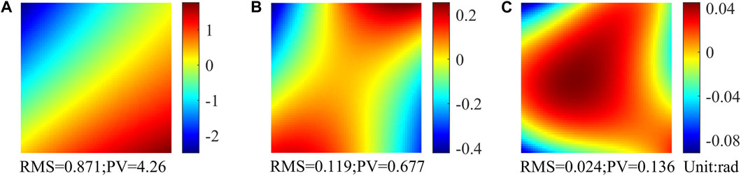
FIGURE 1. (A) Sub-wavefront; (B) error of plane fitting; and (C) error of quadratic surface fitting.
2.2 Extracting sub-wavefront information
2.2.1 Modulating sub-wavefront
Obtaining sub-wavefront information solely from the centroid offset is challenging; to complete this work, we need to use the intensity distribution information within the spot. However, same as the phase retrieval (PR) algorithm [20], which is based on the spot intensity distribution, there is a multiple-solution problem. Referring to the article [13] to solve the problem, in this paper, the sub-wavefront is modulated by a four-quadrant binary phase whose expression is given by Eq. 3.
where x∈[−d1/2, d1/2], y∈[−d2/2, d2/2], and d1 and d2 are the length and width of the phase modulation area; in this paper, the area corresponds to a subaperture range.
As shown in Figure 2, by rotating the wavefront Φ1 (x,y) 180° and flipping it, the new wavefront Φ2 (x,y) = -Φ1 (−x,−y) can be acquired. With four-quadrant binary phase modulation, a pair of rotating and flipping wavefronts (Φ1 and Φ2) will not have the same spot. Thus, the multiple-solution problem can be avoided by performing the phase on a sub-wavefront. This only requires etching a four-quadrant binary phase on each microlens surface, and the main structure of SHWFS does not change. As such, it is feasible to utilize neural networks to predict the sub-wavefront information based on the spot.
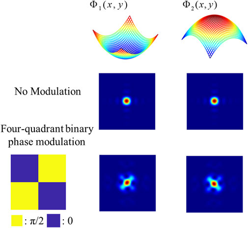
FIGURE 2. Far-field spot of non-modulation and phase modulation.
2.2.2 Neural network extracts sub-wavefront information
In this paper, the sub-wavefront information is extracted by a neural network, whose structure is shown in Figure 3. Using a modulated spot pattern as an input to the network, different sizes of feature patterns can be obtained by handling different convolutional layers (with 1 × 1, 2 × 2, 3 × 3, and 4 × 4 kernel sizes and 4, 8, 12, and 16 depths, respectively) in parallel and fusing these feature maps via a depth concatenation layer. Aiming to keep the detailed information, a convolutional layer (with a 3 × 3 kernel size and 40 depths) replaces the pooling layer. Then, a 31 × 31 × 40 feature map is taken as an input for the next layer. Once again, a 16 × 16 × 120 feature map is obtained. After each convolutional layer, an activation function (ReLU function) is added to reduce the training time and fit the nonlinear relationship between the input and output. Finally, it passes through the fully connected layers with 256, 64, and 5 neurons, respectively. The fully connected layer outputs five parameters, representing the information of a sub-wavefront.
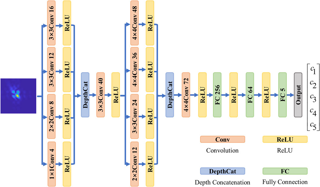
FIGURE 3. Structure of a neural network.
The dataset generation process is shown in Figure 4. The input wavefront is split into several sub-wavefronts by MLA, simultaneously forming a spot array pattern. This process satisfies the angular spectrum transport theory [21]. In the spot array pattern, which includes information of the incident wavefront, each spot similarly contains the corresponding sub-wavefront information. If the effects of imaging between spots are ignored, the formation of a spot can be considered an independent imaging process. Moreover, the input wavefront satisfies an atmospheric turbulence model (e.g., the Kolmogorov model), which implies that the spot patterns have the same characteristic distribution. Thus, a spot pattern is segmented from the spot array pattern, and together with the corresponding sub-wavefront information, a dataset can be generated.

FIGURE 4. Dataset generation process.
Furthermore, as long as the incident wavefront has the same atmospheric parameters (for example, d/r0 = 1), it is able to produce datasets with the same characteristic distribution, even if the sampling rates are different. Obviously, an incident wavefront can produce more than one dataset, and the data volume of a spot is much smaller than the entire spot map, which means that it is able to generate datasets and train networks quickly. Furthermore, the network has a short prediction time and can be used to extract sub-wavefront information with different sampling rates.
The incident wavefront Φ can be expressed using Zernike polynomials as follows:
where Zk represents the kth-order Zernike polynomial, ak is the coefficient of Zk, and p is the number of Zernike modes.
The ith sub-wavefront Φsub can be represented by Eq. 2, and the relationship between the sub-wavefront information and the Zernike coefficient is
where Si is the normalized subaperture area.
It is worth noting that only full-light spots can be regarded as having uniform features; therefore, only full-light sub-wavefront information can be extracted using this method. For non-full-light subaperture, the relationship between the sub-wavefront slope information and Zernike coefficients is as follows:
We can only obtain slope information from the center of gravity (COG), but all of this correct information is valuable for wavefront reconstruction.
2.3 Wavefront reconstruction algorithm
Under the new sub-wavefront assumption, it is critical to reconstruct the incident wavefront with all the extracted information. Referring to the traditional method, taking the quadratic information into the reconstruction matrix is the simplest method. In the event that the SHWFSs have n non-full-light subapertures and m full-light subapertures, for P-order Zernike polynomials, the set of Eqs 4, 5 can be formulated into a matrix form as
The simple matrix formula is
In the process of wavefront detection, only A is unknown. Eq. 8 can be transformed into
where Z+ is the generalized inverse of Z. The common methods to calculate it are Gram–Schmidt orthogonalization [22] and singular value decomposition [23].
3 Simulation
3.1 Network training
3.1.1 Simulation setup
To validate that the built neural network can predict sub-wavefront information, the process has been numerically simulated using MATLAB. The simulation setup is shown in Figures 5A, B. The match relationship between MLA and the optical pupil is shown in Figure 5B; the red region is the full-light subaperture, and the gray region is the non-full-light subaperture. This arrangement is used to obtain more full-light subapertures, which can reconstruct wavefronts more accurately with more information. In the simulation, we only considered monochromatic light and ignored the non-uniformity of the light intensity. Meanwhile, in the simulation, we introduced the noise of the camera that satisfies a normal distribution.
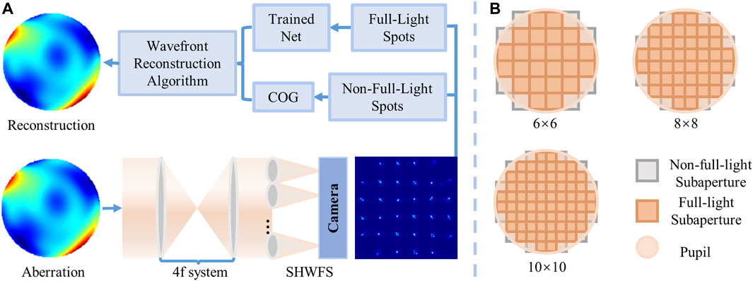
FIGURE 5. (A) Simulation setup of wavefront measurement; (B) matching relationship between pupil and subaperture.
The key parameters of the simulation are shown in Table 1. To better balance the robustness and prediction accuracy of the network, 71,280 datasets are generated from 3,510 random atmospheric wavefronts, with 10% of these randomly selected as test datasets. The atmospheric parameter is set to d/r0 = 1–3. For different sampling rates of the incident wavefront, this atmospheric parameter should also be maintained to produce datasets with consistent features.

TABLE 1. Key parameters of the simulation.
Furthermore, for optimizing the weights of the network, an adaptive moment estimation (Adam) optimizer is used, the initial learning rate is 0.001, and the epoch and batch size are set to 200 and 128, respectively. The training is performed on a desktop workstation (11th Gen Intel (R) Core (TM) i7-11700K @ 3.60GHz, RAM 16G, NVIDIA RTX3090 Ti).
3.1.2 Results of the trained network
In the training process, the loss function is the root mean square error (RMSE) between the predicted information and true values, as expressed in Eq. 10. The training trends are shown in Figure 6. With the number of iterations increasing, the loss function value decreases and then converges gradually. The entire training process takes approximately 4 h for 43,300 iterations, and the final RMSE value is 0.06. The trained network takes less than 2 ms to predict a sample.
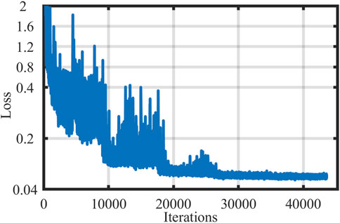
FIGURE 6. Training curves of the natural network.
where ci’ is the predicted value and ci is the true value.
Figure 7 illustrates the RMSE value of the test datasets; the lower the RMSE value, the closer the predicted sub-wavefront to the actual value. When the RMSE value is less than 0.1, we consider that the network has made an accurate prediction for the sub-wavefront. Furthermore, the accuracy of the network, r, is expressed as the ratio of the number of accurate predictions to the test datasets. The trained network has an accuracy of r = 98.73%, which means that it has the ability to predict sub-wavefront information with high accuracy and stability.
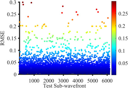
FIGURE 7. RMSE value of test datasets.
3.2 Wavefront reconstruction
As shown in Figure 5 in Section 3.1.1, the sub-wavefront information in full light is predicted using the trained network, and COG is utilized to obtain the slope information in a non-full-light subaperture. Finally, the modified algorithm completes the wavefront reconstruction. Neglecting the time-consuming constraint of reconstructing the wavefront when parallel computation of sub-wavefront information is used, the reconstruction time for a wavefront takes approximately 2 ms.
The wavefront reconstruction result for different sampling rates is shown in Figure 8, and the leftmost figure shows the match relationship between the optical pupil and MLA. This is followed in turn by the incident wavefront, reconstructed wavefront, and residual wavefront. d/r0 = 1, and the reconstructed Zernike modes for 6 × 6, 8 × 8, and 10 × 10 MLA are 46, 84, and 132, respectively. The corresponding PV, RMS, and relative error (RE) values are also shown in the figure. The definition of RE is given by Eq. 11, and RMSresidual and RMSwf represent the RMS values of the residual and incident wavefronts, respectively.
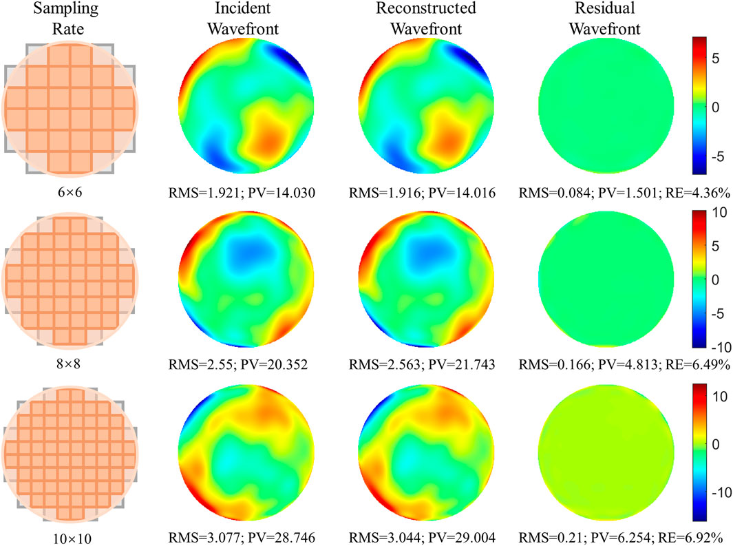
FIGURE 8. Reconstruction results of different sampling rates.
When the RE value is less than 10%, it means that the wavefront reconstruction algorithm can accurately reconstruct the wavefront. All the RE values in Figure 8 are less than 10%, providing sufficient evidence that the proposed method can accurately reconstruct the wavefront. Figure 8 shows large errors in the residual wavefront edge. This is because only the slope information has been obtained from the non-full-light subapertures, which are distributed at the edge of the incident wavefront, leading to a decrease in accuracy at the edge.
Furthermore, in order to be able to reflect the advantages of the proposed algorithm, it should be compared with the traditional method. The proposed algorithm and the traditional method with the same sampling rate (8 × 8) are used to reconstruct the wavefront, with atmospheric parameter d/r0 = 1 and 132 Zernike modes. The reconstructed and residual wavefronts are shown in Figure 9. For the proposed method’s reconstructed results, the RMS and PV values of the residual wavefront are 0.16 rad and 3.871 rad, respectively. Compared with the traditional method, the RMS and PV values of the residual wavefront are reduced by 88.4% and 85.85%, respectively.
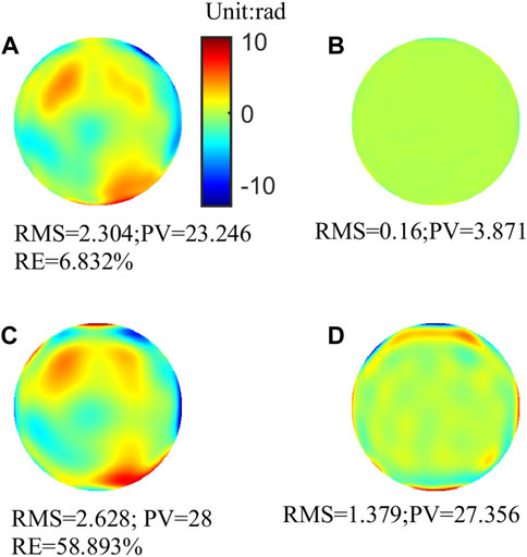
FIGURE 9. (A) Reconstructed wavefront of the proposed method; (B) residual wavefront of the proposed method; (C) reconstructed wavefront of the traditional method; and (D) residual wavefront of the traditional method.
To further investigate the generalization of the proposed method, in the same manner as in the previous paragraph, 1,000 wavefronts are randomly generated. The reconstructed statistical results using the two methods are shown in Figure 10. Almost all RE values of the proposed method are less than 10%. Obviously, compared with the traditional method, with the same sampling rate, the proposed method is able to reconstruct the wavefront with higher accuracy.
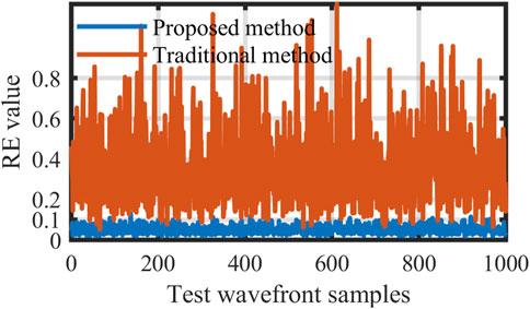
FIGURE 10. Results of reconstructing 1000 random wavefronts using proposed method (8×8) and traditional method (8×8).
Similarly, the 1,000 random wavefronts satisfy the atmospheric parameter D/r0 = 10 (where D is the diameter of the pupil); these are represented by 80-order Zernike modes. We reconstruct the wavefront using the traditional method (the sampling rate is 10 × 10) and the proposed algorithm (the sampling rate is 6 × 6), respectively. Figure 11 shows that almost all RE values are less than 0.1, the average RE value of the proposed method is 4.72%, and the average RE value of the traditional method is 2.12%. As observed from the result, using the proposed algorithm with a 6 × 6 sampling rate yields comparable results to the traditional method with a 10 × 10 sampling rate, although there will be a slight degradation in accuracy.
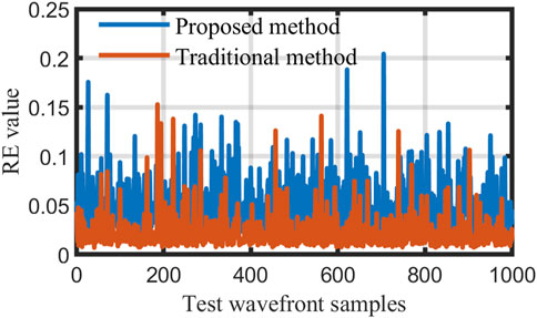
FIGURE 11. Results of reconstructing 1000 random wavefronts using proposed method (6×6) and traditional method (10×10).
4 Discussion
4.1 Sub-wavefront fitting error
It is worth exploring the ability of the new sub-wavefront assumption to fit sub-wavefronts. So, for plane fitting and quadratic surface fitting, 1,000 sub-wavefronts are generated for each case, which is similar to the generation of the datasets. Table 2 shows the statistical results, including the average, standard deviation, and average RE values. As can be seen from the results, under the same atmospheric conditions, using quadratic surface fitting can fit the sub-wavefront more accurately. However, as d/r0 increases, the fitting error also increases. Referring to the conventional Shack–Hartmann, in the case of d/r0 = 1, fitting a sub-wavefront with a plane has been widely used in engineering; the average and standard deviation of the RMS values of the residual wavefront are 0.154 rad and 0.121 rad, respectively, which indicates that the error of plane fitting is acceptable.
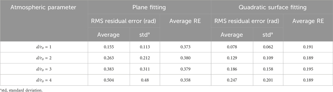
TABLE 2. Statistical comparison of different fitting methods.
Taking the plane fitting error as a reference value at d/r0 = 1, the residual wavefront RMS of quadratic surface fitting at d/r0 = 1 and d/r0 = 2 is well within the permissible error range. Therefore, the proposed method can be used to reconstruct the wavefront in these cases. Similarly, at d/r0 = 3, the average value is 0.186 rad and the standard deviation is 0.158 rad. The error exceeds the reference value, but it is still negligible and perhaps can be used to reconstruct the wavefront. In addition, for sub-wavefront with different atmospheric parameters, the RE values of the two fitting approaches are almost constant; therefore, as the d/r0 value increases, the fitting error also increases, and it is hard to reconstruct the wavefront.
4.2 Spatial resolution of reconstruction wavefronts
The proposed algorithm can accurately reconstruct wavefronts; however, it is still necessary to investigate how the spatial resolution can be improved. Therefore, for different d/r0 values and different sampling rates, 1,000 random aberrations are generated to analyze the resolution. As shown in Figure 12, in the case where d/r0 = 1 and the sampling rates are 6 × 6, 8 × 8, and 10 × 10 for the proposed method, the spatial resolutions are 84, 124, and 164 Zernike modes, respectively. For the traditional method, the spatial resolutions are 48, 60, and 80 Zernike modes, respectively. Obviously, at the same sampling rate, the proposed algorithm can reconstruct wavefronts with higher spatial resolution; at the same spatial resolution, the proposed algorithm can reconstruct wavefronts with lower sampling rates.
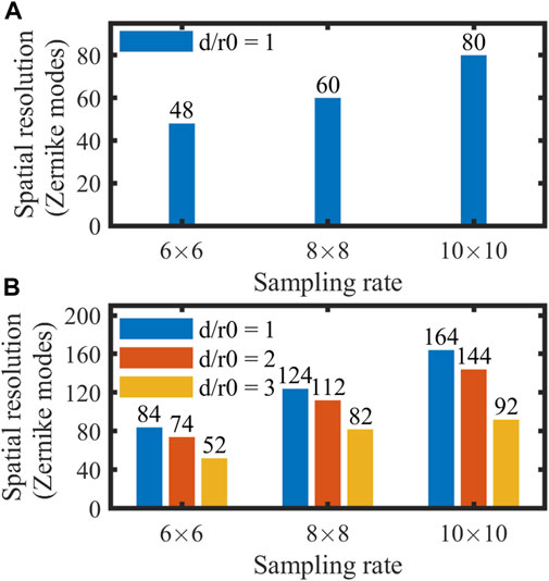
FIGURE 12. Spatial resolution of measurement with different MLA sampling rates for different atmospheric parameters. (A) Traditional method. (B) Proposed method.
In addition, in the cases where d/r0 = 2 and d/r0 = 3, the traditional method faces challenges in determining wavefront measurements. However, for the proposed algorithm, the spatial resolutions are 52, 82, and 92 Zernike modes, respectively. When d/r0 = 3, the wavefront can still be reconstructed accurately, even if the spatial resolution is degraded.
Therefore, the proposed algorithm can be applied to measure wavefront in a faint source or strong turbulence (d/r0<3) environment, or in the case of limited sampling rates, can be used to reconstruct wavefront with high spatial resolution.
4.3 Analyzing factors affecting spatial resolution
As can be seen from Figure 12, with the increase in the atmospheric parameter d/r0, the spatial resolution of the measurement degrades. There are two main reasons for this: on the one hand, as shown in Table 2, as d/r0 grows larger, the average value and standard deviation value of residual sub-wavefront RMS also increase, which implies that measurement accuracy will decrease with the same spatial sampling rates. On the other hand, as shown in Figure 13, as the turbulence intensity increases, although the average slope does not surpass the dynamic range of the subaperture, the spot has already exceeded the region of the subaperture, so the wrong wavefront information will be obtained. At the same time, the adjacent sub-wavefront information extraction will also be affected.
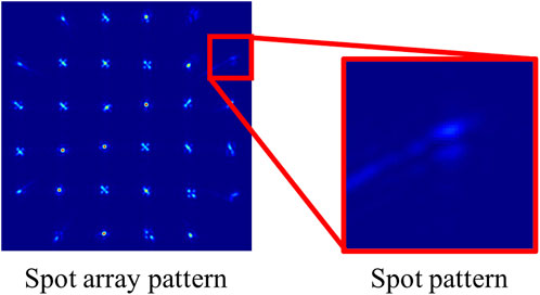
FIGURE 13. Spot array pattern and a spot pattern of high strength turbulence.
However, our proposed algorithm uses this imperfect information to reconstruct the wavefront at the cost of reduced spatial resolution. Using more parameters to more accurately express the sub-wavefront and effectively filtering out error information can help maintain its spatial resolution, which is on our agenda for future work.
5 Conclusion
In this paper, we establish a new assumption that treats the sub-wavefront as a quadratic surface and propose a method to extract the sub-wavefront information based on a neural network. So long as the spots have consistent features, even with different sampling rates, the trained network can also be used to predict the sub-wavefront information. This approach generates large datasets quickly, the network model is simple, and the reconstruction of a wavefront takes approximately 2 ms.
At the same time, the wavefront reconstruction algorithm is modified, introducing quadratic information into the reconstruction matrix so that the wavefront can be reconstructed with high speed, high precision, and high spatial resolution. In addition, the algorithm can be used in the case where d/r0 = 1–3, which breaks the limitation of d/r0 = 1. In conclusion, the proposed method allows us to sense the higher frequency aberrations and reconstruct the wavefront under faint-source or high-strength-turbulence conditions.
Data availability statement
The original contributions presented in the study are included in the article/Supplementary material; further inquiries can be directed to the corresponding authors.
Author contributions
HoG: conceptualization, formal analysis, investigation, methodology, software, validation, writing–original draft, writing–review and editing, and data curation. WZ: conceptualization, data curation, formal analysis, investigation, methodology, software, validation, writing–original draft, and writing–review and editing. SW: conceptualization, data curation, funding acquisition, investigation, methodology, resources, validation, and writing–original draft. KY: formal analysis, software, and writing–review and editing. MZ: formal analysis, software, and writing–review and editing. SL: software and writing–review and editing. HaG: writing–review and editing. PY: investigation, validation, and writing–review and editing.
Funding
The author(s) declare that financial support was received for the research, authorship, and/or publication of this article. This study was supported by the National Natural Science Foundation of China (11704382, 61805251, 61875203, and 62105336), Youth Innovation Promotion Association of the Chinese Academy of Science (Y2021103), and Foundation Incubation Fund of the Chinese Academy of Science (JCPYJJ-22005).
Conflict of interest
The authors declare that the research was conducted in the absence of any commercial or financial relationships that could be construed as a potential conflict of interest.
Publisher’s note
All claims expressed in this article are solely those of the authors and do not necessarily represent those of their affiliated organizations, or those of the publisher, the editors, and the reviewers. Any product that may be evaluated in this article, or claim that may be made by its manufacturer, is not guaranteed or endorsed by the publisher.
References
1. Platt BC, Shack R. History and principles of Shack-Hartmann wavefront sensing. J refractive Surg (2001) 17:S573–7. doi:10.3928/1081-597X-20010901-13
2. Yang J-T, Yang C-J, Wang K-H, Chang J-C, Wu C-Y, Chang C-Y. Remote focusing with dynamic aberration elimination by model-based adaptive optics. Opt Laser Tech (2024) 169:110126. doi:10.1016/j.optlastec.2023.110126
3. Christaras D, Tsoukalas S, Papadogiannis P, Börjeson C, Volny M, Lundström L, et al. Central and peripheral refraction measured by a novel double-pass instrument. Biomed Opt Express (2023) 14:2608–17. doi:10.1364/BOE.489881
4. Romashchenko D, Lundström L. Dual-angle open field wavefront sensor for simultaneous measurements of the central and peripheral human eye. Biomed Opt express (2020) 11:3125–38. doi:10.1364/BOE.391548
5. Galaktionov I, Sheldakova J, Nikitin A, Toporovsky V, Kudryashov A. A hybrid model for analysis of laser beam distortions using Monte Carlo and shack–hartmann techniques: numerical study and experimental results. Algorithms (2023) 16. doi:10.3390/a16070337
6. Miglani R, Malhotra JS. Performance enhancement of high-capacity coherent DWDM free-space optical communication link using digital signal processing. Photonic Netw Commun (2019) 38:326–42. doi:10.1007/s11107-019-00866-8
7. Bowman RW, Padgett MJ. An SLM-based Shack–Hartmann wavefront sensor for aberration correction in optical tweezers. J Opt (2010) 12:124004. doi:10.1088/2040-8978/12/12/124004
8. Wu X, Huang L, Gu N, Tian H, Wei W. Study of a Shack-Hartmann wavefront sensor with adjustable spatial sampling based on spherical reference wave. Opt Lasers Eng (2023) 160:107289. doi:10.1016/j.optlaseng.2022.107289
9. Rousset G, Lacombe F, Puget P, Gendron E, Arsenault R, Kern PY, et al. Status of the VLT Nasmyth adaptive optics system (NAOS). Proc SPIE (2000) 4007:72–81. doi:10.1117/12.390304
10. Meimon S, Fusco T, Michau V, Plantet C. Sensing more modes with fewer sub-apertures: the LIFTed Shack–Hartmann wavefront sensor. Opt Lett (2014) 39:2835–7. doi:10.1364/OL.39.002835
11. Meimon S, Fusco T, Mugnier LM. LIFT: a focal-plane wavefront sensor for real-time low-order sensing on faint sources. Opt Lett (2010) 35:3036–8. doi:10.1364/OL.35.003036
12. Li C, Li B, Zhang S. Phase retrieval using a modified Shack–Hartmann wavefront sensor with defocus. Appl Opt (2014) 53:618–24. doi:10.1364/AO.53.000618
13. Zhao M, Zhao W, Yang K, Wang S, Yang P, Zeng F, et al. Shack–Hartmann wavefront sensing based on four-quadrant binary phase modulation. Photonics (2022) 9:575. doi:10.3390/photonics9080575
14. Zhu Z, Mu Q, Li D, Yang C, Cao Z, Hu L, et al. More Zernike modes’ open-loop measurement in the sub-aperture of the Shack–Hartmann wavefront sensor. Opt Express (2016) 24:24611–23. doi:10.1364/OE.24.024611
15. Feng F, Li C, Zhang S. Moment-based wavefront reconstruction via a defocused Shack–Hartmann sensor. Opt Eng (2018) 57:074106–6. doi:10.1117/1.OE.57.7.074106
16. Wu X, Huang L, Gu N. Enhanced-resolution Shack-Hartmann wavefront sensing for extended objects. Opt Lett (2023) 48:5691–4. doi:10.1364/OL.504057
17. Xu Z, Wang S, Zhao M, Zhao W, Dong L, He X, et al. Wavefront reconstruction of a Shack–Hartmann sensor with insufficient lenslets based on an extreme learning machine. Appl Opt (2020) 59:4768–74. doi:10.1364/AO.388463
18. He Y, Liu Z, Ning Y, Li J, Xu X, Jiang Z. Deep learning wavefront sensing method for Shack-Hartmann sensors with sparse sub-apertures. Opt Express (2021) 29:17669–82. doi:10.1364/OE.427261
19. Guo Y, Wu Y, Li Y, Rao X, Rao C. Deep phase retrieval for astronomical Shack–Hartmann wavefront sensors. Monthly Notices R Astronomical Soc (2022) 510:4347–54. doi:10.1093/mnras/stab3690
20. Jaganathan K, Eldar YC, Hassibi B. Phase retrieval: an overview of recent developments. Opt Compressive Imaging (2016) 279–312. doi:10.1109/MSP.2016.2565061
22. Leon SJ, Björck Å, Gander W. Gram-Schmidt orthogonalization: 100 years and more. Numer Linear Algebra Appl (2013) 20:492–532. doi:10.1002/nla.1839
Keywords: Shack–Hartmann wavefront sensor, high-resolution wavefront sensing, sub-wavefront information extraction, phase modulation, neural network
Citation: Guan H, Zhao W, Wang S, Yang K, Zhao M, Liu S, Guo H and Yang P (2024) Higher-resolution wavefront sensing based on sub-wavefront information extraction. Front. Phys. 11:1336651. doi: 10.3389/fphy.2023.1336651
Received: 11 November 2023; Accepted: 18 December 2023;
Published: 08 January 2024.
Edited by:
Mingjian Cheng, Xidian University, ChinaReviewed by:
Lianghua Wen, Yibin University, ChinaXiao Sun, Curtin University, Australia
Huigao Duan, Hunan University, China
Copyright © 2024 Guan, Zhao, Wang, Yang, Zhao, Liu, Guo and Yang. This is an open-access article distributed under the terms of the Creative Commons Attribution License (CC BY). The use, distribution or reproduction in other forums is permitted, provided the original author(s) and the copyright owner(s) are credited and that the original publication in this journal is cited, in accordance with accepted academic practice. No use, distribution or reproduction is permitted which does not comply with these terms.
*Correspondence: Shuai Wang, d2FuZ3NodWFpQGlvZS5hYy5jbg==; Ping Yang, cGluZ3lhbmcyNTE2QDE2My5jb20=