Spectral characterization of optical aberrations in fluidic lenses

We report an extensive numerical study and supporting experimental results on the spectral characterization of optical aberrations in macroscopic fluidic lenses with tunable focal distance and aperture shape. By using a Shack–Hartmann wavefront sensor, we experimentally reconstruct the near-field wavefront transmitted by the fluidic lenses, and we characterize the chromatic aberrations in terms of Zernike polynomials in the visible range. Moreover, we further classify the spectral response of the lenses using clustering techniques, in addition to correlation and convolution measurements. Experimental results are in agreement with numerical results based on our theoretical model of the nonlinear deformation of thin elastic membranes.

1 Introduction

One of the most common ocular disorders worldwide, and the main cause of visual impairment in children, is myopia. Elongation of the axial length in the eyes, which characterizes medium and high levels of myopia, can increase the risk of severe ocular pathologies, potentially leading to irreversible blindness. Most traditional adaptive eye-wear based on fluidic lenses aim to correct refractive errors requiring medium dioptric power, such as mild myopia, hyperopia, and other focus errors [5, 6]. On the other hand, refractive errors other than focus, including coma, astigmatism, and higher-order aberrations, are usually treated via astigmatic corrections [1–3], which are more difficult to achieve with standard fluidic lenses. Moreover, in most cases, compounded errors are present, most commonly presbyopia with focus defects, requiring multi-focal lenses, the limited accommodation distance and highly restricted field-of-view of which can lead to high loss of visual capacity [4]. Finally, patients with severe visual impairment due to glaucoma or other visual traumas require large dioptric power corrections, necessitating thick organic lenses, which are prone to high-order aberrations, in addition to being significantly unattractive and unpractical. In a previous publication [7], we presented the first macroscopic fluidic lens eye-wear prototype with high dioptric power (+25 D to +100 D range) with optical aberrations below a fraction of the wavelength, which can adaptively restore accommodation distance within several centimeters, thus enabling access to the entire field-of-view. The lens is made of a PDMS-type elastic polymer which can adaptively modify its optical power according to the fluidic volume mechanically pumped in. Such a liquid lens exhibits a large dynamic range, and its focusing properties are polarization-independent [8]. Additionally, we demonstrated that by tuning the lens aperture, it is possible to address different optical aberrations, thus providing an additional degree of freedom for the lens design. Our design is attractive for adaptive eye-wear, in addition to cellular phones, cameras, optical zooms, or other machine vision applications where large magnification can be required [9; 12–23; 26].

In this paper, we present an extensive numerical and experimental spectral study of optical aberrations in macroscopic fluidic lenses with high dioptric power, tunable focal distance, and aperture shape [7], based on an empirical characterization of the refractive index of thin elastic membranes, such as PDMS, according to the Sellmeier model [10; 11]. Using a Shack–Hartmann wavefront sensor, we experimentally reconstruct the near-field wavefront transmitted by such fluidic lenses, and we characterize the chromatic aberrations in terms of Zernike polynomials over the visible wavelength range (λ = 400–650 nm) by using a programmable LED source. Moreover, we further classify the spectral response of the lenses using clustering techniques in addition to correlation and convolution measurements. Experimental results are in agreement with those of our theoretical model of nonlinear elastic membrane deformation.

2 Theoretical model

2.1 Inclusion of gravity effects

We briefly recall the model used in [7] to simulate the fluid lens surface shape without considering gravity effects. The equations used are those derived by Berger [24] to determine the nonlinear, large deformation of thin isotropic elastic plates.

${\nabla }^{4}w-{\alpha }^2{\nabla }^{2}w=\frac{q}{D},(\mathrm{1a})$

$\frac{\partial u}{\partial x}+\frac{\partial v}{\partial y}+\frac{1}{2}{\left(\frac{\partial w}{\partial x}\right)}^2+\frac{1}{2}{\left(\frac{\partial w}{\partial y}\right)}^2=\frac{{\alpha }^2{h}^2}{12}.(\mathrm{1b})$

In these equations, $w\left(x,y\right)$ is the local z-displacement of the membrane, with the non-deformed state assumed to correspond to the z = 0 plane; $u\left(x,y\right)$ and $v\left(x,y\right)$ are the local x and y displacements, respectively; D is the membrane bending rigidity; and h is its thickness. The magnitude $q\left(x,y\right)$ corresponds to the applied z-load, and α is a constant to be determined from the same equations by imposing appropriate boundary conditions.

For the case of uniform load (constant q) and elliptic aperture, analytical solutions of system 1) were obtained by the method of constant deflection contour lines derived by Mazumdar [25]. If the aperture in the plane z = 0 is an ellipse of x and y semi-axes a and b, respectively, the z-displacement of the membrane is given by

$w\left(\varsigma \right)=\frac{\mathrm{\Delta }V}{\pi ab}\frac{2\gamma \left[\gamma \left(1-{\varsigma }^2\right)I_1\left(2\gamma \right)+I_0\left(2\gamma \varsigma \right)-I_0\left(2\gamma \right)\right]}{\left({\gamma }^2+2\right)I_1\left(2\gamma \right)-2\gamma I_0\left(2\gamma \right)},(2)$

where ΔV is the volume of the liquid. The variable ς is defined as

${\varsigma }^2=x^2/a^2+y^2/b^2,(3)$

and the constant γ is related to ΔV by

$\mathrm{\Delta }V=\pi abh\frac{\sqrt{3a^4+2a^2{b}^2+3b^4}}{a^2+b^2}G\left(\gamma \right),(4)$

where

$G\left(\gamma \right)=\frac{\left({\gamma }^2+2\right)I_1\left(2\gamma \right)-2\gamma I_0\left(2\gamma \right)}{\sqrt{24\gamma }\sqrt{3\gamma {\left[I_1\left(2\gamma \right)\right]}^2-2I_2\left(2\gamma \right)\left[\gamma I_0\left(2\gamma \right)+2I_1\left(2\gamma \right)\right]}}.(5)$

We now consider the effect of gravity when the (x, y) plane of the lens aperture is vertical. In Eq. 1in the study by Berger load q has the expression

$q=q_0-\rho g\left(x\sin \theta +y\cos \theta \right),$

where q₀ is the load at the lens center (x = y = 0), ρ is the mass density of the filling fluid, g is the acceleration of gravity, and θ is the angle between the vertical direction and the y-axis (see Figure 1).

FIGURE 1

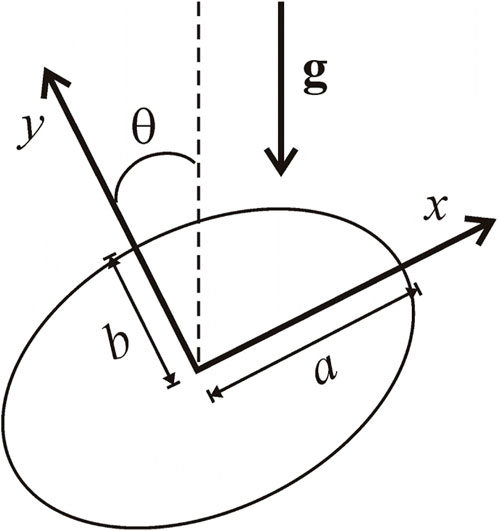
FIGURE 1. Notation used in the model to include the effect of gravity on the lens surface shape.

In the case that ρgL/q₀ ≪ 1, with L as the characteristic length of the lens pupil, we can treat gravity effects as a perturbation to the case with uniform load q₀, as previously obtained, and write

$\begin{array}{ccc}\hfill w& =\hfill & w_0+w_1,\hfill \\ \hfill \alpha & =\hfill & {\alpha }_0+{\alpha }_1,\hfill \end{array}$

with w₀ and α₀ corresponding to the solution of the case with q = q₀. Linearization of Eq.1a in the perturbations w₁ and α₁ yields

${\nabla }^4{w}_1-{\alpha }_0^2{\nabla }^2{w}_1-2{\alpha }_0{\alpha }_1{\nabla }^2{w}_0=-\frac{\rho g}{D}\left(x\sin \theta +y\cos \theta \right).(6)$

For a clamped membrane with no pre-stretching, u = v = 0 at ψ = 0, and so the integral of the linearized version of Eq.1b over the area S₀ of the lens aperture gives

$\underset{S_0}{\int }\left(\frac{\partial w_0}{\partial x}\frac{\partial w_1}{\partial x}+\frac{\partial w_0}{\partial y}\frac{\partial w_1}{\partial y}\right)dxdy=\frac{{\alpha }_0{\alpha }_1{h}^2}{6}{S}_0.(7)$

We now consider the solution to Eq. 6 in the usual case in which the membrane forces dominate: ${\alpha }_0^2{L}^2\gg 1$. In this case, except extremely close to the membrane border, one has $\left|{\nabla }^4{w}_1\right|\ll \left|{\alpha }_0^2{\nabla }^2{w}_1\right|$, and so it is easy to check that the solution to Eq. 6 satisfying the boundary condition w₁ = 0 at the border of the membrane is given by

$w_1=-\frac{2{\alpha }_1}{{\alpha }_0}{w}_0-\frac{\rho g{a}^2{b}^2}{2D{\alpha }_0^2}\left(1-\frac{x^2}{a^2}-\frac{y^2}{b^2}\right)\left(\frac{x\sin \theta }{a^2+3b^2}+\frac{y\cos \theta }{3a^2+b^2}\right).(8)$

Using expression 8) in Eq. 7, one readily obtains α₁ = 0 so that the complete solution with the inclusion of gravity effects is

$w=w_0-\frac{\rho g}{2D{\gamma }^2}\frac{a^4{b}^4\left(a^2+b^2\right)}{3a^2+2a^2{b}^2+3b^4}\left(1-\frac{x^2}{a^2}-\frac{y^2}{b^2}\right)\left(\frac{x\sin \theta }{a^2+3b^2}+\frac{y\cos \theta }{3a^2+b^2}\right),(9)$

where w₀ is the solution previously obtained for uniform load, Eq. 2, and the constant γ is the one determined in that solution using Eq. 4.

2.2 Determination of the aberrations of the fluid lens

In order to determine the aberrations of a fluid lens with one plane surface, we consider a plane wavefront with normal incidence on the plane side of the membrane, taken at z = 0 (see Figure 2). The corresponding rays, parallel to the z-axis of unit vector e_z, are then refracted according to Snell’s law when they cross the membrane curved surface at $z=w\left(x,y\right)$. The external normal unit vector at that surface is given by (in Cartesian components)

$\mathbf{n}=\frac{\left(-w_x,-w_{y,}1\right)}{\sqrt{1+w_x^2+w_y^2}},(10)$

where the subscripts x and y indicate derivatives with respect to the corresponding coordinate.

FIGURE 2

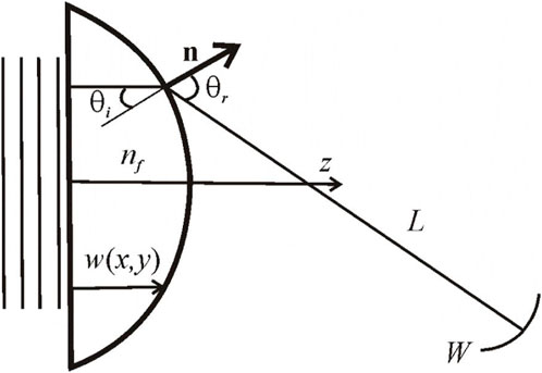
FIGURE 2. Notation used in the model for the ray tracing from a plane wavefront incident on the plane surface of the lens to the refracted wavefront W.

The angle θ_i of the rays incident from inside the lens, relative to the external normal direction at the corresponding point of the membrane curved surface, is thus given by

$\cos {\theta }_i=\mathbf{n}\cdot {\mathbf{e}}_z=\frac{1}{\sqrt{1+w_x^2+w_y^2}}.(11)$

The Snell law then determines the angle of the refracted ray emerging from the lens, also relative to the normal direction, as

$\sin {\theta }_r=n_f\frac{\sqrt{w_x^2+w_y^2}}{\sqrt{1+w_x^2+w_y^2}},(12)$

where n_f is the index of refraction of the filling fluid, relative to that of air.

The refracted ray is contained in the plane determined by the normal unit vector n and the unit vector tangent to the surface

$\mathbf{t}=\frac{{\mathbf{e}}_z-\left(\mathbf{n}\cdot {\mathbf{e}}_z\right)\mathbf{n}}{\left|{\mathbf{e}}_z-\left(\mathbf{n}\cdot {\mathbf{e}}_z\right)\mathbf{n}\right|}=\frac{\left(w_x,w_{y,}{w}_x^2+w_y^2\right)}{\sqrt{\left(1+w_x^2+w_y^2\right)\left(w_x^2+w_y^2\right)}},(13)$

so that the ray direction is given by the unit vector

${\mathbf{k}}_r=\mathbf{n}\cos {\theta }_r+\mathbf{t}\sin {\theta }_r.(14)$

The explicit expressions of the Cartesian components of k_r are

$k_{rx,y}=\frac{n_f-\sqrt{1+\left(1-n_f^2\right)\left(w_x^2+w_y^2\right)}}{1+w_x^2+w_y^2}{w}_{x,y},(\mathrm{15a})$

$k_{rz}=\frac{n_f\left(w_x^2+w_y^2\right)+\sqrt{1+\left(1-n_f^2\right)\left(w_x^2+w_y^2\right)}}{1+w_x^2+w_y^2},(\mathrm{15b})$

which are functions of the point (x, y) in the plane z = 0, at which the ray originated.

In this way, a generic ray starting at the point (x, y) in the plane z = 0 inside the lens is refracted at the point ${\mathbf{X}}_0=\left(x,y,w\left(x,y\right)\right)$ on the membrane surface, and after traversing in air a distance L reaches the point X_L = X₀ + k_rL so that (from now on, we do not write the explicit dependence on (x, y) of w and of k_r)

$z_L=w+k_{rz}L,(16)$

and

$x_L=x+\frac{k_{rx}}{k_{rz}}\left(z_L-w\right),(\mathrm{17a})$

$y_L=y+\frac{k_{ry}}{k_{rz}}\left(z_L-w\right).(\mathrm{17b})$

The phase at (x_L, y_L, z_L) is thus

${\varphi }_L={\varphi }_0+\frac{2\pi }{\lambda }\left(n_{f}w+\frac{z_L-w}{k_{rz}}\right),(18)$

where ϕ₀ is the phase of the front at z = 0 and λ is the wavelength in air.

From (18), we can determine the z_W position of a wavefront of given phase ϕ_W as

$z_W=w\left(1-n_f{k}_{rz}\right)+k_{rz}\frac{\lambda }{2\pi }\left({\varphi }_W-{\varphi }_0\right),(19)$

to which correspond the (x_W, y_W) coordinates:

$x_W=x+k_{rx}\left[\frac{\lambda }{2\pi }\left({\varphi }_W-{\varphi }_0\right)-n_{f}w\right],(\mathrm{20a})$

$y_W=y+k_{ry}\left[\frac{\lambda }{2\pi }\left({\varphi }_W-{\varphi }_0\right)-n_{f}w\right].(\mathrm{20b})$

These two relations can, in principle, be solved to give

$x=x\left(x_W,y_W\right),(\mathrm{21a})$

$y=y\left(x_W,y_W\right),(\mathrm{21b})$

which, if replaced in (19), give the wavefront geometry $z_W=z_W\left(x_W,y_W\right)$.

If this wavefront is analyzed at a position z_A, we can, without loss of generality, take this position as that of the image of the origin, x = y = 0: $z_A=w_0\left(1-n_f{k}_{rz0}\right)+k_{rz0}\frac{\lambda }{2\pi }\left({\varphi }_W-{\varphi }_0\right)$, where $w_0=w\left(\mathrm{0,0}\right)$ and $k_{rz0}=k_{rz}\left(\mathrm{0,0}\right)$ so that

$\frac{\lambda }{2\pi }\left({\varphi }_W-{\varphi }_0\right)=\frac{z_A-w_0\left(1-n_f{k}_{rz0}\right)}{k_{rz0}},(22)$

and analyze the deviation from a plane front: Δz_W = z_W − z_A, which is conveniently written as

$\mathrm{\Delta }{z}_W=w\left(1-n_f{k}_{rz}\right)-\frac{k_{rz}}{k_{rz0}}{w}_0\left(1-n_f{k}_{rz0}\right)+\left(\frac{k_{rz}}{k_{rz0}}-1\right)z_A.(23)$

The corresponding (x_W, y_W) coordinates are written as

$x_W=x+\frac{k_{rx}}{k_{rz0}}\left[z_A-w_0-n_f{k}_{rz0}\left(w-w_0\right)\right],(\mathrm{24a})$

$y_W=y+\frac{k_{ry}}{k_{rz0}}\left[z_A-w_0-n_f{k}_{rz0}\left(w-w_0\right)\right].(\mathrm{24b})$

In this way, Eqs 23, 24a, 24b give the wavefront geometry, analyzed at z = z_A, parameterized in terms of the (x, y) coordinates on the plane at z = 0.

We further model the wavefront analyzer at z = z_A as having a circular aperture of radius r_A so that the section of the wavefront $\mathrm{\Delta }{z}_W\left(x_W,y_W\right)$ to be studied is expressed as $\mathrm{\Delta }{z}_W\left(r_A\xi \cos \varphi ,r_A\xi \sin \varphi \right)$, with 0 ≤ ξ ≤ 1, and decomposed in Zernike polynomials in polar coordinates $Z_n\left(\xi ,\varphi \right)$,

$\mathrm{\Delta }{z}_W=\sum _n{a}_n{Z}_n\left(\xi ,\varphi \right),(25)$

with

$a_n=\frac{1}{\pi }{\int }_0^{2\pi }{\int }_0^1\mathrm{\Delta }{z}_W\left(r_A\xi \cos \varphi ,r_A\xi \sin \varphi \right)Z_n\left(\xi ,\varphi \right)\xi d\xi d\varphi .(26)$

We have followed the standard OSA/ANSI indexing and normalization scheme, used in the Shack–Hartmann wavefront sensor, for which the first 15-term orthonormal Zernike circle polynomials are as follows:

$\begin{array}{ccc}\hfill Z_0& =\hfill & 1,\hfill \\ \hfill Z_1& =\hfill & 2\xi \sin \varphi ,\hfill \\ \hfill Z_2& =\hfill & 2\xi \cos \varphi ,\hfill \\ \hfill Z_3& =\hfill & \sqrt{6}{\xi }^2\sin 2\varphi ,\hfill \\ \hfill Z_4& =\hfill & \sqrt{3}\left(2{\xi }^2-1\right),\hfill \\ \hfill Z_5& =\hfill & \sqrt{6}{\xi }^2\cos 2\varphi ,\hfill \\ \hfill Z_6& =\hfill & \sqrt{8}{\xi }^3\sin 3\varphi ,\hfill \\ \hfill Z_7& =\hfill & \sqrt{8}\left(3{\xi }^3-2\xi \right)\sin \varphi ,\hfill \\ \hfill Z_8& =\hfill & \sqrt{8}\left(3{\xi }^3-2\xi \right)\cos \varphi ,\hfill \\ \hfill Z_9& =\hfill & \sqrt{8}{\xi }^3\cos 3\varphi ,\hfill \\ \hfill Z_{10}& =\hfill & \sqrt{10}{\xi }^4\sin 4\varphi ,\hfill \\ \hfill Z_{11}& =\hfill & \sqrt{10}\left(4{\xi }^4-3{\xi }^2\right)\sin 2\varphi ,\hfill \\ \hfill Z_{12}& =\hfill & \sqrt{5}\left(6{\xi }^4-6{\xi }^2+1\right),\hfill \\ \hfill Z_{13}& =\hfill & \sqrt{10}\left(4{\xi }^4-3{\xi }^2\right)\cos 2\varphi ,\hfill \\ \hfill Z_{14}& =\hfill & \sqrt{10}{\xi }^4\cos 4\varphi .\hfill \end{array}$

3 Spectral response

In order to characterize the spectral response of the polydimethylsiloxane (PDMS-type) elastic membrane used to fabricate the fluidic lenses, we incorporate an empirical expression for the refractive index of PDMS Sylgard 184, as reported in [10]. The refractive index n(λ) decreases for increasing wavelength λ, which is typical of glass and polymeric materials. For the approximation of the dispersion across the entire visible light spectrum, the Sellmeier dispersion model is used, which describes the empirical relation between the refractive index n(λ) and the wavelength λ, given by

$n{\left(\lambda \right)}^2=1+\frac{B_1{\lambda }^2}{{\lambda }^2-C_1}+\frac{B_2{\lambda }^2}{{\lambda }^2-C_2}+\frac{B_3{\lambda }^2}{{\lambda }^2-C_3},(27)$

where B₁, B₂, B₃, C₁, C₂, C₃ are the experimentally determined Sellmeier coefficients. As reported in Ref. [10], B₁ = 1.0093 and C₁ [nm²] = 13.185. Due to the limited number of measurement points (three wavelengths with eight measurements each), the second and third Sellmeier coefficients are set to 0 [10]. A plot of the refractive index vs wavelength within the range 400 nm–1,500 nm is presented in Figure 3.

FIGURE 3

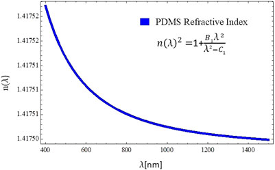
FIGURE 3. PDMS refractive index (n(λ)) vs wavelength (λ). The refractive index is obtained by experimentally determining the Sellmeier coefficients (B₁, C₁), resulting in $n{(\lambda )}^2=1+\frac{B_1{\lambda }^2}{{\lambda }^2-C_1}$, with B₁= 1.0093 and C₁ [nm²] = 13.185 [10].

According to the theoretical model, the spectral response of the phase P (x, y, λ) acquired by the beam upon propagation over a distance z_d can be expressed as

$P\left(x,y,\lambda \right)=\frac{2\pi }{\lambda }\left[n\left(\lambda \right)\ast w+\left(z_d-w\right)\ast k_z\left(\lambda \right)\right],(28)$

where w is the local displacement in the z-direction and k_z is given by

$k_z\left(\lambda \right)=\frac{1+\left(w_x^2+w_y^2\right)}{n\left(\lambda \right)\left(w_x^2+w_y^2\right)+\sqrt{1+\left(1-n{\left(\lambda \right)}^2\right)\left(w_x^2+w_y^2\right)}}.(29)$

We performed numerical simulations of the phase acquired by the beam upon propagation over a distance z_d = 3.5 cm. Numerical simulations are displayed in Figure 4. Density plots of P (x, y) for λ = 600 nm are displayed in Figures 4A, C. Figures 4B, D display the corresponding contour plots. Simulations are reported for fluidic lenses with circular apertures (top row: circular aperture with horizontal and vertical axes a = b = 1.7 cm) and for fluidic lenses with elliptic apertures (bottom row: elliptic aperture with horizontal and vertical axes a = 1.3 cm and b = 1.7 cm).

FIGURE 4

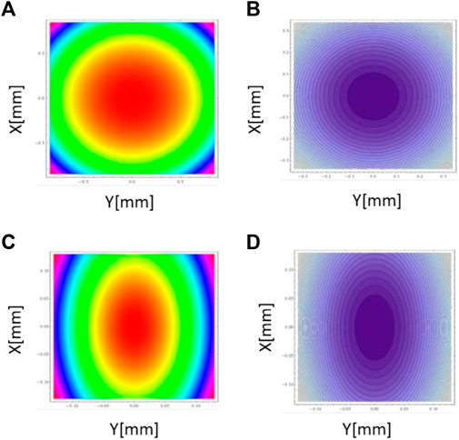
FIGURE 4. (A) and (C) Density plots of acquired phase P (x, y) upon propagation over a distance z_d = 3.5 cm, for λ = 600 nm. (B) and (D) Corresponding contour plots. Top row: circular aperture with horizontal and vertical axes a = b = 1.7 cm. Bottom row: elliptic aperture with horizontal and vertical axes a = 1.3 cm and b = 1.7 cm, respectively.

3.1 Wavefront aberrations of a single membrane

In order to characterize numerically the spectral response of optical aberrations and compare directly with experimental data, we expanded the wavefront aberrations of a single elastic membrane in terms of Zernike polynomials up to order 14, for a beam with wavelength λ) in the range 400–1,500 nm, thus numerically characterizing the spectral response in the visible and infrared domains. Even though we analyze wavefront aberrations in terms of Zernike polynomials up to order 14, we only display those coefficients for Zernike polynomials which are not negligible, namely, P₀, P₂, P₃, P₆ (for circular apertures) and P₀, P₂, P₃, P₅ (for elliptic apertures). The remaining Zernike coefficients are all below 10^–14, so they are not displayed in the figures.

Numerical results of wavefront aberrations for fluidic lenses with circular aperture (axes a = b = 1.7 cm) are displayed in Figure 5. Figures 5A–D, correspond to normalized Zernike coefficients for polynomials of orders P₀, P₂, P₃, and P₆, respectively. The remaining polynomials are not reported because their coefficients are negligible (≪ 10^–14). Numerical results for the chromatic response of fluidic lenses with elliptic apertures characterized by ellipse axes (a = 1.5 cm, b = 1.7 cm) and (a = 1.3 cm, b = 1.7 cm) are displayed in Figures 6, 7, respectively. Figures 6A–D and Figures 7A–D correspond to Zernike coefficients for polynomials of orders P₀, P₂, P₃, and P₅, respectively. The remaining polynomials are not displayed because their coefficients are negligible. As it is apparent from numerical results, the dependence of wavefront aberrations is of the general form |1/λ|. Moreover, spectral fluctuations in wavefront aberrations are within a fraction of λ.

FIGURE 5

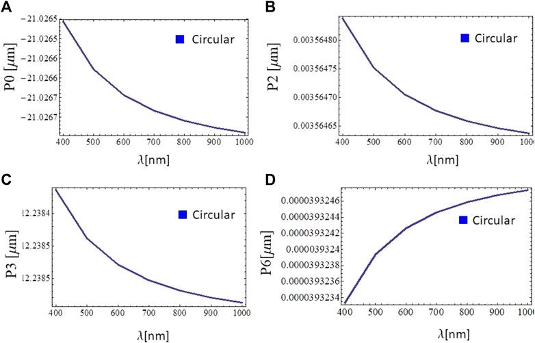
FIGURE 5. Numerical simulations of optical aberrations based on the expansion of the wavefront in terms of Zernike polynomials over the visible range λ = 400 − 1,500 nm, for fluidic lenses with a circular aperture characterized by axes (a = 1.7 cm, b = 1.7 cm) (A), (B), (C), and (D), correspond to Zernike coefficients in [μm] for polynomials of orders P₀, P₂, P₃, P₆, respectively. Zernike coefficients characterizing the remaining polynomials are negligible (≪ 10^–14). Further details are in the text.

FIGURE 6

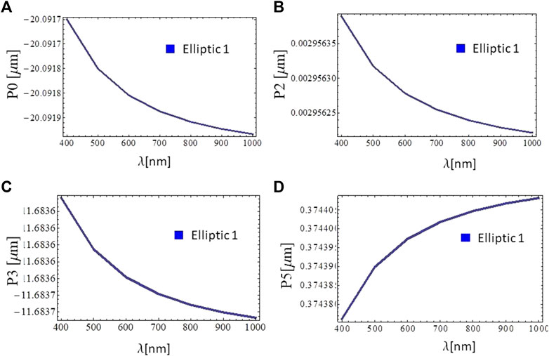
FIGURE 6. Numerical simulations of optical aberrations based on the expansion of the wavefront in terms of Zernike polynomials over the visible range λ = 400–1,500 nm, for fluidic lenses with an elliptic aperture characterized by axes (a = 1.5 cm, b = 1.7 cm) (A), (B), (C), and (D) correspond to Zernike coefficients in [μm] for polynomials of orders P₀, P₂, P₃, and P₅, respectively. Zernike coefficients characterizing the remaining polynomials are negligible (≪10^–14). Further details are in the text.

FIGURE 7

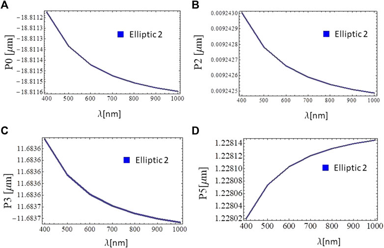
FIGURE 7. Numerical simulations of optical aberrations based on the expansion of the wavefront in terms of Zernike polynomials over the visible range λ =400–1,500 nm, for fluidic lenses with an elliptic aperture characterized by axes (a =1.3 cm, b =1.7 cm) (A), (B), (C), and (D) correspond to Zernike coefficients in [μm] for polynomials of orders P₀, P₂, P₃, and P₅, respectively. Zernike coefficients characterizing the remaining polynomials are negligible (≪ 10^–14). Further details are in the text.

3.2 Fluidic lens prototype

As readily reported in a previous publication [7], the fluidic lens consists of two layers of the elastic membrane of the polydimethylsiloxane (PDMS-type). The two elastic films are held together by an aluminum frame, sealed with the elastic membrane. An optical fluid of refractive index matched to the polymer, such as glycerol or distilled water, is injected between the elastic layers. By increasing or decreasing the fluid volume mechanically injected, it is possible to tune the focal distance across several centimeters and adjust the optical power of the lens. Furthermore, we tune one additional degree of freedom, given by the shape of the aperture. By modifying the aperture shape from circular (Figure 8B ) to elliptical (Figure 8C ), we can introduce different optical corrections. The typical size for the circular lens is given by a diameter d = 17 mm, and the elliptic lenses have a major axis b = 17 mm and minor axes a = 15 mm and a = 13 mm. Please note the axes labeling used in the theoretical model is not necessarily the same as the axes labelling used in the experimental setup. Further details regarding the fabrication of the fluidic lens prototype are reported in a previous article [7].

FIGURE 8

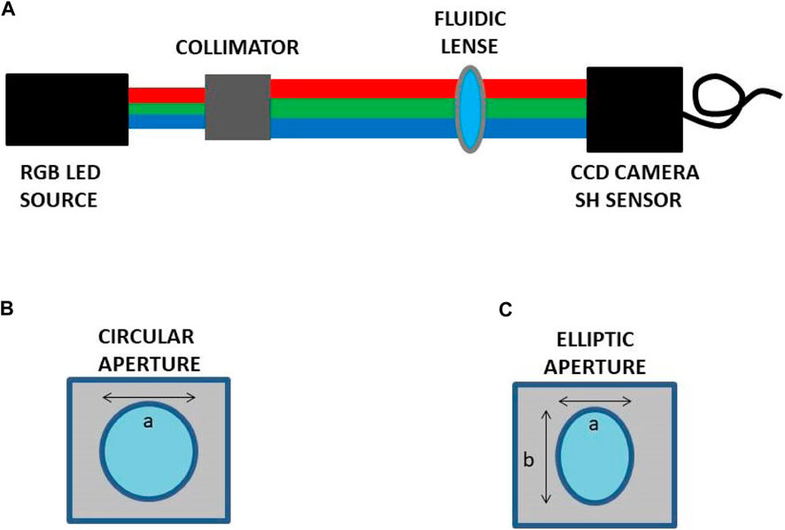
FIGURE 8. (A) Experimental scheme for reconstruction of the wavefront transmitted by the fluidic lens prototype and characterization of the chromatic response of optical aberrations using a collimated incoherent programmable LED source (ALIC Smart Life) and a Shack–Hartmann wavefront sensor (Thorlabs WFS150-5C). Scheme of the fluidic lens prototype: (B) circular aperture (horizontal and vertical axes a = b = 17 mm) and (C) elliptic aperture (horizontal axes (1,2) a₁₍₂₎= 15 (13) mm and vertical axis b = 17 mm). By tuning the aperture of the lens, it is possible to address different optical aberrations.

4 Experimental results

4.1 Wavefront reconstruction

In order to characterize the chromatic response of the light field transmitted by the fluidic lenses, we reconstructed the wavefront transmitted through the lenses using a Shack–Hartmann wavefront sensor Figure 8A (Model Thorlabs WFS150-5C, raw experimental data can be found at our GitHub repository [27]). To this end, we used a collimated incoherent RGB LED source (RGB: red–green–blue). Perfect collimation of a polychromatic beam can never be achieved. Here, by collimation, we refer to the fact that we verified the beam size did not diverge significantly over large distances (3 m or more), and we also confirmed that the wavefront impinging on the fluidic lenses was nearly a plane wavefront so that we could use the internal calibration of the Shack–Hartmann wavefront sensor, and all measured wavefront aberrations could be ascribed to the fluidic lenses themselves.

Shack–Hartmann wavefront sensors (SHWSs) enable analyzing the shape of an incident beam’s wavefront by dividing the beam into an array of discrete intensity points using a micro-lens array. These data are then used to reconstruct and analyze the shape of the wavefront using Zernike polynomials. In addition to analyzing classical optics phenomena, they are increasingly employed in applications where real-time monitoring of the wavefront is required to control adaptive optics with the intent of removing the wavefront distortion before creating an image. In particular, SHWSs enable two types of wavefront characterizations. I) Direct measurement (not displayed in Figure 9): shows the wavefront that is directly calculated from the measured spot deviations using a 2-dimensional integration procedure. II) Zernike reconstruction (left column in Figure 9): displays the wavefront that is reconstructed using a selected set of the determined Zernike coefficients. The advantages of Zernike reconstruction are as follows: i) selecting only a few lower-order Zernike modes for reconstruction smooths the wavefront surface (noise canceling), ii) the lowest-order Zernike modes (for instance, Z0 piston, Z1 tip, and Z2 tilt) are always present, but they are of less interest. Using an appropriate reconstruction (e.g., starting from Z3) can omit the Z0, Z1, and Z3 Zernike modes in order to see only the higher-order modes. iii) If selecting particular Zernike modes, they can be displayed and analyzed separately. Difference (right column in Figure 9): displays the difference between the I) directly measured wavefront and II) reconstructed wavefront and is therefore an indicator of the fit error.

FIGURE 9

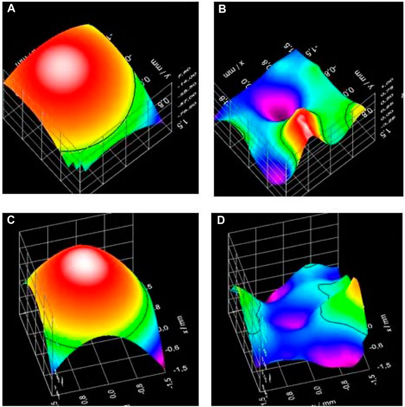
FIGURE 9. Experimentally reconstructed wavefront using a Shack–Hartmann sensor (Model Thorlabs WFS150-5C) and a collimated incoherent LED source. (A) Reconstructed wavefront produced by a fluidic lens with a circular aperture. (C) Reconstructed wavefront produced by a fluidic lens with an elliptic aperture. The qualitative difference in the wavefront due to the shape of the aperture is apparent. (B and D) Residual difference between measured and reconstructed wavefronts. Further details on the Shack–Hartmann wavefront sensor are provided in [7].

The incident field had a residual field curvature below λ/6. The sensor was placed 10 cm apart from the fluidic lens, with an aperture limited by the pupil size of the sensor itself, typically 3 mm in diameter. We reconstructed the wavefront produced by a circular fluidic lens filled with V_max = 6 mL corresponding to an optical power (OP) = 50 D (Figure 9A) and by an elliptical fluidic lens filled with V_min = 4 mL corresponding to OP = 36 D (Figure 9C). The qualitative difference in the wavefront due to the shape of the aperture is apparent. Residual differences between the measured wavefront and the reconstructed wavefront are displayed in Figures 9B, D). Further details on the Shack–Hartmann wavefront sensor are provided in Ref. [7].

4.2 Measured Zernike coefficients

In order to experimentally characterize the spectral response of optical aberrations in the central region of the fluidic lens prototype, we use the experimental setup described in Figure 8A. A collimated incoherent beam, produced by a programmable LED source (ALIC Smart Life, 14W, Luminous Flux 1400 lm, λ = 400–1,045 nm) propagates through the fluidic lens and is imaged by a Shack–Hartmann wavefront sensor (Model Thorlabs WFS150-5C), located at a distance of 2 cm from the fluidic lens, in order to image the near-field wave produced by the lens. The area of the beam to be characterized is determined by the aperture of the sensor (typically 3 mm). We verified that the transverse profile of the beam did not change significantly when tuning the wavelength of the source across the entire spectral range. Spectral characterizations in the visible range are mostly qualitative due to the broad spectrum produced by the incoherent LED source.

Measured aberrations in μm, in terms of the coefficients associated with Zernike polynomials of order 0 to 14, for red, green, and blue LED illumination are displayed in Figures 10A-I. First column: blue LED source, (A) circular aperture (a = b = 1.7 cm), (D) elliptic aperture 1 (a = 1.5 cm, b = 1.7 cm), and (G) elliptic aperture 2 (a = 1.3 cm, b = 1.7 cm). Second column: green LED source, (B) circular aperture (a = b = 1.7 cm), (E) elliptic aperture 1 (a = 1.5 cm, b = 1.7 cm), and (H) elliptic aperture 2 (a = 1.3 cm, b = 1.7 cm). Third column: red LED source, (C) circular aperture (a = b = 1.7 cm), (F) elliptic aperture 1 (a = 1.5 cm, b = 1.7 cm), and (I) elliptic aperture 2 (a = 1.3 cm, b = 1.7 cm).

FIGURE 10

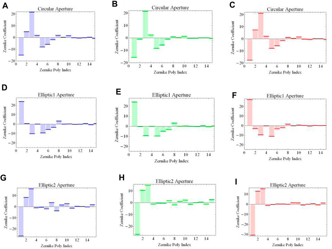
FIGURE 10. (A–I) Measured aberrations in μm, in terms of coefficients of associated Zernike polynomials of order 0 to 14, for blue, green, and red LED light. First column: blue LED source, (A) circular aperture (a = b = 1.7 cm), (D) elliptic aperture 1 (a = 1.5 cm, b = 1.7 cm) and (G) elliptic aperture 2 (a = 1.3 cm, b = 1.7 cm). Second column: green LED source, (B) circular aperture (a = b = 1.7 cm), (E) elliptic aperture 1 (a = 1.5 cm, b = 1.7 cm), and (H) elliptic aperture 2 (a = 1.3 cm, b = 1.7 cm). Third column: red LED source, (C) circular aperture (a = b = 1.7 cm), (F) elliptic aperture 1 (a = 1.5 cm, b = 1.7 cm), and (I) elliptic aperture 2 (a = 1.3 cm, b = 1.7 cm). The agreement with numerical simulations is mostly qualitative due to the spectral broadness of the LED source. Further details are in the text.

In order to quantify the agreement between experimental results and numerical simulations, we calculated the distance between measured Zernike coefficients for red–green–blue (RGB) wavelengths. We considered three different distance measures defined for two sets of data {a, b, c} and {x, y, z} in the following form: 1) Euclidean distance $D_1=\sqrt{|a-x{|}^2+|b-y{|}^2+|c-z{|}^2}$, 2) Canberra distance D₂ = |a − x|/(|a| + |x|) + |b − y|/(|b| + |y|) + |c − z|/(|c| + |z|), and 3) Bray–Curtis distance $D_3=(|a-x|+|b-y|+|c-z|)/\left((|a+x|+|b+y|+|c+z|)\right.$.

A brief comparison between the different distance measures is in order: D₁ corresponds to the “Pythagorean distance and is the only measure that can be subject to a direct geometrical interpretation; therefore, in this sense, it is the most intuitive one. D₂ and D₃ distance measures are similar in essence as they are both based on the algebraic concept of norm of a vector. They differ in the normalization factor. While D₂ normalizes each element of the vector independently, D₃ introduces a global normalization factor, and is therefore less sensitive (larger in modulus), as can be verified in Figures 11G, J. Note that D₁ is not normalized, and for this reason, it is typically larger in modulus than D₂ and D₃. We did not include the Manhattan distance in this analysis because it returned practically identical results to the Euclidean distance. The usefulness of the Manhattan measure was clearly revealed when employed in clustering techniques (see Section 2.4; Figure 12).

FIGURE 11

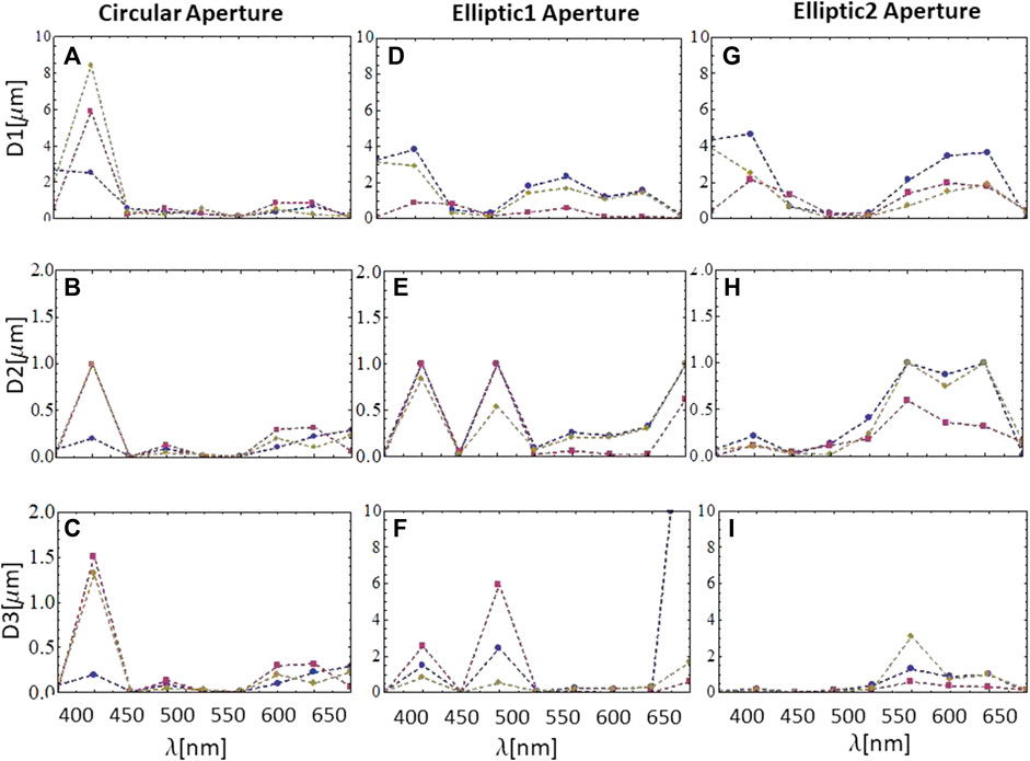
FIGURE 11. Comparison between spectral distances between measured Zernike coefficients in μm, as quantified by three different distance measures, D₁, D₂, and D₃, for red–green–blue (RGB) wavelengths. Blue markers, magenta markers, and brown markers correspond to B–R distance, B–G distance, and R–G distance, respectively. (A, B, and C) depict spectral distances D₁, D₂, and D₃ for fluidic lenses with circular apertures, respectively. (D, E, and F) depict spectral distances D₁, D₂, and D₃ for fluidic lenses with elliptic 1 aperture, respectively. (G, H, and I) depict spectral distances D₁, D₂, and D₃ for fluidic lenses with elliptic 2 aperture, respectively. Further details are in the text.

FIGURE 12

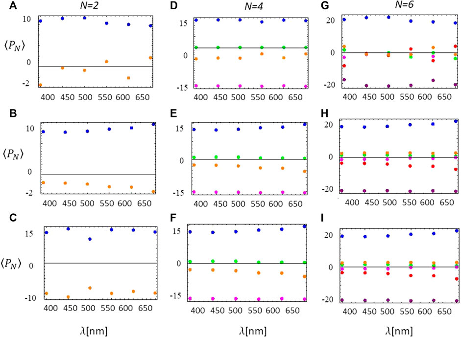
FIGURE 12. (A–I) Experimental clusters for average Zernike coefficients (⟨P_N⟩) in the range λ = 400–650 nm, partitioned into a predetermined set of N clusters with N = 2, 4, 6. First column: N = 2 clusters, (A) circular aperture (a = b = 1.7 cm), (B) elliptic aperture 1 (a =1.5 cm, b = 1.7 cm), and (C) elliptic aperture 2 (a = 1.3 cm, b = 1.7 cm). Second column N = 4 clusters, (D) circular aperture (a = b = 1.7 cm), (E) elliptic aperture 1 (a = 1.5 cm, b = 1.7 cm), and (F) elliptic aperture 2 (a = 1.3 cm, b = 1.7 cm). Third column: N = 6 clusters, (G) circular aperture (a = b = 1.7 cm), (H) elliptic aperture 1 (a = 1.5 cm, b = 1.7 cm), and (I) elliptic aperture 2 (a = 1.3 cm, b = 1.7 cm). Further details are in the text.

Comparison between spectral distances for measured Zernike coefficients in μm, for RGB wavelengths are displayed in Figure 10. Blue markers, magenta markers, and brown markers correspond to B–R distance, B–G distance, and R–G distance, respectively. Figures 10A–C depict spectral distances D₁, D₂, and D₃ for fluidic lenses with circular apertures, respectively. Figures 10D–F depict spectral distances D₁, D₂, and D₃ for fluidic lenses with elliptic 1 aperture, and Figures 10G–I depict spectral distances D₁, D₂, and D₃ for fluidic lenses with elliptic 2 aperture. Distances are within a fraction of the wavelength, in agreement with numerical simulations.

4.3 Partition into clusters

In order to further classify the spectral response of optical aberrations, we partitioned the data into a predetermined number of clusters (N) across the visible range (λ = 400–650 nm). More specifically, Zernike coefficients were partitioned into subgroups (or clusters) representing proximate collections of elements based on a distance or dissimilarity function. In particular, we consider the Manhattan distance, given by the sum of the absolute difference between the elements. Identical element pairs have zero distance or dissimilarity and are grouped into a given cluster, and all others have positive distance or dissimilarity.

Clustering techniques provide for a robust quantitative tool to classify large sets of data according to the distance between the elements in the clusters. This, in turn, can enable to identify emerging trends in experimental data. In addition, they can enable quantitative comparisons between experiments and numerical/theoretical predictions. Moreover, in our case, we performed clustering techniques based on an alternative distance measure, e.g., the Manhattan distance, which provided for further insights into the way in which averaged experimental data are grouped and distributed, according to the input wavelength. For instance, from the clustering analysis, one can infer that average positive and negative Zernike coefficients are typically distributed with similar probabilities, for all input wavelengths. Note that the insights provided by clustering techniques are complementary to the direct calculations of distances between elements (Figure 11).

Experimental clusters for average Zernike coefficients (⟨P_N⟩) in the range λ = 400–650 nm, partitioned into a predetermined set of N = 2, 4, and 6 clusters, are presented in Figures 12A–I. First column: N = 2 clusters. (A) Circular aperture (a = b = 1.7 cm), b) elliptic aperture 1 (a = 1.5 cm, b = 1.7 cm), and (C) elliptic aperture 2 (a = 1.3 cm, b = 1.7 cm). Second column N = 4 clusters. (D) Circular aperture (a = b = 1.7 cm), (E) elliptic aperture 1 (a = 1.5 cm, b = 1.7 cm), and (F) elliptic aperture 2 (a = 1.3 cm, b = 1.7 cm). Third column: N = 6 clusters. (G) Circular aperture (a = b = 1.7 cm), (H) elliptic aperture 1 (a = 1.5 cm, b = 1.7 cm), and (I) elliptic aperture 2 (a = 1.3 cm, b = 1.7 cm). For N = 2, Zernike coefficients can be classified into two main clusters, corresponding to either an average positive amplitude ⟨P₂⟩ = +10 (blue dots) or an average negative amplitude ⟨P₂⟩ = −2 (orange dots). Next, for N = 4, Zernike coefficients can be classified into four clusters, one with an average positive amplitude ⟨P₄⟩ = +15 (blue dots), one with an average negative amplitude ⟨P₄⟩ = −15 (magenta dots), and the remaining two with nearly vanishing amplitudes ⟨P₄⟩ ≈ 0 (green and orange dots). Finally, for N = 6, Zernike coefficients are classified into six clusters, one with an average positive amplitude ⟨P₆⟩ = +20 (blue dots), one with an average negative amplitude ⟨P₆⟩ = −20 (purple dots), and the remaining four clusters with nearly vanishing amplitudes ⟨P₆⟩ ≈ 0 (green, orange, magenta, and red dots). The decreasing amplitude of the average Zernike coefficients for decreasing the number of clusters (N) can be ascribed to averaging over a broader range of amplitudes since reducing N increases the diversity of the elements.

4.4 Convolution and correlation

Convolution (CN) and correlation (CR) measurements are robust analytical tools that enable quantitative analyses of the interrelation between two experimental magnitudes, in this case Zernike coefficients vs wavelength. Specifically, CR/CN = +1 (-1) represents a maximal positive (negative) interrelation, while CR/CN = 0 represents no interrelation at all. Moreover, these methods enable to identify emerging trends or salient features for specific values of the measured quantities. In addition, they enable direct contrast and comparison with other characterization methods, such as clustering techniques, and with theoretical/numerical predictions. From the CR and CN data, we can conclude that the correlation between measured Zernike coefficients and wavelength is typically medium CR/CN = +0.5 (-0.5), uniformly distributed between positive and negative values for all wavelengths, with no specific wavelength-dependent salient features. These results are in agreement with the conclusions obtained from clustering techniques, and from numerical predictions.

In both CN and CR, the basic idea is to combine a kernel list with successive sub-lists of a list of data. The convolution of a kernel K_r with a list u_s has the general form ∑_rK_ru_s−r, while the correlation has the general form ∑_rK_ru_s+r. In particular, for a kernel list K_r = [x, y] and list of data u_s = [a, b, c, d, e], the convolution (CN) results in the combined list

$CN=\left[bx+ay,cx+by,dx+cy,ex+dy\right],(30)$

while the correlation (CR) results in the combined list

$CR=\left[ax+by,bx+cy,cx+dy,dx+ey\right].(31)$

We calculated the convolution (CN) and correlation (CR) between the wavelength (λ) and the measured Zernike coefficients (P_s), where s = 0, … , 14 labels the polynomial order in each sub-list. We consider a kernel specified by the wavelength range K_r = [400, 450, 500, 550, 600, 650] in nm and a list of measured Zernike coefficients (P_s(λ)) in nm for each different input wavelength λ) of the form u_s = [P_s(400), P_s(450), P_s(500), P_s(550), P_s(600), P_s(650)]. A plot of the normalized correlation (CR) and convolution (CN) is presented in Figures 13A–F. Left column: CN [nm²]. (A) Circular aperture (a = b = 1.7 cm), (B) elliptic aperture 1 (a = 1.5 cm, b = 1.7 cm), and (C) elliptic aperture 2 (a = 1.3 cm, b = 1.7 cm). Right column: CR [nm²]. (D) Circular aperture (a = b = 1.7 cm), (E) elliptic aperture 1 (a = 1.5 cm, b = 1.7 cm), and (F) elliptic aperture 2 (a = 1.3 cm, b = 1.7 cm). As a general trend, Zernike polynomials display either a positive correlation with λ (CR/CN = +0.5) or a negative correlation with λ (CR/CN = −0.5). Fluctuations on this trend increase as the asymmetry in the ellipse axes increases. The significant color spread indicates that there is no particular correlation, neither positive nor negative, between the Zernike order (s) and wavelength (λ).

FIGURE 13

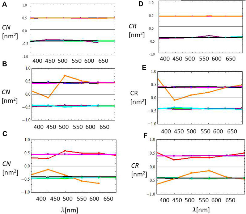
FIGURE 13. (A) to (F) Normalized convolution (CN) and correlation (CR) between wavelength (λ) and measured Zernike coefficients (P_s). Left column: CN [nm²], (A) circular aperture (a = b = 1.7 cm), (B) elliptic aperture 1 (a = 1.5 cm, b = 1.7 cm), and (C) elliptic aperture 2 (a = 1.3 cm, b = 1.7 cm). Right column: CR [nm²], (D) circular aperture (a = b = 1.7 cm), (E) elliptic aperture 1 (a = 1.5 cm, b = 1.7 cm), and (F) elliptic aperture 2 (a =1.3 cm, b = 1.7 cm). Further details are in the text.

5 Discussion

We have presented a comprehensive numerical and experimental study of the spectral response of optical aberrations in macroscopic fluidic lenses with high dioptric power, tunable focal distance, and aperture shape [7]. Our investigation is based on an empirical characterization of the optical and material properties of thin elastic membranes, in particular of the refractive index of polymers, such as PDMS, according to the first-order Sellmeier model [10]. Using a Shack–Hartmann wavefront sensor, we experimentally reconstructed the near-field wavefront transmitted by such fluidic lenses, and we characterized the chromatic response of optical aberrations in terms of Zernike polynomials over the visible wavelength range (λ = 400–650 nm) using an incoherent programmable LED source. Moreover, we further classified the spectral response of the lenses using clustering techniques, encountering that for a predetermined number of clusters (N = 2, 4, 6), the Zernike coefficients characterizing the spectral response can be classified in three main clusters over the entire wavelength range: a cluster with positive Zernike coefficients, a cluster with negative Zernike coefficients, and a cluster with nearly vanishing Zernike coefficients. In addition, we performed correlation (CR) and convolution (CN) measurements, finding that as a general trend Zernike polynomials display either a positive correlation with λ (CR/CN = +0.5) or a negative correlation with λ (CR/CN = −0.5). Fluctuations on this trend increase as the asymmetry in the ellipse axes increases. Experimental results are in agreement with our theoretical model of the nonlinear elastic membrane deformation. A complete characterization of the spectral response of optical aberrations for coherent illumination will be presented in an upcoming work.

Data availability statement

The raw data and numerical codes supporting the conclusions of this article will be made available by the authors upon request, without undue reservation.

Author contributions

GP: conceptualization, construction of experimental setups, data acquisition, data curation, analysis, funding acquisition, investigation, methodology, project administration, resources, validation, writing, review and editing. FM: conceptualization, formal analysis, methodology, theoretical model, software, visualization, and writing.

Funding

The author(s) declare financial support was received for the research, authorship, and/or publication of this article. The authors declare financial support from PICT STARTUP 0710 2015 for the construction of the Shack-Hartmann Wave Front Sensor.

Acknowledgments

The authors are grateful to the Solar Energy Department (TANDAR-CNEA) and to the Laboratory of Polymers (FCEN-UBA) for assistance in PDMS membrane preparation. GP gratefully acknowledges financial support from PICT2014-1543, PICT2015-0710 Startup, UBACyT PDE 2016, and UBACyT PDE 2017.

Conflict of interest

The authors declare that the research was conducted in the absence of any commercial or financial relationships that could be construed as a potential conflict of interest.

The author(s) declared that they were an editorial board member of Frontiers, at the time of submission. This had no impact on the peer review process and the final decision.

Publisher’s note

All claims expressed in this article are solely those of the authors and do not necessarily represent those of their affiliated organizations, or those of the publisher, the editors, and the reviewers. Any product that may be evaluated in this article, or claim that may be made by its manufacturer, is not guaranteed or endorsed by the publisher.

References

1. Goss DA, West RW. Introduction to the optics of the eye. Butterworth-Hienemann (2001).

Google Scholar

2. Keating MP. Geometric, ”physical and visual optics”. Butterworth-Hienemann (2002).

Google Scholar

3. Tasman W, Jaeger EA. Duane’s ophtalmology. LLW (2013).

Google Scholar

4. Callina T, Reynolds TP. Traditional methods for the treatment of presbyopia: spectacles, contact lenses, bifocal contact lenses. Ophthalmol Clin North Am (2006) 19:25–33. doi:10.1016/j.ohc.2005.09.006

PubMed Abstract | CrossRef Full Text | Google Scholar

5. Patent Application WO2006011937A2. Fluidic adaptive lens (2006).

Google Scholar

6. Hazan N, Banerjee A, Kim H, Mastrangelo C. Tunable-focus lens for adaptive eyeglasses. Opt Express (2017) 25:1221. doi:10.1364/oe.25.001221

PubMed Abstract | CrossRef Full Text | Google Scholar

7. Takayama O, Minotti F, Puentes G. Tunable fluidic lenses with high dioptric power. OSA Continuum (2018) 1:181. doi:10.1364/osac.1.000181

CrossRef Full Text | Google Scholar

8. Puentes G, Voigt D, Aiello A, Woerdman JP. Experimental observation of universality in depolarized light scattering. Opt Lett (2005) 30:3216–9. doi:10.1364/ol.30.003216

PubMed Abstract | CrossRef Full Text | Google Scholar

9. G. Puentes Invention Disclosure Nr.20170102760. Adaptive fluidic lenses for subnormal vision segment (2023). (TCPind0335-01).

Google Scholar

10. Schneider F, Draheim J, Kamberger R, Wallrabe U. Process and material properties of polydimethylsiloxane (PDMS) for Optical MEMS. Sensor and Actuators A (2006) 151:95–9. doi:10.1016/j.sna.2009.01.026

CrossRef Full Text | Google Scholar

11. Vallet M, Berge B, Vovelle L. Electrowetting of water and aqueos solutions on poly-ethilene-terephthalate insulating films. Polymer (1996) 37:2465–70.

CrossRef Full Text | Google Scholar

12. Krupenking T, Yang S, Mach P. Tunable liquid microlens. Appl Phys Lett (2003) 82:316–8.

CrossRef Full Text | Google Scholar

13. Kuiper andB S, Hendriks H. Variable-focus liquid lens for miniature cameras. Appl Phys Lett (2004) 85:1128–30. doi:10.1063/1.1779954

CrossRef Full Text | Google Scholar

14. Knollman GC, Bellini JL, Weaver JL. Variable-focus liquid-filled hydroacoustic lens. J Acoust Soc Am (1971) 49:253–61.

CrossRef Full Text | Google Scholar

15. Sigiura N, Morita S. Variable-docus liquid-filled optics lens. App Opt (1993) 32:4181–6. doi:10.1364/AO.32.004181

CrossRef Full Text | Google Scholar

16. Zhang DY, Lien V, Berdichevsky Y, Choi J, Lo YH. Fluidic adaptivelens with high focal length tenability. App Phys Lett (2003) 82:3171–2. doi:10.1063/1.1573337

CrossRef Full Text | Google Scholar

17. Joeng KH, Liu GL, Chronis N, Lee LP. Tunable microdoublet lens array. Opt Express (2004) 12:2494–500. doi:10.1364/opex.12.002494

PubMed Abstract | CrossRef Full Text | Google Scholar

18. Chen J, Wang W, Fang J, Varahramyan K. Variable focusing microlens with microfluidic chip. J Micromech Microeng (2004) 14:675–80. doi:10.1088/0960-1317/14/5/003

CrossRef Full Text | Google Scholar

19. Chronis N, Liu GL, Jeong KH, Lee LP. Tunable liquid-filled microlens array integrated with microfluidic network. Opt Express (2003) 11:2370–8. doi:10.1364/oe.11.002370

PubMed Abstract | CrossRef Full Text | Google Scholar

20. Moran PM, Dharmatilleke s., Khaw AH, Tan KW, Chan ML, Rodriguez I. Fluidic lenses with variable focal length. App Phys Lett (2006) 88:041120. doi:10.1063/1.2168245

CrossRef Full Text | Google Scholar

21. Ren H, Wu S-T. Variable-focus liquid lens. Opt Express (2007) 15:5931–6. doi:10.1364/oe.15.005931

PubMed Abstract | CrossRef Full Text | Google Scholar

22. Polson NA, Hayes MA. Microfluidics: controlling fluids in small places. Anal Chem (2001) 73:312A–319A. doi:10.1021/ac0124585

PubMed Abstract | CrossRef Full Text | Google Scholar

23. Hetch E. Optics. 2nd ed. NY: Addison Wesley (2002).

Google Scholar

24. Beger HM. A new approach to the analysis of large deflections of plates. J Appl Mech (1955) 22:465–72. doi:10.1115/1.4011138

CrossRef Full Text | Google Scholar

25. Mazumdar J. A method for solving problems of elastic plates of arbitrary shape. J Aust Math Soc (1970) XI:95–112. doi:10.1017/s1446788700006030

CrossRef Full Text | Google Scholar

26. Mazumdar J, Jones R. A simplified approach to the analysis of large deflections of plates. J Appl Mech (1974) 41:523–4. doi:10.1115/1.3423325

CrossRef Full Text | Google Scholar

27. Fluidic Lenses Data. Raw experimental data and numerical simulations are availble at our Github repository (2023). Available at: https://github.com/grapts/Fluidic-Lenses-Data. (Accessed 11 August 2023)

Google Scholar