Estimation of ocean turbulence intensity using convolutional neural networks

Understanding the transmission of light in ocean turbulence is of great significance for underwater communication, underwater detection, and other fields. The properties of ocean turbulence can affect the transmission characteristics of light beams, therefore it is essential to estimate the ocean turbulence intensity (OTI). In this study, we propose a deep learning-based method for predicting the OTI. Using phase screens to simulate ocean turbulence, we constructed a database of distorted Gaussian beams generated by Gaussian beams passing through ocean turbulence with varying intensities. We built a convolutional neural network and trained it using this database. For the trained network, inputting a distorted beam can accurately predict the corresponding intensity of ocean turbulence. We also compared our designed network with traditional network models such as AlexNet, VGG16, and Xception, and the results showed that our designed network had higher accuracy.

1 Introduction

Optical signal transmission through seawater is subject to the effects of ocean turbulence, which can cause image blurring, light energy dispersion, and limited resolution at the receiver side in ocean detection and signal transmission [1–4]. In 1976, Fleck first employed the “multi-phase screen method” to simulate the impact of atmospheric turbulence on transmitted beams in free space [5]. The proposal of this model has attached much attention [6–10]. In 2000, Nikishov proposed a spatial power spectrum that incorporates fluctuations in seawater temperature, salinity, and refractive index to describe ocean turbulence, which facilitates a comprehensive examination of the influence of seawater as a medium for laser beam transmission [11]. To date, researchers have explored the propagation property of light beams on propagation in ocean turbulence [12, 13]. For example, Yahya Baykal evaluated the scintillation index of spherical waves in strongly turbulent oceanic environments [12]. These studies revealed that the propagation characterization of a light beam in ocean turbulence depends on the property of underwater turbulence, including the rate of dissipation of kinetic energy per unit mass of fluid, the rate of dissipation of mean-squared temperature, and the ratio of temperature to salinity contributions to the refractive index spectrum, etc. Therefore, estimating these parameters of ocean turbulence is of paramount significance for enhancing the performance and efficiency of underwater communication, detection, scientific research, and engineering applications.

Atmospheric and oceanic turbulence are two common types of turbulence that show similar characteristics, such as causing degradation of light intensity distribution. The refractive index structure constant C2 n is the most critical parameter for describing atmospheric turbulence, and numerous methods have been proposed for evaluating it. For instance, Wang et al. employed an artificial neural network with meteorological parameters, such as temperature and relative humidity, as inputs to estimate refractive index structure constant over the sea surface near Mauna Loa [14]. In another study, Ma et al. utilized convolutional neural networks to estimate the refractive index structure constant of atmospheric turbulence and evaluated the effects of transmission distance, beam multiplexing technique, and beam pattern on the estimation accuracy [15]. Compared to atmospheric turbulence, temperature variations primarily induce refractive index changes in the atmospheric medium, whereas in oceanic turbulence, temperature and salinity jointly determine refractive index fluctuations. A comparison of turbulence spatial power spectra [11, 15] reveals that atmospheric turbulence exhibits a unimodal structure, while oceanic turbulence displays a more intricate bimodal structure. Furthermore, research on the transmission characteristics of atmospheric turbulence is relatively mature, whereas investigations into turbulence models and transmission characteristics in oceanic turbulence are still in their early stages. Consequently, evaluating the parameters of ocean turbulence from the transmission and evolution characteristics of a light beam poses a greater challenge.

In recent years, the advent of deep learning technologies has facilitated rapid advancements in various fields [16–20]. In this study, we propose a convolutional neural network (CNN) for estimating turbulence intensity from the distorted intensity pattern formed by a Gaussian beam through oceanic turbulence, and investigate the effects of different parameters on the estimation results in detail. The paper is structured as follows: First, we describe the simulation system and numerically simulate the intensity evolution of a Gaussian beam in oceanic turbulence. Then, we propose a lightweight CNN estimation structure and provide a detailed description of its architecture. After sufficient training, the lightweight CNN achieves accurate estimation of the three intensity factors of oceanic turbulence. To demonstrate the performance of the lightweight CNN, we conduct a thorough investigation of the effects of network parameters, turbulence parameters, and the type of training dataset on the identification results, and compare the estimation outcomes with those of other networks. Finally, we summarize the completed work and provide an outlook on its future.

2 Fundamental principle

2.1 Propagation model

To simulate the beam propagation in ocean turbulence, we employed a turbulence spectrum method proposed by Ref. [11], which accounts for the effects of seawater temperature, salinity, and refractive index undulation. This turbulence spectrum model is suitable for isotropic homogeneous seawater media and can accurately describe light transmission behavior in seawater, providing favorable conditions for in-depth study of laser transmission characteristics in seawater media. To establish the ocean turbulence phase screen, we used the phase screen method [5] based on the power spectrum inversion method. The effect of oceanic turbulence on beam transmission is considered equivalent to beam transmission through a series of combinations of a random turbulent phase screen and free space, as shown in Figure 1.

FIGURE 1

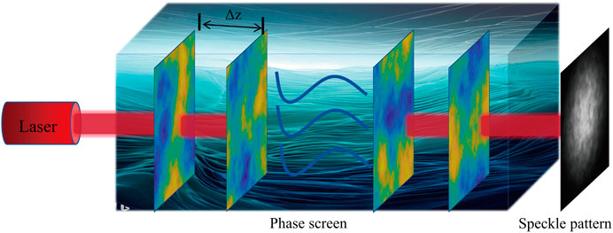
FIGURE 1. Schematic of beam propagation through ocean turbulence.

2.2 Theoretical derivation

The fundamental mode Gaussian beam is selected as the input beam, with the form of:

${\mathbf{U}}_{\mathbf{0}}=\mathbf{exp}\left(-\frac{{\mathit{x}}^{\mathbf{2}}+{\mathbf{y}}^{\mathbf{2}}}{{\mathrm{\omega }}_{\mathbf{0}}}\right)(1)$

where (x, y) is the coordinates of the optical field; ω₀ is the radius of the beam.

The propagation of a laser beam through ocean turbulence is simulated by multi-phase screen, which mimics the effect of turbulence on the beam. At position z_i, the ith phase screen is set, with Δz_i+1 = z_i+1-z_i representing the interval between adjacent phase screens. The propagation of a light field between two consecutive phase screens can be expressed as:

$\mathbf{U}\left(\mathbf{r},{\mathbf{z}}_{\mathbf{i}+\mathbf{1}}\right)={\mathbf{F}}^{-\mathbf{1}}\left\{\mathbf{F}\left\{\mathbf{U}\left(\mathbf{r},{\mathbf{z}}_{\mathbf{i}}\right)\mathbf{exp}\left[\mathbf{i}\mathrm{\phi }\left(\mathbf{x},\mathbf{y}\right)\right]\right\}\times \mathbf{exp}\left(-\mathbf{i}\frac{{\mathbf{k}}_{\mathbf{x}}^{\mathbf{2}}+{\mathbf{k}}_{\mathbf{y}}^{\mathbf{2}}}{\mathbf{2}\mathbf{k}}∆{\mathbf{z}}_{\mathbf{i}+\mathbf{1}}\right)\right\}(2)$

where φ(x, y) is the phase perturbation caused by the phase screens. k_x and k_y are the wave numbers in the x and y directions, k is the wave number in the vacuum. F and F⁻¹ represent the Fourier transform (FT) and the inverse Fourier transform (IFT), respectively. Each phase screen is divided into N×N grids.The matrix of N×N points in the x-y plane represents the optical field, and the total side length of the matrix is L. The range of the matrix is -L/2 < x < L/2, -L/2 < y < L/2.

The following describes how to generate the random phase screen. The phase φ(x, y) is obtained through power spectrum inversion, which involves using the turbulence power spectrum to filter a complex Gaussian random matrix, followed by obtaining the turbulent distortion phase through IFT. This process can be represented as:

$\mathrm{\phi }\left(\mathbf{x},\mathbf{y}\right)=\mathbf{C}{\displaystyle \sum _{{\mathbf{k}}_{\mathbf{x}}}}{\displaystyle \sum _{{\mathbf{k}}_{\mathbf{y}}}}\mathbf{p}\left({\mathbf{k}}_{\mathbf{x}},{\mathbf{k}}_{\mathbf{y}}\right)\sqrt{{\mathbf{F}}_{\mathbf{\Phi }}\left({\mathbf{k}}_{\mathbf{x}},{\mathbf{k}}_{\mathbf{y}}\right)}\mathbf{exp}\left[\mathbf{i}\left(\mathbf{x}{\mathbf{k}}_{\mathbf{x}}+\mathbf{y}{\mathbf{k}}_{\mathbf{y}}\right)\right](3)$

where C is the constant factor that controls the phase screen variance. x = mΔx, y = mΔy, Δx and Δy are the sampling intervals in the spatial domain, m and n are integer. k_x = m′Δk_x, k_y = n′Δk_y, Δk_x and Δk_y are the spatial frequency domain sampling intervals in the wave number domain,m′and n′ are integer. k = 2π/λ is the wave number of the laser. p (k_x, k_y) is the Fourier transform of the Gaussian random number with mean 0 and variance 1. The term F_Φ(k_x, k_y) represents the oceanic phase spectrum on any slice perpendicular to the direction of beam propagation (z-axis), as shown in equation:

${\mathbf{F}}_{\mathbf{\varphi }}\left({\mathbf{k}}_{\mathbf{x}},{\mathbf{k}}_{\mathbf{y}}\right)=\mathbf{2}\mathit{\pi }{\mathit{k}}^{\mathbf{2}}\Delta \mathit{z}\mathit{\varphi }\left({\mathbf{k}}_{\mathbf{x}},{\mathbf{k}}_{\mathbf{y}}\right)(4)$

Φ(k_x, k_y) was calculated based on the refractive index fluctuation spectrum of seawater proposed by Ref. [11], which expression is:

$\mathbf{\varphi }\left({\mathbf{k}}_{\mathbf{x}},{\mathbf{k}}_{\mathbf{y}}\right)=\mathbf{0.388}\times {\mathbf{10}}^{-\mathbf{8}}\times {\left(\sqrt{{\mathbf{k}}_{\mathbf{x}}^{\mathbf{2}}+{\mathbf{k}}_{\mathbf{y}}^{\mathbf{2}}}\right)}^{-\frac{\mathbf{11}}{\mathbf{3}}}{\mathrm{\epsilon }}^{-\frac{\mathbf{1}}{\mathbf{3}}}\left[\mathbf{1}+\mathbf{2.35}{\left(\mathrm{\eta }\sqrt{{\mathbf{k}}_{\mathbf{x}}^{\mathbf{2}}+{\mathbf{k}}_{\mathbf{y}}^{\mathbf{2}}}\right)}^{\frac{\mathbf{2}}{\mathbf{3}}}\right]\times \frac{{\mathbf{X}}_{\mathbf{T}}}{{\mathrm{\omega }}^{\mathbf{2}}}\left[{\mathrm{\omega }}^{\mathbf{2}}{\mathbf{e}}^{\left(-{\mathbf{A}}_{\mathbf{T}}{\mathbf{\sigma }}_{\mathbf{TS}}\right)}+{\mathbf{e}}^{\left(-{\mathbf{A}}_{\mathbf{S}}{\mathbf{\sigma }}_{\mathbf{TS}}\right)}-\mathbf{2}\mathrm{\omega }{\mathbf{e}}^{\left(-{\mathbf{A}}_{\mathbf{TS}}{\mathbf{\sigma }}_{\mathbf{TS}}\right)}\right](5)$

where η is the Kolmogorov scale with the value range is 6 × 10⁻⁵∼10^–2 m. ε is the turbulent kinetic energy dissipation rate per unit volume of seawater, X_T is the mean square temperature dissipation rate. The parameter ω corresponds to the ratio of temperature gradient to salinity gradient, with a range between −5 and 0. As ω approaches 0, it characterizes salinity dominated turbulence, while nearing −5 signifies temperature-dominated turbulence. The negative sign indicates that with increasing seawater depth, there is a decrease in temperature and an increase in salinity. Other parameters are described as follows: A_T = 1.863 × 10⁻², A_S = 1.9 × 10⁻⁴, A_TS = 9.41 × 10⁻³, σ_TS = 8.284 (κη)^4/3 + 12.987 (κη)². The parameters in simulation are set as in Table 1.

TABLE 1

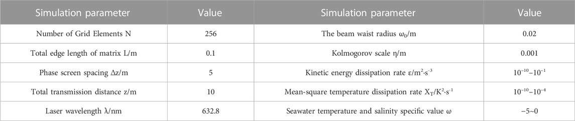
TABLE 1. Parameter of simulation.

3 OTI-CNN network model

To accurately estimate the OTI from distorted patterns, we developed a convolutional neural network called OTI-CNN, as illustrated in Figure 2. The OTI-CNN model was trained using supervised learning with dataset, enabling it to directly predict the parameters of OTI from the input distorted Gaussian beam. The OTI-CNN model comprises seven convolutional layers and two fully connected layers. To prevent information loss in the distorted patterns that may be caused by maximum pooling layers, we set the step size of the convolutional layers to 2 instead, allowing the high-dimensional channels to cover more input features while increasing the network depth.

FIGURE 2

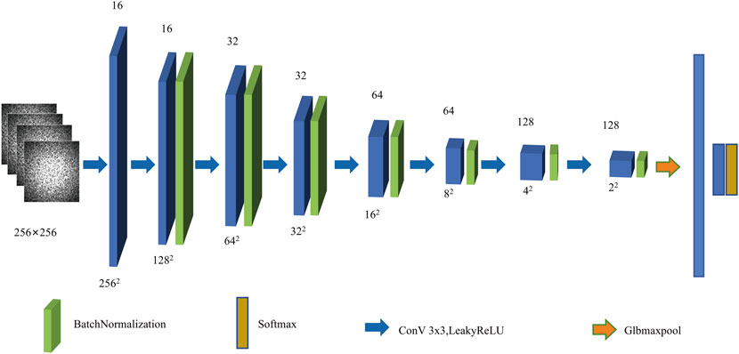
FIGURE 2. Structure diagram of OTI-CNN for estimating ocean turbulence intensity parameters.

The input to the network is a distorted pattern with a size of 256 × 256 pixels. After the first convolutional layer, the network generates 16 feature maps with a size of 256 × 256 pixels. After the second convolutional layer, 16 feature maps with a size of 128 × 128 pixels are generated. The eighth convolutional layer produces a tensor with a size of 2 × 2×128. It flows into the global maxpooling layer [21] and enters the fully connected layer (Dropout rate = 0.3). Finally, using Softmax as the activation function, the output of the network is derived from the fully connected layer, representing the OTI estimate. All convolutional kernels in the OTI-CNN model are of size 3 × 3. After the convolutional layers, we have added a LeakyReLU activation function with an alpha value of 0.2 and a batch normalization layer with a momentum of 0.95 to improve the network’s performance.

The batch size of the network training was set to 16, and the training dataset was split into three parts: training set, validation set, and test set, with a ratio of 8:1:1. The validation and test sets, which were not involved in the training process, were randomly selected from the entire dataset. The network was trained using Python 3.7.13, TensorFlow-gpu 2.4.1, Keras 2.4.3, and a GPU (NVIDIA GeForce RTX 3060 Laptop GPU). We trained the network for 50 epochs and used binary cross-entropy as the loss function. The Adam optimizer [22] was chosen with an initial learning rate of 2 × 10⁻⁴, which was reduced by a factor of 10 at the 20th and 35th epochs.

To measure the recognition ability of OTI-CNN, we defined the accuracy as:

$\mathbf{A}\mathbf{c}\mathbf{c}\mathbf{u}\mathbf{r}\mathbf{a}\mathbf{c}\mathbf{y}=\frac{{\mathbf{y}}_{\mathbf{pred}}}{{\mathbf{y}}_{\mathbf{p}\mathbf{r}\mathbf{e}\mathbf{d}\_\mathbf{a}\mathbf{l}\mathbf{l}}}(6)$

where y_{pred_all} denotes the number of all the predictions, and y_pred denotes the number of the correct predictions.

4 Results and analysis

When a Gaussian beam propagates through seawater, it experiences turbulent perturbations and distortions, resulting in a speckle pattern that contains turbulence information at the output. We use the OTI-CNN model to extract turbulence intensity features from the speckle pattern and estimate the OTI parameters. We discuss the OTI in five groups, named Set 1–5, as shown in Table 2. The variation of OTI is mainly exemplified by temperature and salinity in the ocean, which are represented by the three turbulence intensity parameters: $\mathrm{\epsilon }$, ω and X_T. The parameter $\mathrm{\epsilon }$ represents the turbulent kinetic energy dissipation rate per unit volume of seawater, X_T represents the mean square temperature dissipation rate, and ω represents the ratio of seawater temperature to salinity in the power spectrum.

TABLE 2

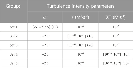
TABLE 2. Parameter setting for ocean turbulence.

Studies have shown [11–13] that the parameter ω varies from −5 to 0 in the marine environment. As ω approaches 0, it indicates that temperature predominantly influences turbulence, while near −5, salinity has a more pronounced impact. It is noteworthy that salinity-dominated turbulence significantly affects the transmission characteristics of optical beams. Additionally, when X_T is large, ε is small, or ω is high, oceanic turbulence has a more pronounced impact on optical beam transmission. Conversely, when X_T is small, ε is large, or ω is low, the effect of oceanic turbulence on beam transmission is reduced. In each experimental Set, we uniformly sample one intensity parameter within the specified range while appropriately setting the other two parameters. This approach ensures a comprehensive estimation of oceanic turbulence parameters while maintaining experimental consistency. In Set1, the parameter ω takes values in the range [−5, −2.75], and 10 OTI samples are collected at intervals of 0.25. The values of ε and X_T are fixed at 10^–6 m² s^-3 and 10^–7 K² s^–1, respectively. For Set 2 and Set 3, ε varies within the range of [10^–10, 10^–1], and 10 and 20 OTI samples are taken with intervals of 10 and 10^–0.5, respectively. Meanwhile, the fixed values of ω and X_T are −2.5 and 10^–7 K² s^–1. In Set 4 and Set 5, X_T is sampled within the range of [10^–10, 10^–4], with 10 and 20 equally spaced sample values, respectively. The fixed values of ω and ε are −2.5 and 10⁻⁶ m² s³, respectively.

Four statistics including mean absolute error (EMAE), mean relative error (EMRE), root mean squared variance (ERMSE) and correlation coefficient (R_xy) were selected to quantitatively evaluate the performance of the network. The definitions of these four statistics are [23]:

$\mathbf{E}\mathbf{M}\mathbf{A}\mathbf{E}=\frac{\mathbf{1}}{\mathbf{N}}{\displaystyle \sum _{\mathbf{I}=\mathbf{1}}^{\mathbf{N}}}{\left({\widehat{\mathbf{y}}}_{\mathbf{i}}-{\mathbf{y}}_{\mathbf{i}}\right)}^{\mathbf{2}}(7)$

$\mathbf{E}\mathbf{M}\mathbf{R}\mathbf{E}={\sum }_{\mathbf{I}=\mathbf{0}}^{\mathbf{N}}\frac{\text{EMAE}}{\left|{\sum }_{\mathbf{I}=\mathbf{0}}^{\mathbf{N}}\frac{{\mathbf{y}}_{\mathbf{i}}}{\mathbf{N}}\right|}(8)$

$\mathbf{E}\mathbf{R}\mathbf{M}\mathbf{S}\mathbf{E}=\sqrt{\frac{\mathbf{1}}{\mathbf{N}}{\sum }_{\mathbf{I}=\mathbf{1}}^{\mathbf{N}}\left({\widehat{\mathbf{y}}}_{\mathbf{i}}-{\mathbf{y}}_{\mathbf{i}}\right)}(9)$

${\mathit{R}}_{\mathit{x}\mathit{y}}=\mathbf{1}-\frac{{\sum }_{\mathit{i}=\mathbf{1}}^{\mathit{N}}{\left({\mathit{y}}_{\mathit{i}}-{\overline{\mathit{y}}}_{\mathit{i}}\right)}^{\mathbf{2}}}{{\sum }_{\mathit{i}=\mathbf{1}}^{\mathit{N}}{\left({\mathit{y}}_{\mathit{i}}-{\widehat{\mathit{y}}}_{\mathit{i}}\right)}^{\mathbf{2}}}(10)$

where N is the total number of test samples; ŷ = {ŷ₁, ŷ₂, ⋯ŷ_n-1, ŷ_n} is the estimated value; y = {y₁, y₂, ⋯y_n-1, y_n} is the true value; $\overline{y}$ is the average value of y_i.

4.1 Intensity estimation for training repetitive speckle patterns

In developing the power spectrum inversion method for ocean turbulence modeling, we generate the phase screen by filtering the power spectrum function of the ocean turbulence phase with a complex Gaussian random matrix. Even when the turbulence intensity parameters remain invariant, the dynamic random variation of the complex Gaussian random matrix can introduce randomness to the turbulence phase screen, resulting in non-negligible variations in the distorted patterns. As a result, when distorted patterns with the same parameters are input to the OTI-CNN, the extracted features may not be exactly the same. It is necessary to investigate the relationship between the number of training samples and estimation accuracy under the same parameters.

We selected Set2 and Set5 as examples to examine the effects of number of the training sample on the performance of the network. The dataset was randomly divided into training, validation, and test sets in an 8:1:1 ratio. The results of the test set were evaluated using four estimation functions (EMAE, EMRE, ERMSE, and R_xy).

Figure 3A illustrates the results of the three estimation error functions (EMAE, EMRE, and ERMSE) for Set2 and Set5 with different number of samples. All of them show a general decreasing trend as the number of samples increases from 100 to 800, indicating that the estimation accuracy improves with an increasing number of replicate samples. Figure 3B presents the variation in correlation coefficients (R_xy) of Set2 and Set5 as the number of sample replicates changes. As the number of duplicate samples increases, the correlation coefficients R_xy of Set2 and Set5 demonstrate an overall upward trend. However, the increasing trend becomes less pronounced when the number of duplicate samples reaches 800. These results validate that increasing the number of training samples is an effective way to improve the performance of the network.

FIGURE 3

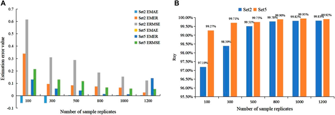
FIGURE 3. Schematic diagram of the relationship between training samples and estimation accuracy. (A) Is the result of three estimation error functions (EMAE, EMER, and ERMSE) for Set2 and Set5. (B) Is the result of the correlation coefficient (Rxy) of Set2 and Set5 transformed with the number of sample replicates.

4.2 Estimation of ocean turbulence intensity from speckle patterns

Table 2 divides the OTI into five control groups (Set1-5), with each group having a replicate sample size of 800 for each parameter. The data sets for Set 1, Set 2, and Set 4 consist of 8000 samples, while the data sets for Set 3 and Set 5 consist of 16000 samples. We split the data with an 8:1:1 ratio to create the training set, validation set, and test set. Figure 4A shows the variation of the accuracy function with training cycles. After 50 training cycles, Set1 achieves an accuracy of 65.9% in ω estimation, while Sets 2 and 3 achieve accuracy levels of 95.6% and 79.8% for ε estimation, respectively. For X_T estimation, Sets 4 and 5 achieve accuracy of 100% and 94.5%, respectively. These results indicate the feasibility of estimating the intensity parameters of the ocean turbulence index (OTI) from the scattering pattern. Furthermore, the identification accuracy of ω has consistently been lower than that of X_T and ε. This is because ω is sampled ten times within the range of −5 to −2.75 with an interval of 0.25. This leads to a lack of distinct features in the distorted Gaussian beam patterns between two adjacent values of ω. When ω takes on values of −5, −4.75, and −4.5, it results in a significant increase in turbulence intensity, which in turn reduces the overall identification accuracy of ω. Figure 4B shows the variation of the loss function with training cycles. The loss function decreases rapidly in the initial training cycles, indicating that the effectiveness of network.

FIGURE 4

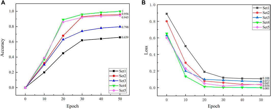
FIGURE 4. Results of 4 statistics for different values of turbulence intensity. (A) The accuracy variation of Set (1–5) with training cycles. (B) The loss function of Set (1–5) with training cycles.

4.3 OTI-CNN model estimation performance improvement and comparison

To validate the advantages of lightweight convolutional neural network-based methods in estimating the intensity of ocean turbulence, we compared the performance of different networks (AlexNet, VGG16, and Xception) in estimating the parameter X_T. We selected Set 5 and collected 800 sample values repeatedly for each OTI value.

The AlexNet model [24] comprises 5 convolutional layers, 3 fully connected layers, and 1 softmax layer. The VGG16 model [25] is composed of 13 convolutional layers, 3 fully connected layers, and 1 softmax layer. VGG16 differs from AlexNet in that it replaces the 7 × 7 sized convolutional kernels with multiple 3 × 3 sized convolutional kernels, which better preserves the image’s nature, increase network depth while maintaining the same perceptual field, and enables the system to learn more complex patterns. In 2014, Christian Szegedy proposed Inception (GoogLeNet) [26], a new deep learning architecture. Before this, AlexNet, VGG, and other structures achieved better training results by increasing the network’s depth (number of layers). However, adding layers came with various negative effects such as overfitting, gradient vanishing, and gradient exploding. Xception [27], an improved version of Inception, achieves complete decoupling of cross-channel correlation and spatial correlation in the feature map of convolutional neural networks. The Xception architecture consists of 36 convolutional layers, organized into 14 modules, with all modules surrounded by linear residual connections except for the first and last modules. Essentially, the Xception architecture is a linear stack of deeply separable convolutional layers with residual connections.

As seen in Section 3, the main body of the OTI-CNN model consists of seven 3 × 3 convolutional layers and an average pooling of two fully connected layers. The OTI-CNN model utilizes 3 × 3 convolutional kernels, avoiding the issue of image feature loss associated with the use of 7 × 7 kernels in the AlexNet model. In comparison to VGG and Xception, the OTI-CNN network architecture is designed to be lightweight, effectively mitigating problems such as overfitting, gradient vanishing, and gradient explosion that can arise from increasing network depth. Additionally, we have incorporated convolutional layers with a stride of 2 to replace the max-pooling layers in VGG. This enables high-dimensional channels to cover more input features while deepening the network.

Table 3 presents the estimation results. The OTI-CNN model exhibits relatively good estimation performance, considering both the estimation results of the test set and the training time. Wang et al. demonstrated that cropped speckle patterns also contain most of the feature information [28]. In practice, to achieve a lightweight effect, we can input a 32 × 32 or 64 × 64 scatter pattern to further speed up the neural network and reduce hardware usage.

TABLE 3

TABLE 3. Parameter setting for ocean turbulence.

5 Conclusion

In conclusion, we have demonstrated the potential of using a deep learning-based method to estimate the parameters of ocean turbulence. By employing the power spectrum inversion method, we simulated the distorted intensity patterns of a laser beam propagating through ocean turbulence. We designed an OTI-CNN network and trained it with the distorted intensity patterns. Our results show that the designed OTI-CNN model can accurately estimate the parameters X_T, ω, and ε related to the intensity of ocean turbulence. For a single parameter sample with a repeated speckle pattern number of 800, the accuracy of OTI-CNN can reach 65.9% for estimating ω, up to 95.6% for estimating ε, and up to 100% for estimating X_T. We also investigated the impact of the number of samples on the estimation accuracy. The results indicated that increasing the number of samples is an effective way to improve the network’s performance. Furthermore, we compared the OTI-CNN model with other models, namely, AlexNet, VGG16, ResNet18, and Xception, and found that the OTI-CNN model outperformed the other models in terms of overall estimation performance.

Data availability statement

The original contributions presented in the study are included in the article/Supplementary Material, further inquiries can be directed to the corresponding authors.

Author contributions

YC: Conceptualization, Data curation, Formal Analysis, Investigation, Methodology, Software, Writing–original draft. XL: Resources, Supervision, Funding acquisition, Writing–review and editing. JJ: Data curation, Writing–review and editing. SG: Formal Analysis, Writing–review and editing. YL: Software, Writing–review and editing. YJ: Funding acquisition, Writing–review and editing.

Funding

The authors declare financial support was received for the research, authorship, and/or publication of this article. This work was supported by the Scientific Research Fund of the Liaoning Provincial Education Department (No. LJKMZ20220620) and the 2023 Central Government guidance for local science and technology development funds (basic research of free exploration) (No. 2023JH6/100100066).

Conflict of interest

The authors declare that the research was conducted in the absence of any commercial or financial relationships that could be construed as a potential conflict of interest.

Publisher’s note

All claims expressed in this article are solely those of the authors and do not necessarily represent those of their affiliated organizations, or those of the publisher, the editors and the reviewers. Any product that may be evaluated in this article, or claim that may be made by its manufacturer, is not guaranteed or endorsed by the publisher.

References

1. Dubreuil M, Delrot P, Leonard I, Alfalou A, Brosseau C, Dogariu A. Exploring underwater target detection by imaging polarimetry and correlation techniques. Appl Opt (2013) 52(5):997–1005. doi:10.1364/ao.52.000997

PubMed Abstract | CrossRef Full Text | Google Scholar

2. Kocak DM, Dalgleish FR, Caimi FM, Schechner YY. A focus on recent developments and trends in underwater imaging. MAR TECHNOL SOC J (2018) 42(1):52–67. doi:10.4031/002533208786861209

CrossRef Full Text | Google Scholar

3. Kaushal H, Kaddoum G. Underwater optical wireless communication. IEEE Access (2016) 4:1518–47. doi:10.1109/access.2016.2552538

CrossRef Full Text | Google Scholar

4. Arnon S. Underwater optical wireless communication network. Opt Eng (2010) 49(1):015001. doi:10.1117/1.3280288

CrossRef Full Text | Google Scholar

5. Fleck JA, Morris JR, Feit MD. Time-dependent propagation of high energy laser beams through the atmosphere. Appl Phys (1976) 10(2):129–60. doi:10.1007/bf00896333

CrossRef Full Text | Google Scholar

6. Hill RJ. Optical propagation in turbulent water. J Opt Soc Am (1978) 68(8):1067–72. doi:10.1364/josa.68.001067

CrossRef Full Text | Google Scholar

7. Dillon TM. The energetics of overturning structures: Implications for the theory of fossil turbulence. J Phys Oceanogr (1984) 14(3):541–9. doi:10.1175/1520-0485(1984)014<0541:teoosi>2.0.co;2

CrossRef Full Text | Google Scholar

8. Gargett AE. Vertical eddy diffusivity in the ocean interior. J MAR RES (1984) 42(2):359–93. doi:10.1357/002224084788502756

CrossRef Full Text | Google Scholar

9. Gargett AE, Holloway G. Sensitivity of the GFDL ocean model to different diffusivities for heat and salt. J Phys Oceanogr (1922) 22(10):1158–77. doi:10.1175/1520-0485(1992)022<1158:sotgom>2.0.co;2

CrossRef Full Text | Google Scholar

10. Cheng Y, Canuto VM. Stably stratified shear turbulence: A new model for the energy dissipation length scale. J Atmos Sci (1994) 51(16):2384–96. doi:10.1175/1520-0469(1994)051<2384:ssstan>2.0.co;2

CrossRef Full Text | Google Scholar

11. Nikishov VV, Nikishov VI. Spectrum of turbulent fluctuations of the sea-water refraction index. Int J Fluid Mech Res (2000) 27(1):82–98. doi:10.1615/InterJFluidMechRes.v27.i1.70

CrossRef Full Text | Google Scholar

12. Baykal Y. Scintillation index in strong oceanic turbulence. Opt Commun (2016) 375:15–8. doi:10.1016/j.optcom.2016.05.002

CrossRef Full Text | Google Scholar

13. Pan S, Wang L, Wang W, Zhao S. Author correction: An effective way for simulating oceanic turbulence channel on the beam carrying orbital angular momentum. Sci Rep (2020) 10(1):1268. doi:10.1038/s41598-020-58156-7

PubMed Abstract | CrossRef Full Text | Google Scholar

14. Yao W, Sukanta B. Using an artificial neural network approach to estimate surface-layer optical turbulence at Mauna Loa, Hawaii. Opt Lett (2016) 41(10):2334–7. doi:10.1364/OL.41.002334

PubMed Abstract | CrossRef Full Text | Google Scholar

15. Ma S, Hao S, Zhao Q, Xu C. “Estimation of atmospheric turbulence intensity based on deep learning,” in Proc. SPIE 11907, Sixteenth National Conference on Laser Technology and Optoelectronics (2021), 1190726. doi:10.1117/12.2603106

CrossRef Full Text | Google Scholar

16. Shi C, Tan C, Wang T, Wang L. A waste classification method based on a multilayer hybrid convolution neural network. Appl Sci (2021) 11(18):8572. doi:10.3390/APP11188572

CrossRef Full Text | Google Scholar

17. Topple JM, Fawcett JA. MiNet: Efficient deep learning automatic target recognition for small autonomous vehicles. IEEE Geosci Remote Sens Lett (2020) 18(06):1014–8. doi:10.1109/lgrs.2020.2993652

CrossRef Full Text | Google Scholar

18. Dong Y, Pan B. A review of speckle pattern fabrication and assessment for digital image correlation. Exp Mech (2017) 57:1161–81. doi:10.1007/s11340-017-0283-1

CrossRef Full Text | Google Scholar

19. Guo G, Zhang N. A survey on deep learning based face recognition. Comput Vis Image Underst (2019) 189(C):102805. doi:10.1016/j.cviu.2019.102805

CrossRef Full Text | Google Scholar

20. Zaid A, Bo P, Ali NRA, Al-antari MA, Al-Jarazi R, Zhai D. A hybrid deep learning pavement crack semantic segmentation. Eng Appl Artif Intell (2023) 122:106142. doi:10.1016/J.ENGAPPAI.2023.106142

CrossRef Full Text | Google Scholar

21. Zhou B, Khosla A, Lapedriza À, Oliva A, Torralba A. Learning deep features for discriminative localization (2015). Avaialble at: https://arxiv.org/abs/1512.04150.

Google Scholar

22. LeCun Y, Bottou L, Bengio Y, Haffner P. Gradient-based learning applied to document recognition. Proc IEEE Inst Electr Electron Eng (1998) 86(11):2278–324. doi:10.1109/5.726791

CrossRef Full Text | Google Scholar

23. Gao S, Liu X, Chen Y, Jiang J, Liu Y, Jiang Y, et al. Atmospheric turbulence strength estimation using convolution neural network. IEEE Photon. J. (2023). doi:10.1109/JPHOT.2023.3314833

CrossRef Full Text | Google Scholar

24. Krizhevsky A, Sutskever I, Hinton EG. ImageNet classification with deep convolutional neural networks. Commun ACM (2017) 60(6):84–90. doi:10.1145/3065386

CrossRef Full Text | Google Scholar

25. Simonyan K, Zisserman A. Very deep convolutional networks for large-scale image recognition (2014). Avaialble at: https://arxiv.org/abs/1409.1556.

Google Scholar

26. Szegedy C, Liu W, Jia Y, Sermanet P, Reed S, Anguelov D, et al. Going deeper with convolutions (2014). Avaialble at: https://arxiv.org/abs/1409.4842.

Google Scholar

27. Wazir M, Supavadee A, Takao O. Multi-scale Xception based depthwise separable convolution for single image super-resolution. PloS one (2021) 16(8):e0249278. doi:10.1371/JOURNAL.PONE.0249278

PubMed Abstract | CrossRef Full Text | Google Scholar

28. Wang Z, Lai X, Huang H, Wang X, Li H, Chen Z, et al. Recognizing the orbital angular momentum (OAM) of vortex beams from speckle patterns. Sci China Phys Mech Astron (2022) 65(4):244211. doi:10.1007/S11433-021-1849-3

CrossRef Full Text | Google Scholar