Modeling of the high-resolution optical-coherence diagnostics of bi-refringent biological tissues

We present a computer model of the polarization-sensitive interference diagnostics of the bi-refringent biological media, with a particular example of the lamella of eye cornea. The diagnostic procedure employs the modified Mach–Zehnder interferometer with controllable phase retardation of the reference wave, separate observation of the orthogonal linearly-polarized interference signals, and evaluation of the phases and amplitudes of their variable (AC) components. The data obtained permit to determine the mean refractive index as well as the difference between the extraordinary and ordinary refractive indices, which, in turn, indicates the optical axis and the collagen fibers’ orientation in the lamella. The modelled procedure enables the sample structure diagnostics with the longitudinal and lateral resolution ∼100 nm and ∼1.8 μm, correspondingly. In particular, it permits a reliable detection and quantitative characterization of a thin (<100 nm) near-surface layer where the mean refractive index differs by less than 1% from that in the main volume (due to the different orientation of the collagen fibers). The diagnostic approach, developed in the paper, can be useful in various problems of structure characterization of optically-anisotropic biological tissues.

1 Introduction

In the early 1990s, it was proposed to use the principles of low-coherence interferometry for obtaining tomographic images of biological tissues with high spatial resolution [1, 2]. This approach, known as “optical coherence tomography” (OCT), opened up new horizons in several areas of medical research, in particular in ophthalmology and dermatology [3–5].

The principles of OCT are based on the properties of biological tissues, whose physical features (mechanical and optical density, specific possibilities to absorb and/or scatter the light energy) affect their ability to reflect the light signal. In this context, the portions of light energy reflected by the tissue layers situated at different depths under the sample surface, can be discriminated due to the limited coherence length of the probing radiation: via scanning the phase retardation of the reference wave, one can observe the interference signal formed by the reflected light “originating” from the desirable tissue section.

Based on the same principles that date back to the period when the OCT ideas were first formulated, a lot of special technological solutions were further developed. The main improvements were directed to the search for possibilities of obtaining several adjacent scans along the sample depth and area in order to recover topographic information about the structure of the whole tissue volume [3–5], and to enhancement of the OCT spatial resolution. As a rule, the longitudinal (axial) resolution is determined by the degree of the probing light temporal coherence, while the transverse resolution of the tomographic system is dictated the angular dimensions of the source. With the OCT [1, 2, 6], both the longitudinal and transverse spatial resolution of the image is achieved at levels of 1—15 µm, which is an order of magnitude higher than when using ultrasound.

Nevertheless, wide application of the OCT as a method for tomography of transparent and translucent media by recording the reflected and back-scattered radiation had indicated its shortcomings in the problems of direct differentiation of various specific tissues, their elements, individual layers of an object, especially, in situations where the tissue elements are damaged, displaced or deformed. The limitations can be overcome if the set of measured parameters is expanded. An immediate step in this direction involves, in addition to registering the radiation intensity, the light polarization measurements, thus switching to the polarization sensitive (PS) OCT [7–10]. Additional information, contained in the reflected-light polarization, not only enables to reveal the specific polarization-sensitive properties of the object (especially valuable because biological tissues and elements frequently show a bi-refringent behavior [8, 9]) but also contribute to increasing the contrast and resolution of the “traditional” intensity-dependent images of the samples under study.

There are known several different designs of the PS-OCT setups operating with different input polarization states, different detection schemes, etc. The main differences between a conventional OCT setup and a PS-OCT arrangement are that a light wave with a specific prescribed state of polarization (SOP) (or switchable set of SOPs) must be used to illuminate the sample [11–15], the SOP should be maintained (or controllably changed) during the light passage through the diagnostic system, and at least two separate detection channels are necessary to register the orthogonal polarization components of the tomographic signal.

In particular, the systems, in which multiple SOPs are used, provide the possibility of access to additional polarization quantities. For example, the Stokes vector quantification, Jones matrix characterization, and Müller matrix measurements are implemented for samples in which the birefringence axes (orientations of birefringent fibers) strongly vary with depth, or the probe radiation experiences significant attenuation due to absorption during the beam propagation [14]. In combination with other OCT approaches, the PS-OCT methods lead to increase of the tomography sensitivity, better image contrast and reducing the time necessary for the full longitudinal and transverse sample scanning.

However, the PS-OCT technique is coupled with some limitations stipulated, for example, by the image speckle structure. Traditional PS-OCT schemes meet difficulties in characterization of the specific features inherent in surface and sub-surface regions of the objects. To realize the PS-OCT measurements for a thin near-surface layer (NSL), specific approaches of endoscopic and needle tomography have been developed, which, as a rule, are slightly invasive and are accompanied by some damage to the sample surface [16, 17].

In this paper, we propose and theoretically analyze efficient PS-OCT procedures for sensitive measurements of optical and structure properties of biological birefringent objects with micrometer transverse resolution and sub-micrometer longitudinal resolution. As an example, the lamella of the eye cornea is considered, with the special attention to detection and characterization of the lamella inhomogeneity in the longitudinal direction. In particular, it is shown that the low-coherent PS-OCT approach enables a non-invasive informative characterization of the near-surface distortions of the lamella structure. Combinations of the ellipsometric and interferometric measurements, involving the modified Mach–Zehnder interferometer, with the correlation and amplitude measurements gives additional possibilities for high-sensitive, comprehensive and reliable recovering the sample structure without its mechanical damage or deformation.

2 Structure and properties of a biological birefringent object

As an example of a birefringent biological object, we consider the eye cornea, the main structural element of which is a lamella – the plate containing tightly packed collagen fibers (Figure 1). Depending on the type, the lamellae differ in their sizes from 0.5 to 200 µm in width and from 0.2 to 2.5 µm in thickness [18]. Optical properties of the cornea [6] are characterized by its high transparency to visible and infrared radiation.

FIGURE 1

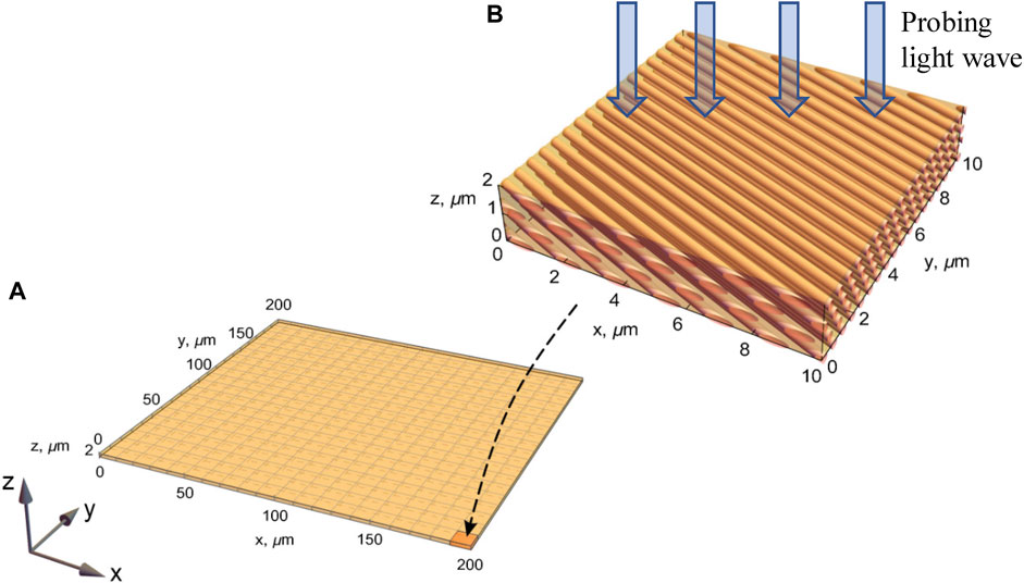
FIGURE 1. Model of the lamella structure accepted for simulations. (A) Schematic lamella plate of the realistic size $200\mu \mathrm{m}\times 200\mu \mathrm{m}\times 2\mu \mathrm{m}$; (B) highlighted and magnified fragment $10\mu \mathrm{m}\times 10\mu \mathrm{m}\times 2\mu \mathrm{m}$ being the subject of investigation. In (B), the collagen fibers are schematically shown with additional 10-fold magnification for better visibility. Their orientation in the (x, y) plane corresponds to $\alpha =-20°$. The probing light (arrows) approaches from the z-direction.

Collagen fibers of the cornea lamellae are characterized by a refractive index n_coll = 1.415; they are surrounded by the base substance medium with a refractive index n_base = 1.356 [19]. The fibers are of cylindrical shape, normally possessing identical diameters, and are oriented parallel to each other and parallel to the lamella plane. The diameter of a collagen fiber is about 30.8 nm, the average distance between them is 55.3 nm [19].

Such a cellular structure implies a possibility of radiation scattering by individual fibers, which would make the lamellae, and the cornea as a whole, opaque. In fact, the cornea is transparent and transmits up to 90% of the incident radiation [20]. According to existing theories [21–23], this is explained by the interference damping of backscattered secondary waves and amplification of forward-scattered ones [20]; the transmission attenuation becomes relevant in the case of the lamella’s waviness, which may appear due to the eye swelling or the cornea edema [24].

In general, each lamella is a birefringent structure, which is characterized by the shape anisotropy [25, 26]. According to the existing model of the eye cornea [25–30], individual lamellae can be considered as uniaxial wave plates, for which the optical axis is oriented parallel to the direction of the collagen fibers (see Figure 1). From lamella to lamella, the optical axes change their orientation within the lamella plane. The predominant optical-axis orientation of the lamellae determines both linear birefringence and absorption dichroism. Introducing the Cartesian frame (x, y) in the lamella plane, we can characterize the local optical-axis position via the angle α between the x-axis and the collagen fibers.

Within the framework of the computer tomography, the lamella is illuminated normally to its plane (see Figure 1), and the radiation transmitted through its thickness and reflected from its back surface carries valuable information relating the lamella’s optical properties and inhomogeneity. According to the above description, a lamella plate can be modeled as a birefringent plate with the optical axis orthogonal to the propagation direction normal to the plate surface (z-direction); the optical-axis orientation within the (x, y) plane is random. In the first approximation, we disregard the presence of scattering centers (keratocytes) localized between the lamellae layers, supposing that the light beam interaction with these centers is insignificant [20–24].

The observed lamella birefringence is a linear shape birefringence, which is positive, since the fibers are contained in a medium with a lower refractive index. The birefringence is characterized by the difference between the ordinary $n_o$ and extraordinary $n_e$ refractive indices [25],

$∆n=\left(n_e-n_o\right)=\frac{\left(n_{\text{coll}}^2-n_{\text{base}}^2\right)\left(n_{\text{coll}}+n_{\text{base}}\right)\nu \left(1-\nu \right)}{\left(1+\nu \right)n_{\text{coll}}^2+\left(1-\nu \right)n_{\text{base}}^2}(1)$

where $\nu$ is the volume content of the collagen fibers. Since $\nu =0.32$ [19], Eq. 1 determines $∆n=0.053$ [25]. The mean refractive index is

$\overline{n}=\left(n_e+n_o\right)/2=\nu n_{\text{coll}}+\left(1-\nu \right)n_{\text{base}}=1.375,(2)$

which dictates

$n_e=1.4015,n_o=1.3485(3)$

in agreement with the literature data [25].

The object of the study – the eye cornea – determines the effective operating wavelength, which is used to simulate the processes of PS-OCT diagnostics. Here, the two aspects should be kept in mind: the good penetration of probing radiation into the tissue under study and the possibility of the sample NSL scanning. In ophthalmic systems, the choice of the wavelength is determined by the need for sufficient penetration of light through the retinal pigment epithelium, for which the wavelengths 850 nm–1,050 nm are appropriate [31].

The choice of the wavelength is related to the bandwidth of the light source to achieve the necessary axial resolution. We consider the radiation of a Ti: Sapphire laser (widely used in ophthalmology) with the central wavelength, corresponding central wavenumber and the spectral width

${\lambda }_0=850\text{\hspace{0.17em}nm},k=0.739\bullet {10}^5{\text{cm}}^{-1},\Delta \lambda =170\text{\hspace{0.17em}nm};(4)$

the power spectrum is supposed to be Gaussian [32],

$\mathrm{S}\left(\lambda \right)\propto \exp \left[-\frac{4\ln 2{\left(\lambda -{\lambda }_0\right)}^2}{{∆\lambda }^2}\right](5)$

($∆\lambda$ has the meaning of “full width at half-maximum” so that $\mathrm{S}\left({\lambda }_0\pm ∆\lambda /2\right)=\left(1/2\right)S\left({\lambda }_0\right)$). Such a choice of the probe wavelength corresponds to the transparency window, limited by the eye cornea absorption bands [33]. The power spectrum (5) determines the coherence length

$l_c=\frac{2\ln 2}{\pi \overline{n}}\bullet \frac{{\lambda }_0^2}{\Delta \lambda }=1.36\mu \mathrm{m}(6)$

where the numerical value corresponds to conditions (3) and (4); it characterizes the longitudinal resolution of the PS-OCT [4, 33].

The lateral resolution [4] is limited by the size of the focused spot, which is determined by the numerical aperture NA of the objective,

$\delta x=\sqrt{2\ln 2}\frac{{\lambda }_0}{\pi \bullet NA}.(7)$

For increasing the lateral resolution, it is tempting to use high-NA objectives; however, another parameter, the depth of focus b (sometimes called as confocal parameter),

$b=\frac{\overline{n}\bullet {\lambda }_0}{2\pi \bullet {NA}^2},$

should be also taken into account. The value of b determines the “penetrating ability” of the longitudinal scanning and must exceed the probed sample thickness. For example, if a cornea thickness is about 500 μm, a numerical aperture NA = 0.02 is required with corresponding lateral resolution ∼16 μm. In eye studies, the lateral resolution 5—15 μm is usual [4]; in our simulations, we accept $NA=0.18$, which dictates the lateral resolution δx ∼ 1.8 μm and b = 5.75 μm (appropriate for the lamella thickness 2 μm).

3 Interferometric PS-OCT diagnostics of the birefringent tissue

A scheme of the model equipment is shown in Figure 2. The Ti: Sapphire laser L produces the x-polarized radiation which enters the Mach-Zehnder interferometer formed by polarization-neutral beam splitters BS1, BS2, BS3 and BS4. The reference arm includes BS2 and the adjustable mirror M that enables to introduce controllable phase retardation of the reference wave; additionally, the half-wave plate HWP can be placed between BS2 and BS4 to switch between the x- and y-polarization state of the reference wave. The sample S of the biological birefringent object (lamella) is placed in the probing arm. The radiation reflected by BS3 is focused on the sample by the objective (not shown in Figure 2), enters the sample and is partially reflected by the front and back sample surfaces. The reflected radiation, whose polarization state is transformed due to the double passage of the sample depth, is again collected by the objective and propagates through BS3 to BS4 where it is superposed with the reference wave. Polarizers Px and Py, selective for the x- and y-polarized components, and the corresponding detectors Dx and Dy, form the x- and y-channels of measurements. The detectors’ signals are compared and processed in the real time. We imply that the wave amplitudes in each arm can be adjusted at any desirable level by means of the standard elements (neutral filters) not shown in Figure 2.

FIGURE 2

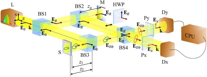
FIGURE 2. Modified Mach–Zehnder scheme for the lamella diagnostics: (L) radiation source, (BS1, BS2, BS3, BS4) beam-splitters, (М) mirror, (HWP) half-wave plate, (S) sample, (Dx, Dy) photodetectors, (CPU) computer unit, (${\mathbf{E}}_0$) incident linearly-polarized beam with x-polarization, (${\mathbf{E}}_R$) reference beam, (${\mathbf{E}}_{Ob}$) object beam, (k) direction of the beam propagation, (${\mathbf{E}}_x$) interference beam formed in the x-channel behind BS4, (${\mathbf{E}}_y$) interference beam formed in the y-channel behind BS4, (Px, Py) polarizers selectively transparent for x- and y-polarized waves.

According to the properties of a biological sample discussed in Section 2, the lamella represents a birefringent uniaxial plate which can be described by the Jones matrix [34, 35].

$M=e^{i\delta }\left(\begin{array}{cc}\cos \frac{\gamma }{2}+i\sin \frac{\gamma }{2}\cos 2\alpha & i\sin \frac{\gamma }{2}\sin 2\alpha \\ i\sin \frac{\gamma }{2}\sin 2\alpha & \cos \frac{\gamma }{2}-i\sin \frac{\gamma }{2}\cos 2\alpha \end{array}\right)(8)$

where $\gamma =k\Delta nd$, $\Delta n=n_e-n_o$ is the difference between the extraordinary and ordinary indices (1), $d=z_1-z_2$ is the sample thickness, $\delta =k\overline{n}d$ is its mean optical thickness, $\overline{n}=\left(n_o+n_e\right)/2$ is the mean refractive index (2), and $\alpha$ is the orientation angle of the sample’s fast axis with respect to the x-axis.

Note that the Jones matrix formalism ignores possible effects of the probing wave depolarization during its propagation inside the sample, and this is a rather common situation for the PS-OCT technique [15]. Generally, depolarization may appear due to multiple scattering or scattering at irregularly shaped inhomogeneities of the near-wavelength size [15] but such events are highly improbable in the lamella samples with thickness of the wavelength range (see the 1st paragraph of Section 2). Therefore, the assumption of negligible depolarization is well justified for the lamella studies and is kept in the present work.

The wave generated by laser L (see Figure 2) is x-polarized; the additional reflection in the BS3 produces the phase jump π, so the probe wave approaching the sample is characterized by the Jones vector ${\mathbf{E}}_0=E_0\left(\begin{array}{c}-1\\ 0\end{array}\right)$ where $E_0$ is the wave amplitude. The object wave contains two parts. The first one appears due to reflection at the sample front surface distanced by z₁, which determines its Jones vector

${\mathbf{E}}_1=\left(\begin{array}{c}{a}_{1x}\exp \left(i{\phi }_{1x}\right)\\ 0\end{array}\right)=E_0{r}_1{e}^{i\pi +2i{kz}_1}\left(\begin{array}{c}-1\\ 0\end{array}\right),(9)$

${\phi }_{1x}=\pi +2k{z}_1,a_{1x}=E_0{r}_1$

Similarly, the second object-wave part emerges upon reflection at the sample back surface and accumulates the changes induced on the double passage through the whole sample thickness:

${\mathbf{E}}_2=\left(\begin{array}{c}{a}_{2x}\exp \left(i{\phi }_{2x}\right)\\ a_{2y}\exp \left(i{\phi }_{2y}\right)\end{array}\right)=M\bullet M\bullet r_2{\left(1-r_1\right)}^2{e}^{2i{kz}_1}{\mathbf{E}}_0$

$=-E_0{r}_2{\left(1-r_1\right)}^2{e}^{2i{kz}_1}{e}^{2i\delta }\left(\begin{array}{c}\cos \gamma +i\sin \gamma \cos 2\alpha \\ i\sin \gamma \sin 2\alpha \end{array}\right)(10)$

where

${\phi }_{2x}=\pi +2k{z}_1+2k\overline{n}d+\arctan \left(\tan \gamma \cos 2\alpha \right),a_{2x}=E_0{r}_2{\left(1-r_1\right)}^2\sqrt{{\cos }^2\gamma +{\sin }^2\gamma {\cos }^{2}2\alpha },$

${\phi }_{2y}=\pi +2k{z}_1+2knd+\pi /2,a_{2y}=E_0{r}_2{\left(1-r_1\right)}^2\left|\sin \gamma \sin 2\alpha \right|.(11)$

Note that in most cases, the front and back lamella surfaces contact the same environmental medium with the refractive index $n_m$, and

$r_1=r_2=\frac{\left|n_m-\overline{n}\right|}{\left|n_m+\overline{n}\right|};(12)$

for example, $n_m=1$ in the usual laboratory situation where the medium is air (it is this situation that is considered in the paper). The total object field is ${\mathbf{E}}_{Ob}={\mathbf{E}}_1+{\mathbf{E}}_2$ (see Figure 2).

In the BS4, the object waves (9) and (10) interfere with the reference wave having passed the BS1 and BS2. Due to the double BS reflection, the corresponding π-jump of the phase vanishes, and the only additional phase is due to the double path z_R (see Figure 2) which serves for controllable reference-wave phase scanning. In the basic mode, the reference wave preserves the initial x-polarization, and

${\mathbf{E}}_R={\mathbf{E}}_{Rx}=A_{Rx}{e}^{2i{kz}_R}\left(\begin{array}{c}1\\ 0\end{array}\right)(\mathrm{13a})$

where $A_{Rx}$ is adjusted to compensate undesirable amplitude disbalances in the reference and object arms of the interferometer (basically $A_{Rx}=E_0$ but in any specific practical situation it is chosen closer to $a_{1x}{,a}_{2x}$ to enable a distinct interference pattern; the results of such adjustment are shown, e.g., in Figures 3, 4). The interference between the object-wave x-components of (9), (10) and the reference wave (6) is observed in the x-channel (Dx, Figure 2). For the study of y-polarized component (10), the y-channel (Dy) is furnished with the y-selective polarizer; simultaneously, the reference wave polarization is transformed to y-oriented by the adjustable half-wave plate (HWP, Figure 2), which gives

${\mathbf{E}}_R={\mathbf{E}}_{Ry}=A_{Ry}{e}^{2i{kz}_R}\left(\begin{array}{c}0\\ 1\end{array}\right)(\mathrm{13b})$

where $A_{Ry}$ can be deliberately adjusted following the same principles as were discussed above for $A_{Rx}$. The interference field has the general form $\mathbf{E}={\mathbf{E}}_R+{\mathbf{E}}_1+{\mathbf{E}}_2$; in the x(y)-channel, ${\mathbf{E}}_R$ is taken in the form (13a) (13b), and the projection of $\mathbf{E}$ onto the x(y)-polarization can be observed [35–37].

FIGURE 3

FIGURE 3. Intensity (18) in the x-channel of the interferometer described by Figure 2 as a function of the reference–object waves’ path difference Δz₁ (15). Yellow line shows the envelopes determined by the coherence function (17) in the last summands of Eq. 18.

FIGURE 4

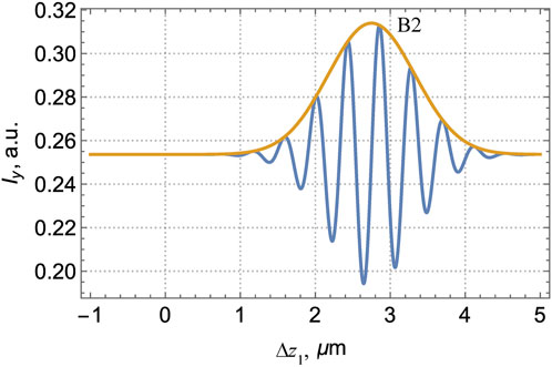
FIGURE 4. Intensity (19) in the y-channel of the interferometer described by Figure 2, as a function of the reference–object waves’ path difference Δz₁ (15). Yellow line is the envelope determined by the coherence function (17) in the last summand of Eq. 19.

Therefore, in the x-channel the intensity $I_x={\left|E_x\right|}^{\mathbf{2}}$ of the interference field is

$I_x=A_{Rx}^2+a_{1x}^2+a_{2x}^2+2A_{Rx}{a}_{1x}\cos \left(2k\Delta z_1-\pi \right)$

$+2A_{Rx}{a}_{2x}\cos \left[2k\Delta z_2-\pi -\arctan \left(\tan \gamma \cos 2\alpha \right)\right](14)$

where

$\Delta z_1=z_R-z_1,\Delta z_2=z_R-z_1-\overline{n}d(15)$

are the optical-path differences for the interfering waves ${\mathbf{E}}_R$ and ${\mathbf{E}}_1$, ${\mathbf{E}}_R$ and ${\mathbf{E}}_2$ (the term responsible for interference between ${\mathbf{E}}_1$ and ${\mathbf{E}}_2$ is supposed to be negligible). Similarly, in the y-channel

$I_y=A_{Ry}^2+a_{2y}^2+2A_{Ry}{a}_{2y}\cos \left(2k\Delta z_2-\pi -\pi /2\right).(16)$

Eqs 14 and (16) suppose the complete coherence of the interfering waves. In practice, the laser source produces a partially coherent radiation with the longitudinal coherence function [3]:

$\mathrm{\Gamma }\left(z\right)=\exp \left(-z^2∆k^2\right)(17)$

where $∆k=\frac{\pi }{\sqrt{\ln 2}}\frac{\Delta \lambda }{{\lambda }_0^2}$, Δλ and λ₀ being the spectral bandwidth and the central wavelength (see Eqs 4, 5). If the coherence length $l_c$ (6) is comparable with the path differences (15), the interference is partially suppressed, and Eqs 14 and (16) are modified to

$I_x=A_{Rx}^2+a_{1x}^2+a_{2x}^2+2A_{Rx}{a}_{1x}\mathrm{\Gamma }\left(\Delta z_1\right)\cos \left(2k\Delta z_1-\pi \right)+2A_{Rx}{a}_{2x}\mathrm{\Gamma }\left(\Delta z_2\right)\cos \left[2k\Delta z_2-\pi -\arctan \left(\tan \gamma \cos 2\alpha \right)\right],(18)$

$I_y=A_{Ry}^2+a_{2y}^2+2A_{Ry}{a}_{2y}\mathrm{\Gamma }\left(\Delta z_2\right)\cos \left(2k\Delta z_2-\pi -\pi /2\right).(19)$

Proceeding to the numerical simulations, we accept the model parameter values (2)–(4), (6); additionally, to complete the set of necessary parameters, we assume for determinacy that $n_m=1$ in Eq. 12 and assign a reasonable sample thickness and collagen fibers’ orientation, which ultimately gives

$d=2.0\mu \mathrm{m},\alpha =20°,r_1=0.158.(20)$

Figures 3, 4 present the interference patterns observed in the x- and y-channels according to Eqs 18, 19 and illustrate the procedure of the sample diagnostics. In both graphs, the “fast” oscillations associated with the cosine terms are modulated by the “slow” envelope curves expressing the influence of the longitudinal coherence (17). In the x-channel (Figure 3), the envelope forms two “bands”, B1 associated with the reflection from the front surface, and B2 due to the back-surface reflection. In the y-channel, only the band B2 exists. From the measured interference curves, the model parameters can be obtained by different ways.

The most regular one employs the best fitting process [32] where parameters of the theoretical curves (18), (19) are adjusted to provide the closest agreement with the experimental data. In real situations, where the interference curves of Figures 3, 4 are distorted by stochastic noise, this mode of operation guarantees an effective correction of the measurement errors. However, in the first approximation, a lot of valuable information can be extracted from the general view of the curves. For example, the envelopes’ maxima immediately yield the conditions at which $\Delta z_1=0$ and $\Delta z_2=0$, or, according to (15), $z_R=z_1$ and $z_R=z_1+\overline{n}d$. That is, knowing the corresponding shifts of the reference wave immediately disclose optical distances of the sample front $\left(z_1\right)$ and back ($\left.z_1+\overline{n}d\right)$ surfaces. In Figures 3, 4, $z_1=0$ and $z_1+\overline{n}d=2.75\mu \mathrm{m}$, which expectedly gives $d=2.0\mu \mathrm{m}$.¹

The parameters of birefringence can be extracted from the fast-oscillating curves, especially, from positions of their zeros and extrema. In this context, the band B1 is of minor importance as here the fast-curve minimum exactly coincides with the envelope maximum, and positions of other extrema are regulated mainly by the period of oscillations $\pi /k=0.425\mu \mathrm{m}$. On the contrary, the band B2 is informative; in particular, the phase shift between the blue curves in the x- and y-channels (in Figures 3, 4, this amounts to $\left[\pi /2-\arctan \left(\tan \gamma \cos 2\alpha \right)\right]/2\mathrm{k}$), as well as the shift of the oscillation maximum with respect to the B2 envelope maximum in the x-channel, enable to measure the birefringence parameter $\gamma$ and, thus, to determine $\Delta n$ and $\alpha$. For example, in Figure 3 this shift is ${\zeta }_0$ = 0.044 μm, which corresponds to

$\arctan \left(\tan \gamma \cos 2\alpha \right)=2k{\zeta }_0=0.65\text{\hspace{0.17em}rad}.(21)$

To improve the accuracy, adjacent maxima or other characteristic points can be applied. In particular, the position of the nearest left maximum ${\zeta }_{-1}$ (in Figure 3, ${\zeta }_{-1}=0.381$) obeys the relation

$\arctan \left(\tan \gamma \cos 2\alpha \right)=2\pi -2k{\zeta }_{-1}(22)$

which gives an independent equation for determining $\tan \gamma \cos 2\alpha$. Obviously, any suitable point of the interference curve can be used for the same purpose, which contributes to the additional self-control and refinement of the measurement results. Keeping the graphical accuracy, from Figure 3 we find

$\tan \gamma \cos 2\alpha =0.76(23)$

whence, for known $\Delta n=0.053$ and $d=2.0\mu \mathrm{m}$, $\gamma =k\Delta nd=0.783$, one obtains

$\alpha =\frac{1}{2}\arccos \left(\frac{0.76}{\tan \gamma }\right)=20.1°,(24)$

which is in good agreement with the value accepted for the simulation (20).

4 Ellipsometric determination of the lamella birefringence parameters

Unfortunately, the interferometric curves considered in Section 3 depend on the complex $\tan \gamma \cos 2\alpha$ and give no possibility for the separate determination of $\Delta n$ and $\alpha$. In many situations, some of which were considered above, the value of $\Delta n$, specified by the basic properties of the collagen fibers (1), is fixed; however, in cases of complex diagnostics, an independent way of its evaluation is desirable. This problem can be solved via a more complete characterization of the SOP of the object wave back-scattered and reflected from the lamella sample.

The useful information is contained in the object wave ${\mathbf{E}}_2$ (10). Generally, it is elliptically polarized (see Figure 5), and the SOP can be characterized by the polarization ellipse morphology [34, 38, 39]. The morphology parameters can be recovered in the scheme of Figure 2 which enables measurement of the amplitudes and relative phases of the x- and y-components, $E_{2x}$ and $E_{2y}$, from the band B2 interference patterns (Figures 3, 4). For example, according to Eq. 11,

$\left|\sin \gamma \sin 2\alpha \right|=\frac{a_{2y}/a_{2x}}{\sqrt{1+{\left(a_{2y}/a_{2x}\right)}^2}},(25)$

which gives an additional relation permitting an independent determination of both parameters $\Delta n$ and $\alpha$.

FIGURE 5

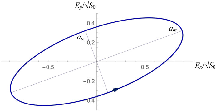
FIGURE 5. Polarization ellipse of the object wave (10) reflected from the back surface of the sample, calculated according to the numerical data of Eqs. (2)–(4), (6), (20).

Another possible way involves the Stokes parameters [34, 38, 39]. Based on the Jones vector (10), the Stokes parameters can be presented in the form

$\begin{array}{c}{S}_o={\left|E_{2x}\right|}^2+{\left|E_{2y}\right|}^2={\left[E_0{r}_2{\left(1-r_1\right)}^2\right]}^2,S_1={\left|E_{2x}\right|}^2-{\left|E_{2y}\right|}^2=S_o\left(1-2{\sin }^2\gamma {\sin }^{2}2\alpha \right),\hfill \\ S_2=2\mathrm{R}\mathrm{e}\left(E_{2y}{E}_{2x}^{*}\right)=2S_o{\sin }^2\gamma \sin 2\alpha \cos 2\alpha ,S_3=2\mathrm{I}\mathrm{m}\left(E_{2y}{E}_{2x}^{*}\right)=S_o\sin 2\gamma \sin 2\alpha \hfill \end{array}(26)$

and the known relation connecting the Stokes parameter $S_3$ with the major and minor polarization-ellipse semi-axes [38] $a_m$ and $a_n$ (see Figure 5) can be employed:

$a_{m,n}=\frac{1}{\sqrt{2}}{\left(S_o\pm \sqrt{S_0^2-S_3^2}\right)}^{1/2}$

whence, in view of (26),

$\sin 2\gamma \sin 2\alpha =\pm \frac{2a_m/a_n}{1+{\left(a_m/a_n\right)}^2}(27)$

and the positive (negative) sign corresponds to the counter-clockwise (clockwise) sense of the field-vector rotation, when seeing against the beam propagation (see Figure 5).

In particular, for the ellipse of Figure 5 that illustrates the situation of Eqs. 10, 11, $a_{2y}/a_{2x}=0.509$, and Eq. 25 means that $\sin \gamma \sin 2\alpha =0.453.$ In combination with Eq. 23 this gives

$\sin 2\alpha =0.6431,\alpha =20.01°;\sin \gamma =0.7044,\gamma =0.7816(28)$

in good correspondence with the model assumptions. Alternatively, the axes’ ratio measured for the modeled polarization ellipse presented in Figure 5 gives an additional equation in the form

$\sin 2\gamma \sin 2\alpha =0.6317$

which, again, supplies an independent channel for extracting $\alpha$ and $\gamma$ [and expectedly leads to practically the same results as (28)].

5 PS-OCT diagnostics of the sub-surface tissue variations

In some cases, near-surface nanosized layers of a lamella exist, in which the orientation of collagen fibers differs from the predominant orientation characteristic for deeper (volume) layers. In particular, this can appear as a result of the cornea damage [24]. Such a situation is illustrated by Figure 6 where the near-surface layer (NSL) with thickness d₁ is shown (in practice, the d₁ values of the order of 0.1 μm may occur [40]). The cornea pathology is often coupled with the waviness of its NSL: in this layer, the collagen fibers are no longer parallel to the nominal lamella plane (x, y) (see Figure 1) but experience wavelike deformations orthogonal to it [18, 23, 39]. Locally, within a single analyzed area of the size δx (see Section 2; Eq. 7), this looks as if the near-surface fibers, being parallel to each other, make a certain angle β with the “main” lamella plane (x, y); their in-plane orientation α remains unchanged. Then, with changing angle β, the birefringence (1) and the mean refractive index (2) are also changing, and the medium parameters vary over the sample depth. It appears that, despite the subwavelength sizes of such inhomogeneities, the sensitive PS-OCT techniques provides reliable means for their detection and quantitative characterization.

FIGURE 6

FIGURE 6. Formation of the reflected waves in presence of the near-surface nanolayer: (1a) front surface of the sample, (1b) boundary between the NSL and the sample volume, (2) back surface. Layers d₁ and d₂ form the total sample thickness, d₁ + d₂ = d.

The birefringence $∆n_a\left(\beta \right)$ and the mean refractive index ${\overline{n}}_a\left(\beta \right)$ of the NSL depend on the angle $\beta$ as [40, 41]

$∆n_a\left(\beta \right)=n_s\left(\beta \right)-n_o,{\overline{n}}_a\left(\beta \right)=\frac{n_o+n_s\left(\beta \right)}{2}(29)$

where

$n_s\left(\beta \right)=\frac{n_o{n}_e}{\sqrt{n_o^2{\cos }^2\beta +n_e^2{\sin }^2\beta }}.(30)$

Such a difference in the optical properties induces additional reflection at the boundary between the NSL and the main lamella volume. As a result, instead of the single front-surface reflection with the coefficient $r_1$ (12) considered in Section 3, one must analyze the situation with two consecutive reflection boundaries (Figure 6) characterized by the β-dependent Fresnel coefficients

$r_{1a}=\frac{\left|n_m-{\overline{n}}_a\left(\beta \right)\right|}{\left|n_m+{\overline{n}}_a\left(\beta \right)\right|},r_{1b}=\frac{\left|\overline{n}-{\overline{n}}_a\left(\beta \right)\right|}{\left|\overline{n}+{\overline{n}}_a\left(\beta \right)\right|}(31)$

where $n_m$ is the refractive index of the external medium (cf. Eq. 12) and $\overline{n}$ is the mean refractive index of the lamella volume (2). Note that according to Eq. 30, when $\beta \to 0$, $n_s\left(\beta \right)\to n_s\left(0\right)=n_e$, and the difference between the “near-surface” (29) and “volume” (2) optical parameters expectedly vanishes ($r_{1a}\to r_1$ (12), and $r_{1b}\to 0$).

Additionally, the phase retardation and polarization transformation in the NSL d₁ also differ from those of the lamella volume. These can be described by the Jones matrix M_a(α_a, β) which differs from the matrix (8) by replacements

${\gamma \to \gamma }_a\left(\beta \right)=k∆n_a\left(\beta \right)d_1,\alpha \to {\alpha }_a,$

(regarding that the angle ${\alpha }_a$ of the collagen fibers’ orientation in the NSL may deviate from its volume counterpart $\alpha$ presented in Eq. 8). Accordingly, the rest of the lamella (layer between planes 1b and 2, Figure 6) is described by the Jones matrix (8) where

${d\to d-d}_1=d_2,{\gamma \to \gamma }_b\left(d_2\right)=k∆n{d}_2.$

The calculations can be simplified due to the fact that for small values of $∆n=n_e-n_o$ [40],

$∆n_a\left(\beta \right)\approx \left(n_e-n_o\right){\cos }^2\beta ,{\gamma }_a\left(\beta \right)\approx k\left(n_e-n_o\right)d_1{\cos }^2\beta .$

Then, combining reflections from the boundaries 1a, 1b and 2 (Figure 6) and introducing the phase π-jumps where appropriate, one can easily find the complex amplitudes of the object-wave constituents, ${\mathbf{E}}_{Ob}={\mathbf{E}}_{1a}+{\mathbf{E}}_{1b}+{\mathbf{E}}_2$, generated by the incident probing wave ${\mathbf{E}}_0=E_0\left(\begin{array}{c}-1\\ 0\end{array}\right)$:

(i) wave reflected by the front surface 1a (Figure 6),

${\mathbf{E}}_{1a}=\left(\begin{array}{c}{E}_{1ax}\\ E_{1ay}\end{array}\right)=r_{1a}{e}^{i\pi }{E}_0=r_{1a}{E}_0\left(\begin{array}{c}1\\ 0\end{array}\right);(32)$

(ii) wave reflected by the inner interface 1b (Figure 6),

${\mathbf{E}}_{1b}=\left(\begin{array}{c}{E}_{1bx}\\ E_{1by}\end{array}\right)=E_0\left(\begin{array}{c}{\left(1-r_{1a}\right)}^2{r}_{1b}{e}^{2i{\delta }_a\left(\beta \right)}\left(\cos {\gamma }_a+i\sin {\gamma }_a\cos 2{\alpha }_a\right)\\ \left(1-r_{1a}\right)r_{1b}{e}^{2i{\delta }_a\left(\beta \right)}i\left(\sin {\gamma }_a\sin 2{\alpha }_a\right)\end{array}\right);(33)$

(iii) wave reflected by the back surface 2 (Figure 6),

${\mathbf{E}}_2=\left(\begin{array}{c}{E}_{2x}\\ E_{2y}\end{array}\right)=E_0\left(\begin{array}{c}-{\left(1-r_{1a}\right)}^2{\left(1-r_{1b}\right)}^2{r}_2{e}^{2i\left[{\delta }_a\left(\beta \right)+{\delta }_b\right]}{A}_{2x}\\ -\left(1-r_{1a}\right){\left(1-r_{1b}\right)}^2{r}_2{e}^{2i\left({\delta }_a\left(\beta \right)+{\delta }_b\right)+\pi /2}{A}_{2y}\end{array}\right).(34)$

In (Eqs. 32–34),

${\delta }_a\left(\beta \right)=k{\overline{n}}_a\left(\beta \right)d_1,{\delta }_b=k\overline{n}{d}_2(35)$

and

$A_{2x}=\cos {\gamma }_a\cos {\gamma }_b-\cos 2\left(\alpha -{\alpha }_a\right)\sin {\gamma }_a\sin {\gamma }_b+\frac{1}{2}i\left\{\cos {\gamma }_a\cos {\gamma }_b\left[\cos 2\alpha +\cos 2\left(\alpha -{2\alpha }_a\right)\right]-2\sin 2\left(\alpha -{\alpha }_a\right)\sin 2{\alpha }_a\sin {\gamma }_a+2\cos 2{\alpha }_a\cos {\gamma }_b\sin {\gamma }_a\right\};(36)$

$A_{2y}=\sin {\gamma }_b\left[{\cos }^2\frac{{\gamma }_a}{2}\sin 2\alpha +{\sin }^2\frac{{\gamma }_a}{2}\sin 2\left(\alpha -2{\alpha }_a\right)\right]+\cos {\gamma }_b\sin 2{\alpha }_a\sin {\gamma }_a.(37)$

The total field observed in the interferometer of Figure 2 is obtained by a superposition of the object waves (32)–(34) and the reference wave ${\mathbf{E}}_R$ taken in the form (13a) or (13b):

$\mathbf{E}={\mathbf{E}}_R+{\mathbf{E}}_{Ob}={\mathbf{E}}_R+{\mathbf{E}}_{1a}+{\mathbf{E}}_{1b}+{\mathbf{E}}_2.(38)$

Then, similarly to Eqs. (14), (16), (18), (19), interferograms observed in the x- and y-channels of the setup illustrated by Figure 2 can be calculated.

Generally, further operations are quite similar to those considered in Section 5. To avoid inessential complications, we now omit the cumbersome analytical expressions for the interference patterns I_x, I_y in the x- and y-channels [analogs of Eqs. (18); (19)], and directly address the numerical simulations illustrated in Figures 7, 8. The calculations are performed for the same probing and reference waves as were accepted in Figures 3, 4; the lamella volume is characterized by the optical parameters (2), (3) and (20), that is, $\alpha =20°,\beta =0$, but its thickness is $d_2=1.9\mu \mathrm{m}$. The width of the NSL is accepted to equal $d_1=0.1$ μm (see Figure 6), and the NSL anisotropy is characterized by

${\alpha }_a=20°,\beta =30°.(39)$

FIGURE 7

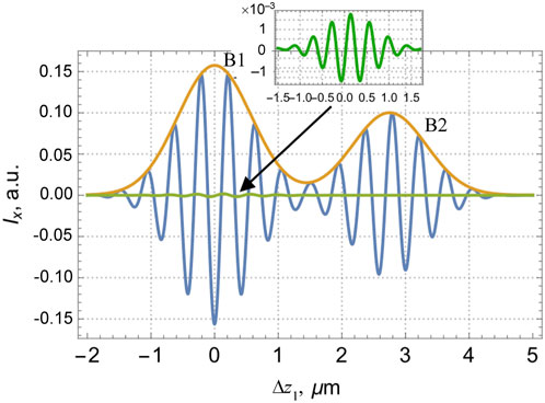
FIGURE 7. Variable component of the interferogram in the x-channel of the interferometer described by Figure 2 as a function of the reference–object waves’ path difference Δz₁ (15) for the lamella with NSL characterized by parameters (39). Green line shows the oscillations associated with the term $E_{1bx}$ (33) (supposed that all other object-wave contributions are suppressed).

FIGURE 8

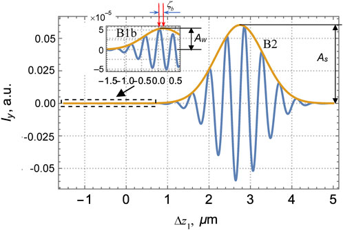
FIGURE 8. Variable component of the interferogram in the y-channel of the interferometer described by Figure 2 as a function of the reference–object waves’ path difference Δz₁ (15) for the lamella with NSL characterized by parameters (39).

It should be noted that the arguments of the coherence function (17) in the analogs of the interference contributions of (18), (19) will now include additional terms reflecting the specific phase retardations in the sub-layers d₁ and d₂ (see Figure 6): according to (33) and (34), instead of Eq. 15 one should take the coherence function arguments in the forms

$\Delta z_1\to \Delta z_1-\frac{{\delta }_a\left(\beta \right)}{k},\Delta z_2\to \Delta z_1-\frac{{\delta }_a\left(\beta \right)}{k}-\frac{{\delta }_b}{k}.(40)$

Here the first definition concerns the interference between ${\mathbf{E}}_R$ and ${\mathbf{E}}_{1b}$, and the second one relates to the terms describing the interference between ${\mathbf{E}}_R$ and ${\mathbf{E}}_2$, whereas ${\delta }_a\left(\beta \right)$ and ${\delta }_b$ are determined by Eq. 35. As a result, the interference patterns obtained for the lamella with a NSL look almost identical to their prototypes obtained for the homogeneous lamella (the only visible difference between Figure 7 and Figure 3, Figure 8 and Figure 4 is that the DC component is subtracted in Figures 7, 8).

Nevertheless, small distinctions due to the NSL do exist. For example, in the x-channel (Figure 7), the interference signal originating from the reflection at the boundary 1b (Figure 6) is two orders of magnitude lower than the signal originating from the front surface 1a, and the oscillations of both signals overlap inside the interference band B1, so they cannot be distinguished visually. To visualize the NSL-induced effects, in Figure 7 the green curve shows the “pure” NSL-attributed signal component observable under hypothetic conditions where all other components are suppressed. However, despite its low absolute value with respect to the “main” B1 signal, this NSL contribution can be revealed via detailed analysis of the interference curves.

This fact looks more favorable in the y-channel where basically (i.e., in case of a homogeneous lamella where the NSL is absent) the contribution of the front-surface reflection B1 vanishes, and only the back-surface-induced interference band B2 is present (see Figure 4). Due to the NSL, the weak signal associated with the reflection at the inner boundary 1b appears, and, in contrast to the x-channel (Figure 7), it is not masked by the front-surface reflection whose contribution vanishes in the y-channel. A “weak” band B1b (see the inset in Figure 8) emerges in addition to the “strong” band B2 well seen in both Figures 4, 8. Despite the weakness, the signal of B1b can be filtered and registered with a proper accuracy.

Then, operating as in Section 3 when determining the B2 maximum position, one can find the position of the B1b maximum (denoted as ζ_b in Figure 8), which corresponds to zero retardation (40), i.e.,

${\zeta }_b={\delta }_a\left(\beta \right)/k,{\overline{n}}_a\left(\beta \right)d_1={\zeta }_b(41)$

where the first Eq. 35 has been employed. This result gives a key to determining the NSL thickness d₁. In particular, according to Figure 8, ζ_b = 0.137 μm, and, neglecting the small difference between ${\overline{n}}_a\left(\beta \right)$ and $\overline{n}$ of Eq. 2, one obtains d₁ = 99.6 nm in agreement with the value accepted upon modeling. Note that the B2 maximum in Figures 7, 8 practically preserves its position observed for the homogeneous lamella (Figures 3, 4) that corresponds to $\Delta z_1=2.75$ μm but now, according to (40), this means

${\delta }_a\left(\beta \right)/k+{\delta }_b/k={\zeta }_b+\overline{n}{d}_2=2.75\mu m(42)$

and $d_2=1.901$ μm in agreement with the initial data.

Therefore, the presence of the band B1b and position of its “weak” envelope enables the NSL identification and, in the first approximation, measurement of its absolute thickness. Remarkably, even a subwavelength thickness can be reliably quantified with a rather large coherence length accepted (see Eq. 6). However, the important data on the NSL anisotropy, especially, its optical axis orientation (see Eq. 39) are not available from the above-described measurements.

Additional information can be extracted from the amplitudes of the object waves. In principle, the NSL optical properties can be determined if either of the reflection coefficients (31) is known, which, in turn, can be found from the reflected wave intensity. Yet, direct measurements of the reflection coefficients are hardly reliable because of many non-controllable factors associated with the wave transformations in various elements of the optical arrangement of Figure 2 and affecting the object wave amplitude. To avoid this ambiguity, comparative measurements of amplitudes of different elements of the same interferogram may be helpful. For example, the radiation belonging to the “weak” B1b and “strong” B2 bands of the interferogram in Figure 8 pass the same optical elements and experience the same non-controllable distortions but the ratio of their amplitudes, “weak” A_w and “strong” A_s, is free of these distortions and only depends on the sample characteristics. Moreover, with the use of Eqs. (32) – (38), the same procedures that lead to the interference curves of Figures 7, 8 enable to obtain the relation between A_w/A_s and the NSL anisotropy in the graphic form (Figure 9).

FIGURE 9

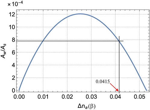
FIGURE 9. Ratio of the “weak” A_w and “strong” A_s amplitudes (see Figure 8) as a function of the NSL anisotropy $∆n_a\left(\beta \right)$ (29), calculated for the parameters (2)–(4), (6) and (20). The thin horizontal line corresponds to the value A_w/A_s = 7.85⋅10⁻⁴ obtained from Figure 8, thin vertical line indicates the resultant value of $∆n_a\left(\beta \right)=0.0415$.

Figure 9 is calculated for the same input data as Figures 7, 8, except that $0<\beta <90°$ and $0<{∆n}_a\left(\beta \right)<∆n$ are variable. The weak amplitude A_w expectedly vanishes on both edges of this interval because at $\beta =0$, ${∆n}_a\left(0\right)=∆n$, the difference between the NSL and the volume vanishes (lamella is homogeneous), while at $\beta =90°$, ${∆n}_a\left(0\right)=0$, the NSL anisotropy vanishes, and the y-component of the wave reflected from the inner boundary 1b does not exist.

Thus, the graphs of Figure 8 yield A_s = 0.065, A_w = 5.1⋅10⁻⁵, and A_w/A_s = 7.85⋅10⁻⁴. In Figure 9, two values of ${∆n}_a\left(\beta \right)$ satisfy this condition; we choose ${∆n}_a\left(\beta \right)=0.0415$ which is closer to the volume value (2). Accordingly, $n_s\left(\beta \right)=n_o+{∆n}_a\left(\beta \right)=1.390$ and ${\overline{n}}_a\left(\beta \right)=1.369$ (see Eqs. (29); (30)). These data practically solve the problem of the NSL optical properties characterization, and they well correspond with the values ${∆n}_a\left(\beta \right)=0.0392$ and $\overline{n}\left(\beta \right)=1.3681$ initially accepted for calculations. Further, using Eqs. (29) and (30), the data on the NSL optical-axis orientation can be extracted: $\beta =26.5°$, which also shows a reasonable agreement with the previously accepted value (39).

This simple example shows that the PS-OCT technique enables a rather complete and accurate characterization even of such weak and subwavelength-size inhomogeneities as the NSL. Obviously, the similar procedures can be used for the detection and characterization of additional internal boundaries, if these exist, thus providing a detailed non-invasive diagnostics of the sample fine structure.

6 Conclusion

In this paper, we present some results of the modeling of the PS-OCT procedure for diagnostics of optically anisotropic biological tissues. The information is recovered via interference with the controllable reference wave in a modified Mach–Zehnder interferometer with two output channels responsible for the two orthogonal polarization states. The amplitude of the interference signal and its dependence on the reference wave phase retardation allow to extract the data on the sample longitudinal inhomogeneity. The longitudinal resolution of the method depends on the coherence length $l_c$ but in favorable conditions can be less than $\sim 0.1l_c$. The lateral resolution depends on the probing-radiation focal spot and is determined by the numerical aperture of the objective and by the central wavelength ${\lambda }_0$. Upon reasonable requirements to the focus depth permitting the longitudinal scanning of samples with a few-micrometer thickness, the lateral resolution $\delta x\sim 2{\lambda }_0\sim 1.8\mu \mathrm{m}$ is possible. Such parameters noticeably exceed the accuracy available with other non-invasive approaches to the structure reconstruction, e.g., of the lamellae forming the eye cornea [40, 41]. Besides, our approach can be realized in the fully automatic regime, under the CPU control, which additionally contributes to the diagnostics accuracy and makes the procedure less time-consuming.

As immediate results, the interference measurements enable to determine the depths where the sample optical properties abruptly change (positions of the external and internal boundaries) and the parameters of separate layers between the boundaries (their widths and the values of ordinary $n_o$ and extraordinary $n_e$ refractive indices). The measuring approach discussed in the paper is naturally combined with the ellipsometric characterization of the object waves, which gives additional information on the sample’s optical anisotropy. Following to the known concepts of the lamellae’s structure [25–30], these data permit to learn the local alignment of the collagen fibers: (i) angle $\beta$ between the plane to which the fibers are (locally) parallel and the main lamella plane, which is supposed to coincide with the coordinate plane (x, y), and (ii) angle $\alpha$ of the fibers’ orientation with respect to the reference axis x within the (x, y) plane.

An important advantage of the proposed approach is that it permits to detect and quantitatively characterize a thin near-surface lamella layer with a non-zero $\beta$, even if its thickness is ∼100 nm and the mean refractive index ${\overline{n}}_a\left(\beta \right)$ differs from the index $\overline{n}$ of a non-perturbed lamella less than by 1% (Section 5). Remarkably, such impressive results are available in a contactless way, free of accompanying damage to the lamella surface [16, 17].

For simplicity, and in agreement with the common laboratory conditions, the simulations were performed for isolated lamella samples situated within the air environment. However, the similar results can be obtained for the lamella samples in the natural biological environment; the only difference is that in Eq. 12, instead of $n_m=1$, the refractive index of the base medium $n_m=1.356$ [18] should be taken. Accordingly, the reflection coefficients of the main boundaries would be much smaller, $r_1=r_2=0.007$ (cf. Eq. 20). As a result, the magnitudes of reflected signals will decrease proportionally but these signals are still available for modern detectors, together with the whole information contained in their polarization and phase. In this situation, the relative “weight” of the internal reflection caused by the NSL boundary 1b (see Section 5; Figure 6) would increase essentially, which may be favorable for the NSL diagnostics.

At the same time, it should be emphasized that in this paper, only the first and the most evident applications of the proposed approach are described. Its further development will bring new useful improvements, which promise the enhanced accuracy and spatial resolution of the PS-OCT techniques. In particular, the principles of the sensitive detection and measurement of the “weak” interference signal originating from the NSL-boundary reflection (see the band B1b in Figure 8) can be elaborated in order to reveal not only the difference between the mean refractive indices ${\overline{n}}_a\left(\beta \right)$ and $\overline{n}$ but also the “residual” difference between the NSL and lamella main volume, which occurs when the mean indices coincide, $\overline{n}={\overline{n}}_a\left(\beta \right)$ (all the collagen fibers lies in mutually parallel planes but the optical axes’ orientations α_a in the NSL and α in the volume differ). Obviously, the methods described in the paper can be adapted to other optically anisotropic biological samples, and their applications will be useful for the solution of many specific diagnostic problems.

Data availability statement

The original contributions presented in the study are included in the article/Supplementary Material, further inquiries can be directed to the corresponding author.

Author contributions

OA: Conceptualization, Data curation, Project administration, Writing–original draft, Supervision. AB: Formal Analysis, Writing–review and editing, Conceptualization, Validation. CZ: Conceptualization, Data curation, Validation, Visualization, Writing–original draft. DI: Writing–original draft, Investigation, Software, Visualization. JZ: Conceptualization, Funding acquisition, Methodology, Project administration, Writing–review and editing. MC: Investigation, Methodology, Validation, Writing–original draft.

Funding

The author(s) declare financial support was received for the research, authorship, and/or publication of this article. Research Institute of Zhejiang University–Taizhou, Center for Modern Optical Technology, China; Ministry of Education and Science of Ukraine (project 610/22, #0122U001830).

Acknowledgments

The authors are grateful to S. G. Hanson (DTU Fotonik, Roskilde, Denmark) for fruitful discussion and ideas on the high-sensitive contactless PS-OCT diagnostics of the bio-tissue near-surface layers.

Conflict of interest

The authors declare that the research was conducted in the absence of any commercial or financial relationships that could be construed as a potential conflict of interest.

Publisher’s note

All claims expressed in this article are solely those of the authors and do not necessarily represent those of their affiliated organizations, or those of the publisher, the editors and the reviewers. Any product that may be evaluated in this article, or claim that may be made by its manufacturer, is not guaranteed or endorsed by the publisher.

Footnotes

¹Here and in the following text we frequently demonstrate the process of recovering the sample characteristics from the graphical information which, in turn, was calculated based on the preliminary assigned parameters. At first glance, these manipulations may seem senseless: obviously, starting from a certain set of parameters, we finally cannot arrive at something other than the same set of parameters. However, the calculation errors and inevitable graphical inaccuracies model, to a certain degree, the noise and measurement errors occurring in real systems, and the quality of reconstruction of the initial sample parameters in our examples meaningfully illustrates the efficiency of corresponding algorithms in real experimental situations.

References

1. Fujimoto JG. Optical and acoustical imaging of biological media. Comptes Rendus de l'Académie des Sci (2001) 2:1099–11.

CrossRef Full Text | Google Scholar

2. Huang D, Swanson EA, Lin CP, Schuman JS, Stinson WG, Chang W, et al. Optical coherence tomography. Science (1991) 254:1178–81. doi:10.1126/science.1957169

PubMed Abstract | CrossRef Full Text | Google Scholar

3. de Freitas AZ, Amaral MM, Raele MP. Optical coherence tomography: development and applications. In: FG Duarte, editor. Laser pulse phenomena and applications. Rijeka, Croatia: IntechOpen (2010). p. 409–32. doi:10.5772/12899

CrossRef Full Text | Google Scholar

4. Aumann S, Donner S, Fischer J, Mǘller F. Optical coherence tomography (OCT): principle and technical realization. In: JF Bille, editor. High resolution imaging in microscopy and ophthalmology. Cham: Springer (2019). p. 59–85. doi:10.1007/978-3-030-16638-0_3

CrossRef Full Text | Google Scholar

5. Everett M, Magazzeni S, Schmoll T, Kempe M. Optical coherence tomography: from technology to applications in ophthalmology. Translational Biophotonics (2021) 3:e202000012. doi:10.1002/tbio.202000012

CrossRef Full Text | Google Scholar

6. Pircher M, Hitzenberger CK, Schmidt-Erfurth U. Polarization sensitive optical coherence tomography in the human eye. Prog Retin Eye Res (2011) 30(6):431–51. doi:10.1016/j.preteyeres.2011.06.003

PubMed Abstract | CrossRef Full Text | Google Scholar

7. Harper DJ, Augustin M, Lichtenegger A, Eugui P, Reyes C, Glösmann M, et al. White light polarization sensitive optical coherence tomography for sub-micron axial resolution and spectroscopic contrast in the murine retina. Biomed Opt Express (2018) 9:2115–29. doi:10.1364/BOE.9.002115

PubMed Abstract | CrossRef Full Text | Google Scholar

8. Pircher M, Goetzinger E, Leitgeb R, Hitzenberger CK. Transversal phase resolved polarization sensitive optical coherence tomography. Phys Med Biol (2004) 49(7):1257. doi:10.1088/0031-9155/49/7/013

PubMed Abstract | CrossRef Full Text | Google Scholar

9. de Boer JF, Milner TE. Review of polarization-sensitive optical coherence tomography and Stokes vector determination. J Biomed Opt (2002) 7(3):359–71. doi:10.1117/1.1483879

PubMed Abstract | CrossRef Full Text | Google Scholar

10. Drexler W, Chen Y, Aguirre AD, Považay B, Unterhuber A, Fujimoto JG. Ultrahigh resolution optical coherence tomography. In: W Drexler, and J Fujimoto, editors. Optical coherence tomography. Cham: Springer (2015). p. 277–318. doi:10.1007/978-3-319-06419-2_10

CrossRef Full Text | Google Scholar

11. Torzicky T. Polarization sensitive optical coherence tomography at 1060 nm for retinal imaging. Austria: Medical University of Vienna (2014). Doctoral Thesis.

Google Scholar

12. Hee MR, Huang D, Swanson EA, Fujimoto JG. Polarization-sensitive low-coherence reflectometer for birefringence characterization and ranging. J Opt Soc Am B (1992) 9:903–8. doi:10.1364/JOSAB.9.000903

CrossRef Full Text | Google Scholar

13. Gotzinger E, Pircher M, Hitzenberger CK. High speed spectral domain polarization sensitive optical coherence tomography of the human retina. Opt Express (2005) 13:10217–29. doi:10.1364/OPEX.13.010217

PubMed Abstract | CrossRef Full Text | Google Scholar

14. Baumann B. Polarization-sensitive optical coherence tomography: a review of technology and applications. Appl Sci (2017) 7:474. doi:10.3390/app7050474

CrossRef Full Text | Google Scholar

15. de Boer JF, Hitzenberger CK, Yasuno Y. Polarization sensitive optical coherence tomography – A review [invited]. Biomed Opt Express (2017) 8:1838–73. doi:10.1364/BOE.8.001838

PubMed Abstract | CrossRef Full Text | Google Scholar

16. Pierce MC, Shishkov M, Park BH, Nassif NA, Bouma BE, Tearney GJ, et al. Effects of sample arm motion in endoscopic polarization-sensitive optical coherence tomography. Opt Express (2005) 13:5739–49. doi:10.1364/OPEX.13.005739

PubMed Abstract | CrossRef Full Text | Google Scholar

17. Van der Sijde JN, Karanasos A, Villiger M, Bouma BE, Regar E. First-in-man assessment of plaque rupture by polarization-sensitive optical frequency domain imaging in vivo. Eur Heart J (2016) 37:1932. doi:10.1093/eurheartj/ehw179

PubMed Abstract | CrossRef Full Text | Google Scholar

18. Bron AJ. The architecture of the corneal stroma. Br J Ophthalmol (2001) 85:379–83. doi:10.1136/bjo.85.4.379

PubMed Abstract | CrossRef Full Text | Google Scholar

19. Tuchin VV. Tissue Optics: Light scattering methods and instruments for medical diagnosis. 3rd ed. Bellingham, Washington: SPIE (2015). p. 988. doi:10.1117/3.1003040

CrossRef Full Text | Google Scholar

20. Meek KM, Knupp C. Corneal structure and transparency. Prog Retin Eye Res (2015) 49:1–16. doi:10.1016/j.preteyeres.2015.07.001

PubMed Abstract | CrossRef Full Text | Google Scholar

21. McCally RL, Farrell RA. Light scattering from cornea and corneal transparency. In: BR Masters, editor. Noninvasive diagnostic techniques in ophthalmology. New York, NY: Springer (1990). doi:10.1007/978-1-4613-8896-8_12

CrossRef Full Text | Google Scholar

22. Farrell RA, Freund DE, McCally RL. Research on corneal structure. Johns Hopkins APL Tech Dig (Applied Phys Laboratory) (1990) 11(1-2):191.

Google Scholar

23. Freegard T. The physical basis of transparency of the normal cornea. Eye (1997) 11:465–71. doi:10.1038/eye.1997.127

PubMed Abstract | CrossRef Full Text | Google Scholar

24. Gallagher B, Maurice D. Striations of light scattering in the corneal stroma. J Ultrastruct Res (1977) 61(1):100–14. doi:10.1016/s0022-5320(77)90009-0

PubMed Abstract | CrossRef Full Text | Google Scholar

25. Donohue DJ, Stoyanov BJ, McCally RL, Farrell RA. Numerical modeling of the cornea’s lamellar structure and birefringence properties. J Opt Soc Am A (1995) 12(7):1425–38. doi:10.1364/josaa.12.001425

PubMed Abstract | CrossRef Full Text | Google Scholar

26. Newton RH, Brown JY, Meek KM. Polarized light microscopy technique for quantitatively mapping collagen fibril orientation in cornea. Proc SPIE (1996) 2926. doi:10.1117/12.260805

CrossRef Full Text | Google Scholar

27. Winkler M, Shoa G, Xie Y, Petsche SJ, Pinsky PM, Juhasz T, et al. Three-dimensional distribution of transverse collagen fibers in the anterior human corneal stroma. Invest Ophthalmol Vis Sci (2013) 54(12):7293–301. doi:10.1167/iovs.13-13150

PubMed Abstract | CrossRef Full Text | Google Scholar

28. Abahussin M, Hayes S, Cartwright NEK, Kamma-Lorger CS, Khan Y, Marshall J, et al. 3D collagen orientation study of the human cornea using X-ray diffraction and femtosecond laser technology. Invest Ophthalmol Vis Sci (2009) 50(11):5159–64. doi:10.1167/iovs.09-3669

PubMed Abstract | CrossRef Full Text | Google Scholar

29. Boote C, Hayes S, Abahussin M, Meek KM. Mapping collagen organization in the human cornea: Left and right eyes are structurally distinct. Invest Ophthalmol Vis Sci (2006) 47(3):901–8. doi:10.1167/iovs.05-0893

PubMed Abstract | CrossRef Full Text | Google Scholar

30. Abass A, Hayes S, White N, Sorensen T, Meek KM. Transverse depth-dependent changes in corneal collagen lamellar orientation and distribution. J R Soc Interf (2015) 12:20140717. doi:10.1098/rsif.2014.0717

PubMed Abstract | CrossRef Full Text | Google Scholar

31.In: JF Bille, editor. High resolution imaging in microscopy and ophthalmology. New Frontiers in biomedical Optics. Heidelberg, Germany: Heidelberg University (2019). p. 407. doi:10.1007/978-3-030-16638-0

CrossRef Full Text | Google Scholar

32. Fercher AF, Drexler W, Hitzenberger CK, Lasser T. Optical coherence tomography – principles and applications. Rep Prog Phys (2003) 66(2):239. doi:10.1088/0034-4885/66/2/20

CrossRef Full Text | Google Scholar

33. Atchison DA, Smith G. Chromatic dispersions of the ocular media of human eyes. J Opt Soc Am A (2005) 22(1):29–37. doi:10.1364/josaa.22.000029

PubMed Abstract | CrossRef Full Text | Google Scholar

34. Born M, Wolf E. Principles of Optics. 7th ed. Cambridge: Cambridge University Press (1999). p. 952.

Google Scholar

35. Angelsky OV, Hanson SG, Zenkova CY, Gorsky MP, Gorodyns’ka NV. On polarization metrology (estimation) of the degree of coherence of optical waves. Opt Express (2009) 17:15623–34. doi:10.1364/OE.17.015623

PubMed Abstract | CrossRef Full Text | Google Scholar

36. Angelsky OV, Zenkova CY, Gorsky MP, Gorodyns’ka NV. On the feasibility for estimating the degree of coherence of waves at near field. Appl Opt (2009) 48:2784–8. doi:10.1364/AO.48.002784

PubMed Abstract | CrossRef Full Text | Google Scholar

37. Zenkova CY, Gorsky MP, Gorodyns’ka NV. The electromagnetic degree of coherence in the near field. J Optoelectronics Adv Mater (2010) 12:74–8.

Google Scholar

38. Angelsky OV, Mokhun II, Bekshaev AY, Zenkova CY, Zheng J. Polarization singularities: topological and dynamical aspects. Front Phys (2023) 11:1147788. doi:10.3389/fphy.2023.1147788

CrossRef Full Text | Google Scholar

39. Angelsky O, Bekshaev A, Hanson SG, Zenkova CY, Mokhun I, Zheng J. Structured light: ideas and concepts. Front Phys (2020) 8:114. doi:10.3389/fphy.2020.00114

CrossRef Full Text | Google Scholar

40. Yang B, Jan NJ, Brazile B, Voorhees A, Lathrop KL, Sigal IA. Polarized light microscopy for 3-dimensional mapping of collagen fiber architecture in ocular tissues. J Biophotonics (2018) 11(8):e201700356. doi:10.1002/jbio.201700356

PubMed Abstract | CrossRef Full Text | Google Scholar

41. Spiesz EM, Kaminsky W, Zysset PK. A quantitative collagen fibers orientation assessment using birefringence measurements: Calibration and application to human osteons. J Struct Biol (2011) 176(3):302–6. doi:10.1016/J.JSB.2011.09.009

PubMed Abstract | CrossRef Full Text | Google Scholar