Fuzzy M-fractional integrodifferential models: theoretical existence and uniqueness results, and approximate solutions utilizing the Hilbert reproducing kernel algorithm

This article proposes a new approach to solving fuzzy M-fractional integrodifferential models under strongly generalized differentiability using an innovative formulation of the characterization principle. The study presents theoretical effects on the existence-uniqueness of fuzzy two M-solutions and, thus, showcases the solvability of the fuzzy Volterra models. Moreover, the study offers numerical solutions using the Hilbert reproducing kernel algorithm in a new fuzzy look, utilizing two fitting Hilbert spaces. The proposed models and algorithms are under scrutiny, with particular attention given to the analysis of the series solution, the assessment of convergence, and the evaluation of error. The debated Hilbert approach is shown to be effective in solving several fractional Volterra problems under uncertainty, and the numerical impacts manifest the accuracy and competence of the algorithm. Overall, our work contributes to the advancement of mathematical tools for solving complex fractional Volterra problems under uncertainty and shows potential to impact various fields of science and engineering, as depicted in the utilized figures, tables, and comparative analysis. The findings of the study are evaluated based on the analysis conducted, and a numerical algorithm is presented in the final section, along with several suggestions for future research directions.

1 Introduction

In recent years, fuzzy calculus and fuzzy integrodifferential models have gained significant attention due to their ability to model complex real-world problems that are inherently imprecise or uncertain [1–3]. Fuzzy calculus extends traditional calculus by incorporating the concept of fuzzy sets, which allows for the representation of uncertain or vague data in a mathematical framework. Fuzzy integrodifferential models combine the concepts of fuzzy sets and integrodifferential equations to model systems that involve both memory and uncertainty. In contrast, fractional calculus has emerged as a mighty mathematical tool for the formation of complex systems in various fields of science and engineering [4–6]. Recently, there has been a growing fascination with extending the concepts of fractional calculus to fuzzy environments, where the parameters of the system are not precisely defined but are instead represented by fuzzy numbers. This has led to the development of fuzzy fractional calculus, which has shown promising results in modeling and analyzing complex systems under uncertainty [7–9]. In this article, we will explore the concept of fuzzy fractional calculus and its application to FM-FIDMs. We will discuss the fundamental concepts of fuzzy calculus and fractional M-calculus, and then show how the two concepts can be combined to form a powerful tool for modeling and analyzing fuzzy systems represented by Volterra patterns. We will also present some examples of FM-FIDMs and their solutions utilizing HRKA, showcasing the productivity of our approach.

HRKA is a powerful mathematical tool that has found numerous products in assorted areas of stochastics and nonlinear phenomena [10–12]. The algorithm is based on the theory of Hilbert spaces, which provides a framework for the study of functions and their properties. HRKA is particularly useful for solving problems involving function approximation, interpolation, and regression, and has been used in applications such as machine learning, signal processing, and control theory [13–22]. One of the key characteristics of HRKA is its ability to represent functions in terms of inner products, which allows for efficient computation of function values and derivatives. This property is closely related to the concept of reproducing kernels, which are positive definite functions that satisfy certain properties. The construction of the reproducing kernel is an important aspect of HRKA and involves finding a function that satisfies the reproducing property and other properties that ensure its suitability for the problem at hand.

HRKA is a powerful mathematical framework used in applied mathematics, applied physics, machine learning, and other fields [10–12]. It offers several advantages over other approaches when it comes to solving NLDMs. Some of the distinguishing features of HRKA are as follows:

1. Nonlinear modeling: HRKA can capture nonlinear relationships between variables, making it a powerful tool for modeling NLDMs.

2. Flexibility: HRKA is very flexible and can be used to model a wide range of NLDMs, including those with complex constraint conditions.

3. High-dimensional feature space: HRKA maps data points into a high-dimensional feature space, where linear methods can be used to perform nonlinear tasks. This makes it possible to solve complex NLDMs using simple successive techniques.

4. Reproducing property: HRKA has a unique property called the reproducing property, which allows the evaluation of functions in the reproducing Hilbert space at any point in the input space. This means that it can be used to interpolate solutions to NLDMs and make predictions at any point in the input space.

5. Regularization: HRKA uses regularization to control the complexity of the model and prevent overfitting. This is performed by introducing a penalty term in the objective function that penalizes large coefficients in the model.

Indeed, when using HRKA to solve NLDMs, these advantages translate into several distinct benefits.

1. Accuracy: The flexibility of HRKA allows it to accurately model complex NLDMs, producing solutions with high accuracy.

2. Efficiency: The use of high-dimensional feature space and simple successive techniques can make HRKA more computationally efficient than other methods for solving NLDMs.

3. Interpolation: The reproducing property of HRKA allows it to interpolate solutions to NLDMs, making it possible to accurately predict values at any point in the input space.

4. Regularization: The use of regularization helps prevent overfitting, producing more reliable solutions to NLDMs.

Generally, HRKA offers several advantages over other approaches when it comes to solving NLDMs. Its ability to model nonlinear relationships, flexibility, use of high-dimensional feature space, reproducing property, and regularization all contribute to its accuracy, efficiency, and ability to interpolate solutions.

This article delves into two important mathematical concepts: the existence-uniqueness and characterization theorems, and the simulated HRKA. In the first part, we explore the theorem’s significance in proving the existence-uniqueness of fuzzy two M-solutions, and we will discuss how the characterization theorem helps us provide a framework for understanding the proof. In the second part, we delve into HRKA, which is a powerful tool for analyzing numerical approximations and their properties. Through this, we will explore our requirements for the following general model:

$\left\{\begin{array}{l}{\mathcal{R}}_M^{\left\{\mathfrak{v},\mathfrak{w}\right\}}ẞ\left(ͷ\right)=\mathcal{h}\left(ͷ,ẞ\left(ͷ\right)\right)+{\int }_0^{ͷ}\mathcal{k}\left(ͷ,x,ẞ\left(x\right)\right)dx,\\ ẞ\left(0\right)=Ɯ.\end{array}\right.(1)$

Here, $ͷ\in \wp :=\left[\mathrm{0,1}\right]$, $x\in \left[0,ͷ\right]$, $\left.\mathfrak{v}\in \mathbb{D}≔(\mathrm{0,1}\right]$, $\mathfrak{w}>0$, $Ɯ\in {\mathbb{R}}_{\aleph }$, $ẞ\in \complement \left(\wp ,{\mathbb{R}}_{\aleph }\right)$, $\mathcal{h}\in \complement \left(\wp \times {\mathbb{R}}_{\aleph },{\mathbb{R}}_{\aleph }\right)$, and $\mathcal{k}\in \left({\wp }^2\times {\mathbb{R}}_{\aleph },{\mathbb{R}}_{\aleph }\right)$. Indeed, ${\mathcal{R}}_M^{\left\{\mathfrak{v},\mathfrak{w}\right\}}ẞ\left(ͷ\right)$ is the FM-D of order $\mathfrak{v},$ concerning the Mittag–Leffler parameter $\mathfrak{w}$, and ${\mathbb{R}}_{\aleph }$ denotes the set of fuzzy numbers.

FM-D is a relatively new concept in the field of fractional calculus. It was introduced as an innovative class of fractional derivatives that has some advantages over other fractional approaches, such as Riemann or Caputo derivatives. One of the main advantages of FM-D is that it preserves the chain rule of differentiation. This means that if we apply FM-D to a composite function, we can use the chain rule to simplify the result. This property is not shared by other fractional derivatives, which can make it difficult to apply them in practice. Another advantage of FM-D is that it is more closely related to the ordinary derivative than other fractional derivatives. In particular, it satisfies a version of the Leibniz rule, which allows us to differentiate products of functions naturally. This makes it easier to use FM-D in applications where we need to differentiate products of functions, such as in physics and engineering [23–28]. It also has some interesting mathematical properties that make it an attractive tool for studying fractional models. For example, it has been shown that FM-D can be used to obtain exact solutions for certain types of fractional models. This could be useful in applications where we need to solve NLDMs that involve fractional derivatives. Other theoretical and application results concerning fractional calculus patterns with several constraints and types can be collected from [29–35]. Overall, FM-D is a promising new tool in the branch of calculus, and it shows potential to be useful in a wide range of applications.

After the preliminary stage and the problem formulation phase, the study is structured as follows: Section 2 provides an overview of fuzzy calculus and FM-D. Section 3 introduces fuzzy FM-D as differentiation and continuity, followed by fuzzy FM-I as integration and inversion. In Section 4, we examine FM-FIDM as structures, tools, and steps, while Section 5 presents a new characterization theorem. Section 6 introduces HRKA in terms of structures and tools, and Section 7 implements HRKA as structures and tools. Section 8 showcases the numerical implementations and computed results. Finally, Section 9 presents the key points and summary of the study.

2 Outline of fuzzy calculus and FM-D

Herein, we will delve into the concept of fuzzy numbers, which are an essential tool in the fuzzy set theory. Fuzzy numbers are a generalization of traditional real numbers, allowing for uncertainty and imprecision to be incorporated into numerical values. We will explore the $\theta$-cut concerning fuzzy numbers, their metric structure, and their fundamental theorem, which establishes the relationship between fuzzy numbers and intervals. Additionally, we will discuss the concept of $\mathcal{H}$-difference.

Specifically, substitute $\mathbb{I}≔\left[\mathrm{0,1}\right]$ and $\forall \theta \in \mathbb{I}-\left\{0\right\}$, and set ${\left[Ɯ\right]}^{\theta }=\left\{ƻ\in \mathbb{R}\mathbb{|}Ɯ\left(ƻ\right)\ge \theta \right\}$ and ${\left[Ɯ\right]}^0=\overline{\left\{ƻ\in \mathbb{R}\mathbb{|}Ɯ\left(ƻ\right)>0\right\}}$. Then, $Ɯ\in {\mathbb{R}}_{\aleph }$ if ${\left[Ɯ\right]}^{\theta }$ is a compact convex in $\mathbb{R}$ and ${\left[Ɯ\right]}^1\ne \varphi$ [36]. So, if $Ɯ\in {\mathbb{R}}_{\aleph }$, then ${\left[Ɯ\right]}^{\theta }=\left[{Ɯ}_1\left(\theta \right),{Ɯ}_2\left(\theta \right)\right]$ whenever ${Ɯ}_1\left(\theta \right)=\min \left\{ƻ|ƻ\in {\left[Ɯ\right]}^{\theta }\right\}$ and ${Ɯ}_2\left(\theta \right)=\max \left\{ƻ|ƻ\in {\left[Ɯ\right]}^{\theta }\right\}$. Hitherto, ${\left[Ɯ\right]}^{\theta }$ is the $\theta$-cut of $Ɯ$. For simplicity, ${Ɯ}_{1\left(\theta \right)}≔{Ɯ}_1\left(\theta \right)$ and ${Ɯ}_{2\left(\theta \right)}≔{Ɯ}_2\left(\theta \right)$.

Theorem 1. [36] Presume that ${Ɯ}_{\mathrm{1,2}}:\mathbb{I}\to \mathbb{R}$ fulfills the following criterion: ${Ɯ}_1$ nondecreasing bounded and ${Ɯ}_2$ nonincreasing bounded, ${\lim }_{\theta \to {\mathcal{y}}^{-}}{Ɯ}_{\mathrm{1,2}\left(\theta \right)}={Ɯ}_{\mathrm{1,2}\left(\mathcal{y}\right)}$ and ${\lim }_{\theta \to 0^{+}}{Ɯ}_{\mathrm{1,2}\left(\theta \right)}={Ɯ}_{\mathrm{1,2}\left(0\right)}$, and $\forall \mathcal{y}\in \mathbb{I}-\left\{0\right\}$: ${Ɯ}_{1\left(1\right)}\le {Ɯ}_{2\left(1\right)}$. Then, $Ɯ:\mathbb{R}\to \mathbb{I}$ with $Ɯ\left(ƻ\right)=\sup \left\{\theta |{Ɯ}_{1\left(\theta \right)}\le ƻ\le {Ɯ}_{2\left(\theta \right)}\right\}$ belongs to ${\mathbb{R}}_{\aleph }$ with parameterization $\left[{Ɯ}_{1\theta },{Ɯ}_{2\theta }\right]$. Likewise, if ${Ɯ}_{\mathrm{1,2}}:\mathbb{I}\to \mathbb{R}$ belongs to ${\mathbb{R}}_{\aleph }$ with parameterization $\left[{Ɯ}_{1\left(\theta \right)},{Ɯ}_{2\left(\theta \right)}\right]$, then ${Ɯ}_{\mathrm{1,2}}$ meets the previously mentioned requirements.

For a more in-depth explanation, let $Ɯ,\overline{Ɯ}\in {\mathbb{R}}_{\aleph }$. If $\exists Ɯ\in {\mathbb{R}}_{\aleph }$ with $\overline{Ɯ}+Ɯ=Ɯ$, then $Ɯ$ entitled the $\mathcal{H}$-difference of $\left(Ɯ,\overline{Ɯ}\right)$ is denoted by $Ɯ\ominus \overline{Ɯ}$, whereas $\ominus$ implies constantly to the $\mathcal{H}$-difference being mindful of $Ɯ\ominus \overline{Ɯ}\ne Ɯ+\left(-1\right)\overline{Ɯ}=Ɯ-\overline{Ɯ}$. Whenever the $\mathcal{H}$-difference $Ɯ\ominus \overline{Ɯ}$ exists, ${\left[Ɯ\ominus \overline{Ɯ}\right]}^{\theta }=\left[{Ɯ}_{1\left(\theta \right)}-{\overline{Ɯ}}_{1\left(\theta \right)},{Ɯ}_{2\left(\theta \right)}-{\overline{Ɯ}}_{2\left(\theta \right)}\right]$.

A metric $\left({\mathbb{R}}_{\aleph },d_{\infty }\right)$ is complete with $d_{\infty }:{\mathbb{R}}_{\aleph }^2\to {\mathbb{R}}^{+}\cup \left\{0\right\}$ and $d_{\infty }\left(Ɯ,\overline{Ɯ}\right)=\underset{\theta \in \mathbb{I}}{\sup }\max \left\{\left|{Ɯ}_{1\left(\theta \right)}-{\overline{Ɯ}}_{1\left(\theta \right)}\right|,\left|{Ɯ}_{2\left(\theta \right)}-{\overline{Ɯ}}_{2\left(\theta \right)}\right|\right\}$. $ẞ\in \complement \left(\wp \to {\mathbb{R}}_{\aleph }\right)$ at ${ͷ}^{*}\in \wp$ provided $\forall \epsilon >0$ and $\forall ͷ\in \wp$; $\exists \delta >0$ with $d_{\infty }\left(ẞ\left(ͷ\right),ẞ\left({ͷ}^{*}\right)\right)<\epsilon$ whenever $\left|ͷ-{ͷ}^{*}\right|<\delta$. Undoubtedly, $ẞ$ is continuous over $\wp ;$ if it is continuous, $\forall ͷ\in \wp$. $\mathcal{h}\in \complement \left(\wp \times {\mathbb{R}}_{\aleph },{\mathbb{R}}_{\aleph }\right)$ at $\left({ͷ}^{*},z^{*}\right)$ in $\wp \times {\mathbb{R}}_{\aleph }$ provided $\forall \epsilon >0$ and $\exists \delta \left(\epsilon ,\theta \right)>0$ with $d_{\infty }\left(f\left(ͷ,z\right),f\left({ͷ}^{*},z^{*}\right)\right)<\epsilon$ whenever $\left|{ͷ}^{*}-ͷ\right|<\delta$ and $d_{\infty }\left(z,z^{*}\right)<\delta$, $\forall ͷ\in \wp$ and $\forall z\in {\mathbb{R}}_{\aleph }$. Similarly, for $\mathcal{k}\in \complement \left({\wp }^2\times {\mathbb{R}}_{\aleph }\to {\mathbb{R}}_{\aleph }\right)$. Indeed, if $\complement \left(\wp ,{\mathbb{R}}_{\aleph }\right)$ be the set of all continuous $ẞ:\wp \to {\mathbb{R}}_{\aleph }$ mapping, then $d_1:\complement \left(\wp ,{\mathbb{R}}_{\aleph }\right)\times \complement \left(\wp ,{\mathbb{R}}_{\aleph }\right)\to {\mathbb{R}}^{+}\cup \left\{0\right\}$ with $d_1\left({ẞ}_1,{ẞ}_2\right)=\underset{ͷ\in \wp }{\sup }\left(d_{\infty }\left({ẞ}_1\left(ͷ\right),{ẞ}_2\left(ͷ\right)\right)e^{-Ỽͷ}\right)$, $\forall {ẞ}_1,{ẞ}_2\in \complement \left(\wp ,{\mathbb{R}}_{\aleph }\right)$, where $Ỽ\in \mathbb{R}$ is fixed. It is evidenced in [37] that $\left(\complement \left(\wp ,{\mathbb{R}}_{\aleph }\right),d_1\right)$ is a complete metric.

Using a pair of fuzzy functions and the $\theta$-cut approach, the Zadeh extension principle allows us to perform fuzzy arithmetic operations in a fuzzy setting.

Theorem 2. [37] If $\mathcal{U}\in C\left({\mathbb{R}}^2\to \mathbb{R}\right)$, then $ẞ\in C\left({\mathbb{R}}_{\aleph }^2\to {\mathbb{R}}_{\aleph }\right)$ and ${\left[ẞ\left(Ɯ,\overline{Ɯ}\right)\right]}^{\theta }=\mathcal{U}\left({\left[Ɯ\right]}^{\theta },{\left[\overline{Ɯ}\right]}^{\theta }\right)$, $\forall Ɯ,\overline{Ɯ}\in {\mathbb{R}}_{\aleph },$ and $\theta \in \mathbb{I}$.

In the following paragraphs, we will explore the concept of FM-D, which is a memorization of conformable scaling derivative. We will start by defining FM-D and discussing its mathematical properties, including its relationship to classical derivatives, and its applications in various fields of study. Additionally, we will examine several related results that shed light on the behavior of FM-D and its significance in understanding the complexity of real-world phenomena.

FM-D has several tools in engineering and applied sciences [23–28]. For example, it can be used to model non-Newtonian fluids, which exhibit complex and nonlinear behaviors that cannot be described by ordinary derivatives. In addition, it can be used to simulate fractional-order systems, like electrical circuits and control systems, which exhibit memory effects and other non-ideal behaviors. However, FM-D is a generalization of the classical derivative to noninteger values of the differentiation of order $\mathfrak{v}\in \mathbb{D}$ concerning the Leffler parameter $\mathfrak{w}$.

Definition 1. [23] Let $\mathcal{U}\in C\left(\wp \to \mathbb{R}\right)$. Then, FM-D of order $\mathfrak{v}\in \mathbb{D}$ concerning the Leffler parameter $\mathfrak{w}$ of $\mathcal{U}$ at $ͷ\in \wp$ is

${\mathcal{R}}_M^{\left\{\mathfrak{v},\mathfrak{w}\right\}}\mathcal{U}\left(ͷ\right)=\left\{\begin{array}{l}\underset{\epsilon \to 0}{\lim }\frac{\mathcal{U}\left(ͷ{\mathbb{E}}_{\mathfrak{w}}\left(\epsilon {ͷ}^{-\mathfrak{v}}\right)\right)-\mathcal{U}\left(ͷ\right)}{\epsilon },ͷ>0,\\ \underset{ͷ\to 0^{+}}{\lim }{\mathcal{R}}_M^{\mathfrak{v},\mathfrak{w}}\mathcal{U}\left(ͷ\right),ͷ=0.\end{array}\right.(2)$

Herein, ${\mathbb{E}}_{\mathfrak{w}}\left(ͷ\right)={\displaystyle \sum _{\mathcal{y}=0}^{\infty }}\frac{{ͷ}^{\mathcal{y}}}{{\mathrm{\Gamma }}_{\mathfrak{w}\mathcal{y}+1}}$ is the infinite Mittag–Leffler operator with $\mathfrak{w}>0$ and $ͷ>0$. It is assumed that $\mathcal{U}$ is $\left\{\mathfrak{v},\mathfrak{w}\right\}$-differentiable whenever $\mathcal{U}$ is differentiable $\forall ͷ\in \wp$. Indeed, ${\mathcal{R}}_M^{\left\{\mathfrak{v},\mathfrak{w}\right\}}\mathcal{U}\left(0\right)$ exists whenever $\underset{ͷ\to 0^{+}}{\lim }{\mathcal{R}}_M^{\left\{\mathfrak{v},\mathfrak{w}\right\}}\mathcal{U}\left(ͷ\right)$ exists.

Using the FM-D definition as our foundation, we can showcase the linearity of FM-D, as well as its adherence to fundamental rules, such as the product, composition, quotient, and chain rules for two $\left\{\mathfrak{v},\mathfrak{w}\right\}$-differentiable functions. Additionally, the derivative of a constant is indeed zero. However, whenever $\mathcal{U}\in \wp \to \mathbb{R}$ is $\left\{\mathfrak{v},\mathfrak{w}\right\}$-differentiable at ${ͷ}^{*}\in \wp$ with $\mathfrak{v}\in \mathbb{D}$ and $\mathfrak{w}>0$, then $\mathcal{U}$ is continuous at ${ͷ}^{*}$. Indeed, what sets FM-D apart from other fractional approaches is its primary and fundamental differentiation rule, which is ${\mathcal{R}}_M^{\left\{\mathfrak{v},\mathfrak{w}\right\}}\mathcal{U}\left(ͷ\right)=\frac{{ͷ}^{1-\mathfrak{v}}}{{\mathrm{\Gamma }}_{\mathfrak{w}+1}}{\mathcal{U}}^{\prime }\left(ͷ\right)$. For example, ${\mathcal{R}}_M^{\left\{\mathfrak{v},\mathfrak{w}\right\}}\left(\frac{{\mathrm{\Gamma }}_{\mathfrak{w}+1}}{\mathfrak{v}}{ͷ}^{\mathfrak{v}}\right)=1$ and ${\mathcal{R}}_M^{\left\{\mathfrak{v},\mathfrak{w}\right\}}\left(1\right)=0$.

Definition 2. [23] Let $\mathcal{U}\in C\left(\wp \to \mathbb{R}\right)$. Then, FM-I of order $\mathfrak{v}\in \mathbb{D}$ with $\mathfrak{w}>0$ of $\mathcal{U}$ at $ͷ\in \wp$ is

$I_M^{\left\{\mathfrak{v},\mathfrak{w}\right\}}\mathcal{U}\left(ͷ\right)={\mathrm{\Gamma }}_{\mathfrak{w}+1}{\int }_0^{ͷ}\frac{\mathcal{U}\left(x\right)}{x^{1-\mathfrak{v}}}dx.(3)$

Next, theoretical results are employed to elucidate the relationship between FM-D and FM-I behaviors. Specifically, the inversion formula and the fundamental theorem of calculus are utilized in the sense of fractional M-calculus.

Theorem 3. [23] For $\mathfrak{v}\in \mathbb{D}$, $\mathfrak{w}>0$, and $\forall ͷ\in \wp$, then

i. If $\mathcal{U}\in C\left(\wp \to \mathbb{R}\right)$ and $I_M^{\left\{\mathfrak{v},\mathfrak{w}\right\}}\mathcal{U}$ exists, then ${\mathcal{R}}_M^{\left\{\mathfrak{v},\mathfrak{w}\right\}}\left(I_M^{\left\{\mathfrak{v},\mathfrak{w}\right\}}\mathcal{U}\left(ͷ\right)\right)=\mathcal{U}\left(ͷ\right).$

ii. If $\mathcal{U}\in \wp \to \mathbb{R}$ is $\left\{\mathfrak{v},\mathfrak{w}\right\}$-differentiable and $I_M^{\left\{\mathfrak{v},\mathfrak{w}\right\}}\mathcal{U}$ exists, then $I_M^{\left\{\mathfrak{v},\mathfrak{w}\right\}}\left({\mathcal{R}}_M^{\left\{\mathfrak{v},\mathfrak{w}\right\}}\mathcal{U}\left(ͷ\right)\right)=\mathcal{U}\left(ͷ\right)-\mathcal{U}\left(0\right).$

For additional information on the FM-D, FM-I, and Mittag–Leffler parameter, including further results, historical notes, characteristics, applications, and methods, please refer to [23–28].

3 Fuzzy FM-D: differentiation and continuity

Foremost, we present the fuzzy FM-D concept, its definitions, and its properties. We utilize a new strongly generalized fuzzy FM-D delineation for a $ẞ$ value of order $\mathfrak{v}\in \mathbb{D}$ with $\mathfrak{w}>0$ in two inclusive phases. The derivative representation theory and continuity results are also exhibited.

Definition 3. Let $ẞ\in \complement \left(\wp ,{\mathbb{R}}_{\aleph }\right)$ with $\mathfrak{v}\in \mathbb{D}$ and $\mathfrak{w}>0$. Then, $ẞ$ is a strongly generalized fuzzy FM-D at $ͷ\in \wp$ if $\exists {\mathcal{R}}_M^{\left\{\mathfrak{v},\mathfrak{w}\right\}}ẞ\left(ͷ\right)\in {\mathbb{R}}_{\aleph }$ with one among the succeeding is met:

i. $\forall ϵ>0$ small-scale, $ẞ\left(ͷ{\mathbb{E}}_{\mathfrak{w}}\left(\epsilon {ͷ}^{-\mathfrak{v}}\right)\right)\ominus ẞ\left(ͷ\right)$ exists, and

${\mathcal{R}}_M^{\left\{\mathfrak{v},\mathfrak{w}\right\}}ẞ\left(ͷ\right)=\left\{\begin{array}{l}\underset{\epsilon \to 0}{\lim }\frac{ẞ\left(ͷ{\mathbb{E}}_{\mathfrak{w}}\left(\epsilon {ͷ}^{-\mathfrak{v}}\right)\right)\ominus \stackrel{\sim }{f}\left(ͷ\right)}{\epsilon },ͷ>0,\\ \underset{ͷ\to 0^{+}}{\lim }{\mathcal{R}}_M^{\left\{\mathfrak{v},\mathfrak{w}\right\}}ẞ\left(ͷ\right),ͷ=0.\end{array}\right.(4)$

ii. $\forall ϵ>0$ small-scale, $ẞ\left(ͷ\right)\ominus ẞ\left(ͷ{\mathbb{E}}_{\mathfrak{w}}\left(\epsilon {ͷ}^{-\mathfrak{v}}\right)\right)$ exists, and

${\mathcal{R}}_M^{\left\{\mathfrak{v},\mathfrak{w}\right\}}ẞ\left(ͷ\right)=\left\{\begin{array}{l}\underset{\epsilon \to 0}{\lim }\frac{ẞ\left(ͷ\right)\ominus ẞ\left(ͷ{\mathbb{E}}_{\mathfrak{w}}\left(\epsilon {ͷ}^{-\mathfrak{v}}\right)\right)}{-\epsilon },ͷ>0,\\ \underset{ͷ\to 0^{+}}{\lim }{\mathcal{R}}_M^{\left\{\mathfrak{v},\mathfrak{w}\right\}}ẞ\left(ͷ\right),ͷ=0.\end{array}\right.(5)$

Definition 4. Let $ẞ\in C\left(\wp ,{\mathbb{R}}_{\aleph }\right)$ with $\mathfrak{v}\in \mathbb{D}$ and $\mathfrak{w}>0$. Then,

i. $ẞ$ is apparently $\left\{\mathfrak{v}\left(1\right),\mathfrak{w}\right\}$-fuzzy FM-D on $\wp$ if $ẞ$ concerning (4) is $\left\{\mathfrak{v},\mathfrak{w}\right\}$-differentiable.

ii. $ẞ$ is apparently $\left\{\mathfrak{v}\left(2\right),\mathfrak{w}\right\}$-fuzzy FM-D on $\wp$ if $ẞ$ concerning (5) is $\left\{\mathfrak{v},\mathfrak{w}\right\}$-differentiable.

Undoubtedly, the fuzzy FM-Ds of $ẞ$ will be characterized as ${\mathcal{R}}_M^{\left\{\mathfrak{v}\left(1\right),\mathfrak{w}\right\}}ẞ$ and ${\mathcal{R}}_M^{\left\{\mathfrak{v}\left(2\right),\mathfrak{w}\right\}}ẞ$ in phases (i) and (ii), sequentially. The next termination pertains to the intersection of fuzzy FM-D and crisp differentiability.

Theorem 4. Let $ẞ\in \complement \left(\wp ,{\mathbb{R}}_{\aleph }\right)$ with $\mathfrak{v}\in \mathbb{D}$ and $\mathfrak{w}>0$. Then,

i. If $ẞ$ is $\left\{\mathfrak{v}\left(1\right),\mathfrak{w}\right\}$-fuzzy FM-D, then ${ẞ}_{1\left(\theta \right)}\left(ͷ\right)$ and ${ẞ}_{2\left(\theta \right)}\left(ͷ\right)$ are $\left\{\mathfrak{v},\mathfrak{w}\right\}$-differentiable on $\wp$ with

${\left[{\mathcal{R}}_M^{\left\{\mathfrak{v}\left(1\right),\mathfrak{w}\right\}}ẞ\left(ͷ\right)\right]}^{\theta }=\left[{\mathcal{R}}_M^{\left\{\mathfrak{v},\mathfrak{w}\right\}}{ẞ}_{1\left(\theta \right)}\left(ͷ\right),{\mathcal{R}}_M^{\left\{\mathfrak{v},\mathfrak{w}\right\}}{ẞ}_{2\left(\theta \right)}\left(ͷ\right)\right].(6)$

ii. If $ẞ$ is $\left\{\mathfrak{v}\left(2\right),\mathfrak{w}\right\}$-fuzzy FM-D, then ${ẞ}_{1\left(\theta \right)}\left(ͷ\right)$ and ${ẞ}_{2\left(\theta \right)}\left(ͷ\right)$ are $\left\{\mathfrak{v},\mathfrak{w}\right\}$-differentiable on $\wp$ with

${\left[{\mathcal{R}}_M^{\left\{\mathfrak{v}\left(2\right),\mathfrak{w}\right\}}ẞ\left(ͷ\right)\right]}^{\theta }=\left[{\mathcal{R}}_M^{\left\{\mathfrak{v},\mathfrak{w}\right\}}{ẞ}_{2\left(\theta \right)}\left(ͷ\right),{\mathcal{R}}_M^{\left\{\mathfrak{v},\mathfrak{w}\right\}}{ẞ}_{1\left(\theta \right)}\left(ͷ\right)\right].(7)$

Proof. Here, our attention will be directed toward (i), while a comparable proof can be utilized for (ii). Assuming that $ͷ\in \wp$ is fixed, according to the given assumptions, one obtains

${\left[ẞ\left(ͷ{\mathbb{E}}_{\mathfrak{w}}\left(\epsilon {ͷ}^{-\mathfrak{v}}\right)\right)\ominus ẞ\left(ͷ\right)\right]}^{\theta }=\left[{ẞ}_{1\left(\theta \right)}\left(ͷ{\mathbb{E}}_{\mathfrak{w}}\left(\epsilon {ͷ}^{-\mathfrak{v}}\right)\right)-{ẞ}_{1\left(\theta \right)}\left(ͷ\right),{ẞ}_{2\left(\theta \right)}\left(ͷ{\mathbb{E}}_{\mathfrak{w}}\left(\epsilon {ͷ}^{-\mathfrak{v}}\right)\right)-{ẞ}_{2\left(\theta \right)}\left(ͷ\right)\right].(8)$

Multiplying by $\frac{1}{\epsilon }$, we get

${\left[\frac{ẞ\left(ͷ{\mathbb{E}}_{\mathfrak{w}}\left(\epsilon {ͷ}^{-\mathfrak{v}}\right)\right)\ominus ẞ\left(ͷ\right)}{\epsilon }\right]}^{\theta }=\left[\frac{{ẞ}_{1\left(\theta \right)}\left(ͷ{\mathbb{E}}_{\mathfrak{w}}\left(\epsilon {ͷ}^{-\mathfrak{v}}\right)\right)-{ẞ}_{1\left(\theta \right)}\left(ͷ\right)}{\epsilon },\frac{{ẞ}_{2\left(\theta \right)}\left(ͷ{\mathbb{E}}_{\mathfrak{w}}\left(\epsilon {ͷ}^{-\mathfrak{v}}\right)\right)-{ẞ}_{2\left(\theta \right)}\left(ͷ\right)}{\epsilon }\right].(9)$

Passing to the limit, we get ${ẞ}_{1\left(\theta \right)}$ and ${ẞ}_{2\left(\theta \right)}$ as $\left\{\mathfrak{v},\mathfrak{w}\right\}$-differentiable on $\wp$ with

${\left[{\mathcal{R}}_M^{\left\{\mathfrak{v}\left(1\right),\mathfrak{w}\right\}}ẞ\left(ͷ\right)\right]}^{\theta }=\left[{\mathcal{R}}_M^{\left\{\mathfrak{v},\mathfrak{w}\right\}}{ẞ}_{1\left(\theta \right)}\left(ͷ\right),{\mathcal{R}}_M^{\left\{\mathfrak{v},\mathfrak{w}\right\}}{ẞ}_{2\left(\theta \right)}\left(ͷ\right)\right].■(10)$

Theorem 5. Let $ẞ\in C\left(\wp ,{\mathbb{R}}_{\aleph }\right)$ with $\mathfrak{v}\in \mathbb{D}$ and $\mathfrak{w}>0$. If ${\left[{\mathcal{R}}^{\left(1\right)}ẞ\left(ͷ\right)\right]}^{\theta }=\left[{ẞ}_{1\left(\theta \right)}^{\prime }\left(ͷ\right),{ẞ}_{2\left(\theta \right)}^{\prime }\left(ͷ\right)\right]$ and ${\left[{\mathcal{R}}^{\left(2\right)}ẞ\left(ͷ\right)\right]}^{\theta }=\left[{ẞ}_{2\left(\theta \right)}^{\prime }\left(ͷ\right),{ẞ}_{1\left(\theta \right)}^{\prime }\left(ͷ\right)\right]$, then

i. If $ẞ$ is $\left\{\mathfrak{v}\left(1\right),\mathfrak{w}\right\}$-fuzzy FM-D, then

${\left[{\mathcal{R}}_M^{\left\{\mathfrak{v}\left(1\right),\mathfrak{w}\right\}}ẞ\left(ͷ\right)\right]}^{\theta }=\frac{{ͷ}^{1-\mathfrak{v}}}{{\mathrm{\Gamma }}_{\mathfrak{w}+1}}{\left[{\mathcal{R}}^{\left(1\right)}ẞ\left(ͷ\right)\right]}^{\theta }.(11)$

ii. If $ẞ$ is $\left\{\mathfrak{v}\left(2\right),\mathfrak{w}\right\}$-fuzzy FM-D, then

${\left[{\mathcal{R}}_M^{\left\{\mathfrak{v}\left(2\right),\mathfrak{w}\right\}}ẞ\left(ͷ\right)\right]}^{\theta }=\frac{{ͷ}^{1-\mathfrak{v}}}{{\mathrm{\Gamma }}_{\mathfrak{w}+1}}{\left[{\mathcal{R}}^{\left(2\right)}ẞ\left(ͷ\right)\right]}^{\theta }.(12)$

Proof: Here, our attention will be directed toward (i), while a comparable proof can be utilized for (ii). Assuming that $ͷ\in \wp$ is fixed, according to the given assumptions, one obtains

$\begin{array}{l}{\left[{\mathcal{R}}_M^{\left\{\mathfrak{v}\left(1\right),\mathfrak{w}\right\}}ẞ\left(ͷ\right)\right]}^{\theta }=\left[{\mathcal{R}}_M^{\left\{\mathfrak{v},\mathfrak{w}\right\}}{ẞ}_{1\left(\theta \right)}\left(ͷ\right),{\mathcal{R}}_M^{\left\{\mathfrak{v},\mathfrak{w}\right\}}{ẞ}_{2\left(\theta \right)}\left(ͷ\right)\right]\\ =\left[\underset{\epsilon \to 0}{\lim }\frac{{ẞ}_{1\left(\theta \right)}\left(ͷ{\mathbb{E}}_{\mathfrak{w}}\left(\epsilon {ͷ}^{-\mathfrak{v}}\right)\right)-{ẞ}_{1\left(\theta \right)}\left(ͷ\right)}{\epsilon },\underset{\epsilon \to 0}{\lim }\frac{{ẞ}_{2\left(\theta \right)}\left(ͷ{\mathbb{E}}_{\mathfrak{w}}\left(\epsilon {ͷ}^{-\mathfrak{v}}\right)\right)-{ẞ}_{2\left(\theta \right)}\left(ͷ\right)}{\epsilon }\right].\end{array}(13)$

Since ${\mathbb{E}}_{\mathfrak{w}}\left(ͷ\right)={\displaystyle \sum _{\mathcal{y}=0}^{\infty }}\frac{{ͷ}^{\mathcal{y}}}{{\mathrm{\Gamma }}_{\mathfrak{w}\mathcal{y}+1}}=1+\frac{ͷ}{{\mathrm{\Gamma }}_{\mathfrak{w}+1}}+\frac{{ͷ}^2}{{\mathrm{\Gamma }}_{2\mathfrak{w}+1}}+\dots$, so

$\begin{array}{l}ͷ{\mathbb{E}}_{\mathfrak{w}}\left(\epsilon {ͷ}^{-\mathfrak{v}}\right)={\displaystyle \sum _{\mathcal{y}=0}^1}\frac{{\left(\epsilon {ͷ}^{-\mathfrak{v}}\right)}^{\mathcal{y}}}{{\mathrm{\Gamma }}_{\mathfrak{w}\mathcal{y}+1}}\\ =ͷ+\frac{\epsilon {ͷ}^{1-\mathfrak{v}}}{{\mathrm{\Gamma }}_{\mathfrak{w}+1}}+\frac{{ͷ\left(\epsilon {ͷ}^{-\mathfrak{v}}\right)}^2}{{\mathrm{\Gamma }}_{2\mathfrak{w}+1}}+\dots \\ =ͷ+\frac{\epsilon {ͷ}^{1-\mathfrak{v}}}{{\mathrm{\Gamma }}_{\mathfrak{w}+1}}+\mathcal{O}\left({\epsilon }^2\right).\end{array}(14)$

Take $h=\epsilon {ͷ}^{1-\mathfrak{v}}\left(\frac{1}{{\mathrm{\Gamma }}_{\mathfrak{w}+1}}+\mathcal{O}\left(\epsilon \right)\right)$, so $\epsilon =\frac{h}{{ͷ}^{1-\mathfrak{v}}\left(\frac{1}{{\mathrm{\Gamma }}_{\mathfrak{w}+1}}+\mathcal{O}\left(\epsilon \right)\right)}$, wheres if $\epsilon \to 0$, then $h\to 0$. Thereafter,

$\frac{{ẞ}_{1\left(\theta \right)}\left(ͷ+\frac{\epsilon {ͷ}^{1-\mathfrak{v}}}{{\mathrm{\Gamma }}_{\mathfrak{w}+1}}+\mathcal{O}\left({\epsilon }^2\right)\right)-{ẞ}_{1\left(\theta \right)}\left(ͷ\right)}{\epsilon }=\frac{{ẞ}_{1\left(\theta \right)}\left(ͷ+h\right)-{ẞ}_{1\left(\theta \right)}\left(ͷ\right)}{\frac{h{ͷ}^{\mathfrak{v}-1}}{\frac{1}{{\mathrm{\Gamma }}_{\mathfrak{w}+1}}\left(1+{\mathrm{\Gamma }}_{\mathfrak{w}+1}\mathcal{O}\left(\epsilon \right)\right)}}.(15)$

$\frac{{ẞ}_{2\left(\theta \right)}\left(ͷ+\frac{\epsilon {ͷ}^{1-\mathfrak{v}}}{{\mathrm{\Gamma }}_{\mathfrak{w}+1}}+\mathcal{O}\left({\epsilon }^2\right)\right)-{ẞ}_{2\left(\theta \right)}\left(ͷ\right)}{\epsilon }=\frac{{ẞ}_{2\left(\theta \right)}\left(ͷ+h\right)-{ẞ}_{2\left(\theta \right)}\left(ͷ\right)}{\frac{h{ͷ}^{\mathfrak{v}-1}}{\frac{1}{{\mathrm{\Gamma }}_{\mathfrak{w}+1}}\left(1+{\mathrm{\Gamma }}_{\mathfrak{w}+1}\mathcal{O}\left(\epsilon \right)\right)}}.(16)$

Thus, one can formulate

$\begin{array}{l}{\left[{\mathcal{R}}_M^{\left\{\mathfrak{v}\left(1\right),\mathfrak{w}\right\}}ẞ\left(ͷ\right)\right]}^{\theta }=[\frac{{ͷ}^{1-\mathfrak{v}}}{{\mathrm{\Gamma }}_{\mathfrak{w}+1}}\underset{h\to 0}{\lim }\frac{{ẞ}_{1\left(\theta \right)}\left(ͷ+h\right)-{ẞ}_{1\left(\theta \right)}\left(ͷ\right)}{\frac{h}{1+{\mathrm{\Gamma }}_{\mathfrak{w}+1}\mathcal{O}\left(\epsilon \right)}},\frac{{ͷ}^{1-\mathfrak{v}}}{{\mathrm{\Gamma }}_{\mathfrak{w}+1}}\underset{h\to 0}{\lim }\frac{{ẞ}_{2\left(\theta \right)}\left(ͷ+h\right)-{ẞ}_{2\left(\theta \right)}\left(ͷ\right)}{\frac{h}{1+{\mathrm{\Gamma }}_{\mathfrak{w}+1}\mathcal{O}\left(\epsilon \right)}}]\\ =\frac{{ͷ}^{1-\mathfrak{v}}}{{\mathrm{\Gamma }}_{\mathfrak{w}+1}}\left[{ẞ}_{1\left(\theta \right)}^{\prime }\left(ͷ\right),{ẞ}_{2\left(\theta \right)}^{\prime }\left(ͷ\right)\right]\\ =\frac{{ͷ}^{1-\mathfrak{v}}}{{\mathrm{\Gamma }}_{\mathfrak{w}+1}}{\left[{\mathcal{R}}^{\left(1\right)}ẞ\left(ͷ\right)\right]}^{\theta }.■\end{array}(17)$

Theorem 6. Let $ẞ\in \left(\wp ,{\mathbb{R}}_{\aleph }\right)$ with $\mathfrak{v}\in \mathbb{D}$ and $\mathfrak{w}>0$. Then,

i. If $ẞ$ is $\left\{\mathfrak{v}\left(1\right),\mathfrak{w}\right\}$-fuzzy FM-D at ${ͷ}^{*}\in \wp$, then $ẞ\in C\left({ͷ}^{*},{\mathbb{R}}_{\aleph }\right)$.

ii. If $ẞ$ is $\left\{\mathfrak{v}\left(2\right),\mathfrak{w}\right\}$-fuzzy FM-D at ${ͷ}^{*}\in \wp$, then $ẞ\in C\left({ͷ}^{*},{\mathbb{R}}_{\aleph }\right)$.

Proof. Here, our attention will be directed toward (i), while a comparable proof can be utilized for (ii). Assuming that ${ͷ}^{*}\in \wp$, $\forall ϵ>0$ being small enough, one obtains

$ẞ\left({ͷ}^{*}{\mathbb{E}}_{\mathfrak{w}}\left(\epsilon {\left({ͷ}^{*}\right)}^{-\mathfrak{v}}\right)\right)\ominus ẞ\left({ͷ}^{*}\right)=\frac{ẞ\left({ͷ}^{*}{\mathbb{E}}_{\mathfrak{w}}\left(\epsilon {\left({ͷ}^{*}\right)}^{-\mathfrak{v}}\right)\right)\ominus ẞ\left({ͷ}^{*}\right)}{\epsilon }\bullet \epsilon .(18)$

Catch the limits on both sides of Eq. 18 to obtain

$\begin{array}{l}\underset{\epsilon \to 0}{\lim }\left(ẞ\left({ͷ}^{*}{\mathbb{E}}_{\mathfrak{w}}\left(\epsilon {\left({ͷ}^{*}\right)}^{-\mathfrak{v}}\right)\right)\ominus ẞ\left({ͷ}^{*}\right)\right)=\underset{\epsilon \to 0}{\lim }\frac{ẞ\left({ͷ}^{*}{\mathbb{E}}_{\mathfrak{w}}\left(\epsilon {\left({ͷ}^{*}\right)}^{-\mathfrak{v}}\right)\right)\ominus ẞ\left({ͷ}^{*}\right)}{\epsilon }\bullet \epsilon \\ =\underset{\epsilon \to 0}{\lim }\frac{ẞ\left({ͷ}^{*}{\mathbb{E}}_{\mathfrak{w}}\left(\epsilon {\left({ͷ}^{*}\right)}^{-\mathfrak{v}}\right)\right)\ominus ẞ\left({ͷ}^{*}\right)}{\epsilon }\bullet \underset{\epsilon \to 0}{\lim }\epsilon .\end{array}(19)$

Utilizing (14), one obtains

$\underset{\epsilon \to 0}{\lim }\left(ẞ\left(ͷ+\frac{\epsilon {ͷ}^{1-\mathfrak{v}}}{{\mathrm{\Gamma }}_{\mathfrak{w}+1}}+\mathcal{O}\left({\epsilon }^2\right)\right)\ominus ẞ\left(ͷ\right)\right)=\frac{{ͷ}^{1-\mathfrak{v}}}{{\mathrm{\Gamma }}_{\mathfrak{w}+1}}{\mathcal{R}}^{\left(1\right)}ẞ\left(ͷ\right)\bullet 0.(20)$

It becomes apparent that $\underset{h\to 0}{\lim }\left(ẞ\left(ͷ+h\right)\ominus ẞ\left(ͷ\right)\right)={\chi }_0$, $\underset{\mathcal{h}\to 0^{+}}{\lim }\left(ẞ\left({ͷ}^{*}+\mathcal{h}\right)\ominus ẞ\left({ͷ}^{*}\right)\right)={\chi }_0$, or $\underset{\mathcal{h}\to 0^{+}}{\lim }ẞ\left({ͷ}^{*}+\mathcal{h}\right)=ẞ\left({ͷ}^{*}\right)$. Thus, one infers that $ẞ$ is continuous at ${ͷ}^{*}$. ■

4 Fuzzy FM-I: integration and inversion

After utilizing several fuzzy FM-D results, a new approach for the fuzzy FM-I for $ẞ$ of order $\mathfrak{v}\in \mathbb{D}$ with $\mathfrak{w}>0$ is suggested together with various properties. Indeed, the fuzzy inversion formulas and the fuzzy fundamental theorem of fuzzy fractional M-calculus are exhibited.

In this section, $I_M^{\left\{\mathfrak{v},\mathfrak{w}\right\}}$ is the fuzzy FM-I of order $\mathfrak{v}\in \mathbb{D}$ with $\mathfrak{w}>0$ concerning the reference point $0$.

Definition 5. Assume $ẞ\in C\left(\wp ,{\mathbb{R}}_{\aleph }\right)$, $\mathfrak{v}\in \mathbb{D}$, and $\mathfrak{w}>0$. Then, the fuzzy FM-I of $ẞ$ at $ͷ\in \wp$ is constructed as

$I_M^{\left\{\mathfrak{v},\mathfrak{w}\right\}}ẞ\left(ͷ\right)={\mathrm{\Gamma }}_{\mathfrak{w}+1}{\int }_0^{ͷ}\frac{ẞ\left(x\right)}{x^{1-\mathfrak{v}}}dx.(21)$

Theorem 7. Let $ẞ\in C\left(\wp ,{\mathbb{R}}_{\aleph }\right)$ with $\mathfrak{v}\in \mathbb{D}$ and $\mathfrak{w}>0$. Then,

i. $\left(I_M^{\left\{\mathfrak{v},\mathfrak{w}\right\}}ẞ\right)\left(ͷ\right)\in {\mathbb{R}}_{\aleph }$

ii. ${\left[\left(I_M^{\left\{\mathfrak{v},\mathfrak{w}\right\}}ẞ\right)\left(ͷ\right)\right]}^{\theta }=\left[\left(I_M^{\left\{\mathfrak{v},\mathfrak{w}\right\}}{ẞ}_{1\left(\theta \right)}\right)\left(ͷ\right),\left(I_M^{\left\{\mathfrak{v},\mathfrak{w}\right\}}{ẞ}_{2\left(\theta \right)}\right)\left(ͷ\right)\right]$.

Proof. First, $\forall ͷ\in \wp$ with $ͷ>0$ define $\mathcal{g}:\wp \to \mathbb{R}$ as $\mathcal{g}\left(ͷ\right)={\int }_0^{ͷ}\left(\frac{{ẞ}_{2\left(\theta \right)}\left(x\right)}{x^{1-\mathfrak{v}}}-\frac{{ẞ}_{1\left(\theta \right)}\left(x\right)}{x^{1-\mathfrak{v}}}\right)dx.$ Because ${ẞ}_{2\left(\theta \right)}\left(x\right)-{ẞ}_{1\left(\theta \right)}\left(x\right)\ge 0$ and $x^{1-\mathfrak{v}}>0$ yield $\frac{{ẞ}_{2\left(\theta \right)}\left(ͷ\right)}{{ͷ}^{1-\mathfrak{v}}}-\frac{{ẞ}_{1\left(\theta \right)}\left(ͷ\right)}{{ͷ}^{1-\mathfrak{v}}}>0$ or $\mathcal{g}$ is increasing, so $\mathcal{g}\left(ͷ\right)>\mathcal{g}\left(0\right)$ or ${\int }_0^{ͷ}\frac{{ẞ}_{2\left(\theta \right)}\left(x\right)}{x^{1-\mathfrak{v}}}dx>{\int }_0^{ͷ}\frac{{ẞ}_{1\left(\theta \right)}\left(x\right)}{x^{1-\mathfrak{v}}}dx.$ In other formations, $\left(I_M^{\left\{\mathfrak{v},\mathfrak{w}\right\}}{ẞ}_{2\left(\theta \right)}\right)\left(ͷ\right)>\left(I_M^{\left\{\mathfrak{v},\mathfrak{w}\right\}}{ẞ}_{1\left(\theta \right)}\right)\left(ͷ\right)$ or $\left(I_M^{\left\{\mathfrak{v},\mathfrak{w}\right\}}ẞ\right)\left(ͷ\right)\in {\mathbb{R}}_{\aleph }$.

For part (ii) take $\mathcal{S}\left(ͷ,\theta \right):=\left[\left(I_M^{\left\{\mathfrak{v},\mathfrak{w}\right\}}{ẞ}_{1\left(\theta \right)}\right)\left(ͷ\right),\left(I_M^{\left\{\mathfrak{v},\mathfrak{w}\right\}}{ẞ}_{2\left(\theta \right)}\right)\left(ͷ\right)\right]$, then $\forall ͷ\in \wp$ and $\forall \theta \in \mathbb{I}$; $\mathcal{S}\left(ͷ,\theta \right)$ is a compact convex in $\mathbb{R}$ with $\mathcal{S}\left(ͷ,1\right)\ne \varphi$. So,

$\begin{array}{l}\mathcal{S}\left(ͷ,\theta \right)=\left[{\int }_0^{ͷ}\frac{{\mathrm{\Gamma }}_{\mathfrak{w}+1}}{x^{1-\mathfrak{v}}}{ẞ}_{1\left(\theta \right)}\left(x\right)dx,{\int }_0^{ͷ}\frac{{\mathrm{\Gamma }}_{\mathfrak{w}+1}}{x^{1-\mathfrak{v}}}{ẞ}_{2\left(\theta \right)}\left(x\right)dx\right]\\ ={\int }_0^{ͷ}\frac{{\mathrm{\Gamma }}_{\mathfrak{w}+1}}{x^{1-\mathfrak{v}}}\left[{ẞ}_{1\left(\theta \right)}\left(x\right),{ẞ}_{2\left(\theta \right)}\left(x\right)\right]dx\\ ={\int }_0^{ͷ}\frac{{\mathrm{\Gamma }}_{\mathfrak{w}+1}}{x^{1-\mathfrak{v}}}{\left[ẞ\left(x\right)\right]}^{\theta }dx\\ ={\left[{\int }_0^{ͷ}\frac{{\mathrm{\Gamma }}_{\mathfrak{w}+1}}{x^{1-\mathfrak{v}}}ẞ\left(x\right)dx\right]}^{\theta }\\ ={\left[I_M^{\left\{\mathfrak{v},\mathfrak{w}\right\}}ẞ\left(ͷ\right)\right]}^{\theta }.\end{array}(22)$

The results in [36] produce $\mathcal{S}\left(ͷ,\theta \right)\in {\mathbb{R}}_{\aleph }$ and $\mathcal{S}\left(ͷ,\theta \right)={\left[\left(I_M^{\left\{\mathfrak{v},\mathfrak{w}\right\}}ẞ\right)\left(ͷ\right)\right]}^{\theta }$. ■

Theorem 8. Let $ẞ\in C\left(\wp ,{\mathbb{R}}_{\aleph }\right)$ with $\mathfrak{v}\in \mathbb{D}$ and $\mathfrak{w}>0$. Then,

i. ${\mathcal{R}}_M^{\left\{\mathfrak{v}\left(1\right),\mathfrak{w}\right\}}\left(I_M^{\left\{\mathfrak{v},\mathfrak{w}\right\}}ẞ\right)\left(ͷ\right)=ẞ\left(ͷ\right)$ when $ẞ$ is $\left\{\mathfrak{v}\left(1\right),\mathfrak{w}\right\}$-fuzzy FM-D.

ii. ${\mathcal{R}}_M^{\left\{\mathfrak{v}\left(2\right),\mathfrak{w}\right\}}\left(I_M^{\left\{\mathfrak{v},\mathfrak{w}\right\}}ẞ\right)\left(ͷ\right)-ẞ\left(ͷ\right)=0$ when $ẞ$ is $\left\{\mathfrak{v}\left(2\right),\mathfrak{w}\right\}$-fuzzy FM-D.

ProofFor part (i), $\forall ͷ\in \wp$, utilizing Theorem 6 and Theorem 8 with $\mathfrak{w}\in \mathbb{D}$ and $\mathfrak{w}>0$, one obtains

$\begin{array}{l}{\left[{\mathcal{R}}_M^{\left\{\mathfrak{v}\left(1\right),\mathfrak{w}\right\}}\left(I_M^{\left\{\mathfrak{v},\mathfrak{w}\right\}}ẞ\right)\left(ͷ\right)\right]}^{\theta }=\frac{{ͷ}^{1-\mathfrak{v}}}{{\mathrm{\Gamma }}_{\mathfrak{w}+1}}{\left[{\mathcal{R}}^{\left(1\right)}\left(I_M^{\left\{\mathfrak{v},\mathfrak{w}\right\}}ẞ\right)\left(ͷ\right)\right]}^{\theta }\\ =\frac{{ͷ}^{1-\mathfrak{v}}}{{\mathrm{\Gamma }}_{\mathfrak{w}+1}}{\left[\frac{d}{dͷ}\left(I_M^{\left\{\mathfrak{v},\mathfrak{w}\right\}}{ẞ}_{1\left(\theta \right)}\right)\left(ͷ\right),\frac{d}{dͷ}\left(I_M^{\left\{\mathfrak{v},\mathfrak{w}\right\}}{ẞ}_{2\left(\theta \right)}\right)\left(ͷ\right)\right]}^{\theta }\\ =\frac{{ͷ}^{1-\mathfrak{v}}}{{\mathrm{\Gamma }}_{\mathfrak{w}+1}}{\left[\frac{d}{dͷ}\left({\mathrm{\Gamma }}_{\mathfrak{w}+1}{\int }_0^{ͷ}\frac{{ẞ}_{1\left(\theta \right)}}{x^{1-\mathfrak{v}}}dx\right)\left(ͷ\right),\frac{d}{dͷ}\left({\mathrm{\Gamma }}_{\mathfrak{w}+1}{\int }_0^{ͷ}\frac{{ẞ}_{2\left(\theta \right)}}{x^{1-\mathfrak{v}}}dx\right)\left(ͷ\right)\right]}^{\theta }\\ =\frac{{ͷ}^{1-\mathfrak{v}}}{{\mathrm{\Gamma }}_{\mathfrak{w}+1}}{\left[{\mathrm{\Gamma }}_{\mathfrak{w}+1}\frac{{ẞ}_{1\left(\theta \right)}}{{ͷ}^{1-\mathfrak{v}}},{\mathrm{\Gamma }}_{\mathfrak{w}+1}\frac{{ẞ}_{2\left(\theta \right)}}{{ͷ}^{1-\mathfrak{v}}}\right]}^{\theta }\\ ={\left[{ẞ}_{1\left(\theta \right)}\left(ͷ\right),{ẞ}_{2\left(\theta \right)}\left(ͷ\right)\right]}^{\theta }\\ ={\left[ẞ\left(ͷ\right)\right]}^{\theta }.\end{array}(23)$

Thus, ${\mathcal{R}}_M^{\left\{\mathfrak{v}\left(1\right),\mathfrak{w}\right\}}\left(I_M^{\left\{\mathfrak{v},\mathfrak{w}\right\}}ẞ\right)\left(ͷ\right)=ẞ\left(ͷ\right)$. For part (ii), it is possible to write

$\begin{array}{l}{\left[{\mathcal{R}}_M^{\left\{\mathfrak{v}\left(2\right),\mathfrak{w}\right\}}\left(I_M^{\left\{\mathfrak{v},\mathfrak{w}\right\}}ẞ\right)\left(ͷ\right)\right]}^{\theta }=\frac{{ͷ}^{1-\mathfrak{v}}}{{\mathrm{\Gamma }}_{\mathfrak{w}+1}}{\left[{\mathcal{R}}^{\left(2\right)}\left(I_M^{\left\{\mathfrak{v},\mathfrak{w}\right\}}ẞ\right)\left(ͷ\right)\right]}^{\theta }\\ =\frac{{ͷ}^{1-\mathfrak{v}}}{{\mathrm{\Gamma }}_{\mathfrak{w}+1}}\left[\frac{d}{dͷ}\left(I_M^{\left\{\mathfrak{v},\mathfrak{w}\right\}}{ẞ}_{2\left(\theta \right)}\right)\left(ͷ\right),\frac{d}{dͷ}\left(I_M^{\left\{\mathfrak{v},\mathfrak{w}\right\}}{ẞ}_{1\left(\theta \right)}\right)\left(ͷ\right)\right]\\ =\frac{{ͷ}^{1-\mathfrak{v}}}{{\mathrm{\Gamma }}_{\mathfrak{w}+1}}\left[\frac{d}{dͷ}\left({\mathrm{\Gamma }}_{\mathfrak{w}+1}{\int }_0^{ͷ}\frac{{ẞ}_{2\left(\theta \right)}}{x^{1-\mathfrak{v}}}dx\right),\frac{d}{dͷ}\left({\mathrm{\Gamma }}_{\mathfrak{w}+1}{\int }_0^{ͷ}\frac{{ẞ}_{1\left(\theta \right)}}{x^{1-\mathfrak{v}}}dx\right)\right]\\ =\frac{{ͷ}^{1-\mathfrak{v}}}{{\mathrm{\Gamma }}_{\mathfrak{w}+1}}\left[{\mathrm{\Gamma }}_{\mathfrak{w}+1}\frac{{ẞ}_{2\left(\theta \right)}}{{ͷ}^{1-\mathfrak{v}}},{\mathrm{\Gamma }}_{\mathfrak{w}+1}\frac{{ẞ}_{1\left(\theta \right)}}{{ͷ}^{1-\mathfrak{v}}}\right]\\ =\left[{ẞ}_{2\left(\theta \right)}\left(ͷ\right),{ẞ}_{1\left(\theta \right)}\left(ͷ\right)\right].\end{array}(24)$

The rearranging of Eq. 24 gives ${\left[{\mathcal{R}}_M^{\left\{\mathfrak{v}\left(2\right),\mathfrak{w}\right\}}\left(I_M^{\left\{\mathfrak{v},\mathfrak{w}\right\}}ẞ\right)\left(ͷ\right)\right]}^{\theta }-{\left[ẞ\left(ͷ\right)\right]}^{\theta }=0$ or ${\mathcal{R}}_M^{\left\{\mathfrak{v}\left(1\right),\mathfrak{w}\right\}}\left(I_M^{\left\{\mathfrak{v},\mathfrak{w}\right\}}ẞ\right)\left(ͷ\right)-ẞ\left(ͷ\right)=0$. ■

Theorem 9. Let $ẞ\in C^1\left(\wp ,{\mathbb{R}}_{\aleph }\right)$ with $\mathfrak{v}\in \mathbb{D}$ and $\mathfrak{w}>0$. Then,

i. $I_M^{\left\{\mathfrak{v},\mathfrak{w}\right\}}\left({\mathcal{R}}_M^{\left\{\mathfrak{v}\left(1\right),\mathfrak{w}\right\}}ẞ\right)\left(ͷ\right)=ẞ\left(ͷ\right)\ominus ẞ\left(0\right)$ when $ẞ$ is $\left\{\mathfrak{v}\left(1\right),\mathfrak{w}\right\}$-fuzzy FM-D.

ii. $ẞ\left(0\right)=ẞ\left(ͷ\right)-I_M^{\left\{\mathfrak{v},\mathfrak{w}\right\}}\left({\mathcal{R}}_M^{\left\{\mathfrak{v}\left(2\right),\mathfrak{w}\right\}}ẞ\right)\left(ͷ\right)$ when $ẞ$ is $\left\{\mathfrak{v}\left(2\right),\mathfrak{w}\right\}$-fuzzy FM-D.

Proof. For part (i), $\forall \theta \in \mathbb{I}$, it holds that

$\begin{array}{l}{\left[\left(I_M^{\left\{\mathfrak{v},\mathfrak{w}\right\}}{\mathcal{R}}_M^{\left\{\mathfrak{v}\left(1\right),\mathfrak{w}\right\}}ẞ\right)\left(ͷ\right)\right]}^{\theta }={\left[{\mathrm{\Gamma }}_{\mathfrak{w}+1}{\int }_0^{ͷ}\frac{{\mathcal{R}}_M^{\left\{\mathfrak{v}\left(1\right),\mathfrak{w}\right\}}ẞ\left(x\right)}{x^{1-\mathfrak{v}}}dx\right]}^{\theta }\\ =\left[{\mathrm{\Gamma }}_{\mathfrak{w}+1}{\int }_0^{ͷ}\frac{{\mathcal{R}}_M^{\left\{\mathfrak{v},\mathfrak{w}\right\}}{ẞ}_{1\left(\theta \right)}\left(x\right)}{x^{1-\mathfrak{v}}}dx,{\mathrm{\Gamma }}_{\mathfrak{w}+1}{\int }_0^{ͷ}\frac{{\mathcal{R}}_M^{\left\{\mathfrak{v},\mathfrak{w}\right\}}{ẞ}_{2\left(\theta \right)}\left(x\right)}{x^{1-\mathfrak{v}}}dx\right]\\ =\left[{\int }_0^{ͷ}\frac{{\mathrm{\Gamma }}_{\mathfrak{w}+1}}{x^{1-\mathfrak{v}}}\frac{x^{1-\mathfrak{v}}}{{\mathrm{\Gamma }}_{\mathfrak{w}+1}}\frac{d}{dx}{ẞ}_{1\left(\theta \right)}\left(x\right)dx,{\int }_0^{ͷ}\frac{{\mathrm{\Gamma }}_{\mathfrak{w}+1}}{x^{1-\mathfrak{v}}}\frac{x^{1-\mathfrak{v}}}{{\mathrm{\Gamma }}_{\mathfrak{w}+1}}\frac{d}{dx}{ẞ}_{2\left(\theta \right)}\left(x\right)dx\right]\\ =\left[{\int }_0^{ͷ}\frac{d}{dx}{ẞ}_{1\left(\theta \right)}\left(x\right)dx,{\int }_0^{ͷ}\frac{d}{dx}{ẞ}_{2\left(\theta \right)}\left(x\right)dx\right]\\ =\left[{ẞ}_{1\left(\theta \right)}\left(x\right)-{ẞ}_{1\left(\theta \right)}\left(0\right),{ẞ}_{2\left(\theta \right)}\left(x\right)-{ẞ}_{2\left(\theta \right)}\left(0\right)\right]\\ =\left[{ẞ}_{1\left(\theta \right)}\left(ͷ\right),{ẞ}_{2\left(\theta \right)}\left(ͷ\right)\right]\ominus \left[{ẞ}_{1\left(\theta \right)}\left(0\right),{ẞ}_{2\left(\theta \right)}\left(0\right)\right]\\ ={\left[ẞ\left(ͷ\right)\right]}^{\theta }\ominus {\left[ẞ\left(0\right)\right]}^{\theta }.\end{array}(25)$

Thereafter, $I_M^{\left\{\mathfrak{v},\mathfrak{w}\right\}}\left({\mathcal{R}}_M^{\left\{\mathfrak{v}\left(1\right),\mathfrak{w}\right\}}ẞ\right)\left(ͷ\right)=ẞ\left(ͷ\right)\ominus ẞ\left(0\right)$. Moreover, for part (ii), one obtains

$\begin{array}{l}{\left[\left(I_M^{\left\{\mathfrak{v},\mathfrak{w}\right\}}{\mathcal{R}}_M^{\left\{\mathfrak{v}\left(2\right),\mathfrak{w}\right\}}ẞ\right)\left(ͷ\right)\right]}^{\theta }={\left[{\mathrm{\Gamma }}_{\mathfrak{w}+1}{\int }_0^{ͷ}\frac{{\mathcal{R}}_M^{\left\{\mathfrak{v}\left(2\right),\mathfrak{w}\right\}}ẞ\left(x\right)}{x^{1-\mathfrak{v}}}dx\right]}^{\theta }\\ =\left[{\mathrm{\Gamma }}_{\mathfrak{w}+1}{\int }_0^{ͷ}\frac{{\mathcal{R}}_M^{\left\{\mathfrak{v},\mathfrak{w}\right\}}{ẞ}_{2\left(\theta \right)}\left(x\right)}{x^{1-\mathfrak{v}}}dx,{\mathrm{\Gamma }}_{\mathfrak{w}+1}{\int }_0^{ͷ}\frac{{\mathcal{R}}_M^{\left\{\mathfrak{v},\mathfrak{w}\right\}}{ẞ}_{1\left(\theta \right)}\left(x\right)}{x^{1-\mathfrak{v}}}dx\right]\\ =\left[{\int }_0^{ͷ}\frac{{\mathrm{\Gamma }}_{\mathfrak{w}+1}}{x^{1-\mathfrak{v}}}\frac{x^{1-\mathfrak{v}}}{{\mathrm{\Gamma }}_{\mathfrak{w}+1}}\frac{d}{dx}{ẞ}_{2\left(\theta \right)}\left(x\right)dx,{\int }_0^{ͷ}\frac{{\mathrm{\Gamma }}_{\mathfrak{w}+1}}{x^{1-\mathfrak{v}}}\frac{x^{1-\mathfrak{v}}}{{\mathrm{\Gamma }}_{\mathfrak{w}+1}}\frac{d}{dx}{ẞ}_{1\left(\theta \right)}\left(x\right)dx\right]\\ =\left[{\int }_0^{ͷ}\frac{d}{dx}{ẞ}_{2\left(\theta \right)}\left(x\right)dx,{\int }_0^{ͷ}\frac{d}{dx}{ẞ}_{1\left(\theta \right)}\left(x\right)dx\right]\\ =\left[{ẞ}_{2\left(\theta \right)}\left(x\right)-{ẞ}_{2\left(\theta \right)}\left(0\right),{ẞ}_{1\left(\theta \right)}\left(x\right)-{ẞ}_{1\left(\theta \right)}\left(0\right)\right].\end{array}(26)$

The rearranging of Eq. 26 gives

${\left[\left(I_M^{\left\{\mathfrak{v},\mathfrak{w}\right\}}{\mathcal{R}}_M^{\left\{\mathfrak{v}\left(2\right),\mathfrak{w}\right\}}ẞ\right)\left(ͷ\right)\right]}^{\theta }+\left[-{ẞ}_{2\left(\theta \right)}\left(ͷ\right)-{ẞ}_{1\left(\theta \right)}\left(ͷ\right)\right]=\left[-{ẞ}_{2\left(\theta \right)}\left(0\right)-{ẞ}_{1\left(\theta \right)}\left(0\right)\right].(27)$

Thus, $-{\left[\left(I_M^{\left\{\mathfrak{v},\mathfrak{w}\right\}}{\mathcal{R}}_M^{\left\{\mathfrak{v}\left(2\right),\mathfrak{w}\right\}}ẞ\right)\left(ͷ\right)\right]}^{\theta }+{\left[ẞ\left(ͷ\right)\right]}^{\theta }={\left[ẞ\left(0\right)\right]}^{\theta }$ or $ẞ\left(0\right)=ẞ\left(ͷ\right)-I_M^{\left\{\mathfrak{v},\mathfrak{w}\right\}}\left({\mathcal{R}}^{\left\{\mathfrak{v}\left(2\right),\mathfrak{w}\right\}}ẞ\left(ͷ\right)\right)$. ■

5 FM-FIDM: structures, steps, and tools

This section delves into the examination of existence-uniqueness outcomes for coupled fuzzy solutions associated with $\left\{\mathfrak{v}\left(1\right),\mathfrak{w}\right\}$- and $\left\{\mathfrak{v}\left(1\right),\mathfrak{w}\right\}$-fuzzy FM-D methodologies. Additionally, this part includes the provision of a computational algorithm and characterization theorem.

5.1 FM-FIDM formalism

Applying the strongly generalized $\left\{\mathfrak{v},\mathfrak{w}\right\}$-fuzzy FM-D on the considered FM-FIDM; new CM-FIDM coupled equations generate conditionality on $\left\{\mathfrak{v}\left(1\right),\mathfrak{w}\right\}$ or $\left\{\mathfrak{v}\left(1\right),\mathfrak{w}\right\}$ differentiability types used.

The functional framework of FM-FIDM utilizing can be prioritized as

$\left\{\begin{array}{l}{\mathcal{R}}_M^{\left\{\mathfrak{v},\mathfrak{w}\right\}}ẞ\left(ͷ\right)=\mathcal{h}\left(ͷ,ẞ\left(ͷ\right)\right)+{\int }_0^{ͷ}\mathcal{k}\left(ͷ,x,ẞ\left(x\right)\right)dx,\\ ẞ\left(0\right)=Ɯ.\end{array}\right.(28)$

The $\theta$-cut of $\left(ẞ\left(ͷ\right),\mathcal{h}\left(ͷ,ẞ\left(ͷ\right)\right),\mathcal{k}\left(ͷ,x,ẞ\left(x\right)\right),Ɯ\right)$ can be swapped in Eq. 33, concerning the next corresponding terms:

$\begin{array}{l}{\left[\mathcal{h}\left(ͷ,ẞ\left(ͷ\right)\right)\right]}^{\theta }=\left[{\mathcal{h}}_{1\left(\theta \right)}\left(ͷ,{ẞ}_{1\left(\theta \right)}\left(ͷ\right),{ẞ}_{2\left(\theta \right)}\left(ͷ\right)\right),{\mathcal{h}}_{2\left(\theta \right)}\left(ͷ,{ẞ}_{1\left(\theta \right)}\left(ͷ\right),{ẞ}_{2\left(\theta \right)}\left(ͷ\right)\right)\right],\\ {\left[\mathcal{k}\left(ͷ,x,ẞ\left(x\right)\right)\right]}^{\theta }=\left[{\mathcal{k}}_{1\left(\theta \right)}\left(ͷ,x,{ẞ}_{1\left(\theta \right)}\left(x\right),{ẞ}_{2\left(\theta \right)}\left(x\right)\right),{\mathcal{k}}_{2\left(\theta \right)}\left(ͷ,x,{ẞ}_{1\left(\theta \right)}\left(x\right),{ẞ}_{2\left(\theta \right)}\left(x\right)\right)\right].\end{array}(29)$

Thus, this leads to the determination of the subsequent coupled CM-FIDMs concerning $\left\{\mathfrak{v},\mathfrak{w}\right\}$-fuzzy FM-D as

$\left\{\begin{array}{l}{\mathcal{R}}_M^{\left\{\mathfrak{v}\left(1\right),\mathfrak{w}\right\}}ẞ\left(ͷ\right)=\mathcal{h}\left(ͷ,ẞ\left(ͷ\right)\right)+{\int }_0^{ͷ}\mathcal{k}\left(ͷ,x,ẞ\left(x\right)\right)dx,\\ ẞ\left(0\right)=Ɯ.\end{array}\right.(30)$

$\left\{\begin{array}{l}{\mathcal{R}}_M^{\left\{\mathfrak{v}\left(2\right),\mathfrak{w}\right\}}ẞ\left(ͷ\right)=\mathcal{h}\left(ͷ,ẞ\left(ͷ\right)\right)+{\int }_0^{ͷ}\mathcal{k}\left(ͷ,x,ẞ\left(x\right)\right)dx,\\ ẞ\left(0\right)=Ɯ.\end{array}\right.(31)$

Definition 6. Let $ẞ\in C^1\left(\wp ,{\mathbb{R}}_{\aleph }\right)$ with $\mathfrak{v}\in \mathbb{D}$ and $\mathfrak{w}>0$ be such that ${\mathcal{R}}_M^{\left\{\mathfrak{v}\left(1\right),\mathfrak{w}\right\}}ẞ\left(ͷ\right)$ or ${\mathcal{R}}_M^{\left\{\mathfrak{v}\left(2\right),\mathfrak{w}\right\}}ẞ\left(ͷ\right)$ exists. Then,

i. If $ẞ\left(ͷ\right)$ and ${\mathcal{R}}_M^{\left\{\mathfrak{v}\left(1\right),\mathfrak{w}\right\}}ẞ\left(ͷ\right)$ satisfy (Eq. 30), then $ẞ\left(ͷ\right)$ is considered a $\left(1\right)$-fuzzy M-solution of Eq. 28.

ii. If $ẞ\left(ͷ\right)$ and ${\mathcal{R}}_M^{\left\{\mathfrak{v}\left(2\right),\mathfrak{w}\right\}}ẞ\left(ͷ\right)$ satisfy (Eq. 31), then $ẞ\left(ͷ\right)$ is considered a $\left(2\right)$-fuzzy M-solution of Eq. 28.

Algorithm 1.To construct a $\left(1\right)$ or $\left(2\right)$-fuzzy M-solution of Eq. 38, the following coupled CM-FIDMs should be included.

Phase I. If $ẞ\left(ͷ\right)$ is $\left\{\mathfrak{v}\left(1\right),\mathfrak{w}\right\}$-fuzzy FM-D on $\wp$, then use (Eq. 33) and apply the following steps:

i. Solve $\left\{\mathfrak{v}\left(1\right),\mathfrak{w}\right\}$-CM-FIDMs to the source $\left[{ẞ}_{1\left(\theta \right)}\left(ͷ\right),{ẞ}_{2\left(\theta \right)}\left(ͷ\right)\right]$.

ii. Validate that $\left[{ẞ}_{1\left(\theta \right)}\left(ͷ\right),{ẞ}_{2\left(\theta \right)}\left(ͷ\right)\right]$ and $\left[{\mathcal{R}}_M^{\left\{\mathfrak{v},\mathfrak{w}\right\}}{ẞ}_{1\left(\theta \right)}\left(ͷ\right),{\mathcal{R}}_M^{\left\{\mathfrak{v},\mathfrak{w}\right\}}{ẞ}_{2\left(\theta \right)}\left(ͷ\right)\right]$ are acceptable sets.

iii. Fit a $\left(1\right)$-fuzzy M-solution $ẞ\left(ͷ\right)$ with ${\left[ẞ\left(ͷ\right)\right]}^{\theta }=\left[{ẞ}_{1\left(\theta \right)}\left(ͷ\right),{ẞ}_{2\left(\theta \right)}\left(ͷ\right)\right]$.

Phase II. If $ẞ\left(ͷ\right)$ is $\left\{\mathfrak{v}\left(2\right),\mathfrak{w}\right\}$-fuzzy FM-D on $\wp$, then use (Eq. 31) and apply the following steps:

i. Solve the $\left\{\mathfrak{v}\left(2\right),\mathfrak{w}\right\}$-CM-FIDMs to the source $\left[{ẞ}_{1\left(\theta \right)}\left(ͷ\right),{ẞ}_{2\left(\theta \right)}\left(ͷ\right)\right]$.

ii. Validate that $\left[{ẞ}_{1\left(\theta \right)}\left(ͷ\right),{ẞ}_{2\left(\theta \right)}\left(ͷ\right)\right]$ and $\left[{\mathcal{R}}_M^{\left\{\mathfrak{v},\mathfrak{w}\right\}}{ẞ}_{2\left(\theta \right)}\left(ͷ\right),{\mathcal{R}}_M^{\left\{\mathfrak{v},\mathfrak{w}\right\}}{ẞ}_{1\left(\theta \right)}\left(ͷ\right)\right]$ are acceptable sets.

iii. Fit a $\left(2\right)$-fuzzy M-solution $ẞ\left(ͷ\right)$ with ${\left[ẞ\left(ͷ\right)\right]}^{\theta }=\left[{ẞ}_{1\left(\theta \right)}\left(ͷ\right),{ẞ}_{2\left(\theta \right)}\left(ͷ\right)\right]$.

5.2 Existence-uniqueness of two fuzzy M-solutions

Our focus in this study is to address two main questions. First, we aim to identify the conditions under which solutions for FM-FIDM (28) exist. Second, we aim to determine under what circumstances two unique fuzzy M-solutions exist, with one solution for an individual crosswise fuzzy FM-D.z

Lemma 1. FM-FIDM (28) with $\mathcal{h}\in C\left(\wp \times {\mathbb{R}}_{\aleph }\to {\mathbb{R}}_{\aleph }\right)$ and $\mathcal{k}\in C\left({\wp }^2\times {\mathbb{R}}_{\aleph }\to {\mathbb{R}}_{\aleph }\right)$ is equivalent to

i. $ẞ\left(ͷ\right)=Ɯ+{\int }_0^{ͷ}\frac{{\mathrm{\Gamma }}_{\mathfrak{w}+1}}{{ƻ}^{1-\mathfrak{v}}}\mathcal{h}\left(ƻ,ẞ\left(ƻ\right)\right)dƻ+{\int }_0^{ͷ}\frac{{\mathrm{\Gamma }}_{\mathfrak{w}+1}}{{ƻ}^{1-\mathfrak{v}}}\left({\int }_0^{ƻ}\mathcal{k}\left(ƻ,x,ẞ\left(x\right)\right)dx\right)dƻ.$

ii. $ẞ\left(ͷ\right)=Ɯ\ominus \left(-1\right){\int }_0^{ͷ}\frac{{\mathrm{\Gamma }}_{\mathfrak{w}+1}}{{ƻ}^{1-\mathfrak{v}}}\mathcal{h}\left(ƻ,ẞ\left(ƻ\right)\right)dƻ\ominus \left(-1\right){\int }_0^{ͷ}\frac{{\mathrm{\Gamma }}_{\mathfrak{w}+1}}{{ƻ}^{1-\mathfrak{v}}}\left({\int }_0^{ƻ}\mathcal{k}\left(ƻ,x,ẞ\left(x\right)\right)dx\right)dƻ.$

This depends on $\left\{\mathfrak{v}\left(1\right),\mathfrak{w}\right\}$- or $\left\{\mathfrak{v}\left(1\right),\mathfrak{w}\right\}$-fuzzy FM-D, sequentially.

Proof. For part (i), because $\mathcal{h}\in C\left(\wp \times {\mathbb{R}}_{\aleph }\to {\mathbb{R}}_{\aleph }\right)$ and $\mathcal{k}\in C\left({\wp }^2\times {\mathbb{R}}_{\aleph }\to {\mathbb{R}}_{\aleph }\right)$, they are integrable. First, considering $\left\{\mathfrak{v}\left(1\right),\mathfrak{w}\right\}$-fuzzy FM-D and applying fuzzy integration once to both sides of Eq. 30, an equivalent form can be expressed as

$ẞ\left(ͷ\right)=ẞ\left(0\right)+{\int }_0^{ͷ}\frac{{\mathrm{\Gamma }}_{\mathfrak{w}+1}}{{ƻ}^{1-\mathfrak{v}}}\mathcal{h}\left(ƻ,ẞ\left(ƻ\right)\right)dƻ+{\int }_0^{ͷ}\frac{{\mathrm{\Gamma }}_{\mathfrak{w}+1}}{{ƻ}^{1-\mathfrak{v}}}\left({\int }_0^{ƻ}\mathcal{k}\left(ƻ,x,ẞ\left(x\right)\right)dx\right)dƻ.(32)$

Considering $\left\{\mathfrak{v}\left(2\right),\mathfrak{w}\right\}$-fuzzy FM-D and applying fuzzy integration once to both sides of Eq. 31, an equivalent form can be expressed as

$ẞ\left(0\right)=ẞ\left(ͷ\right)+\left(-1\right){\int }_0^{ͷ}\frac{{\mathrm{\Gamma }}_{\mathfrak{w}+1}}{{ƻ}^{1-\mathfrak{v}}}\mathcal{h}\left(ƻ,ẞ\left(ƻ\right)\right)dƻ+\left(-1\right){\int }_0^{ͷ}\frac{{\mathrm{\Gamma }}_{\mathfrak{w}+1}}{{ƻ}^{1-\mathfrak{v}}}\left({\int }_0^{ƻ}\mathcal{k}\left(ƻ,x,ẞ\left(x\right)\right)dx\right)dƻ.(33)$

This is tantamount to the format presented in part (ii) of Lemma 1. ■

From Lemma 1, one can consider $ẞ\in C\left(\wp \to {\mathbb{R}}_{\aleph }\right)$ as a solution to (28) if $ẞ$ satisfies phases (i) or (ii) of Definition 4 in the sense of $\left\{\mathfrak{v}\left(1\right),\mathfrak{w}\right\}$- or $\left\{\mathfrak{v}\left(1\right),\mathfrak{w}\right\}$-fuzzy FM-D, sequentially.

$Ƥ:\complement \left(\wp ,{\mathbb{R}}_{\aleph }\right)\to \complement \left(\wp ,{\mathbb{R}}_{\aleph }\right)$ is a contraction on $\left(\complement \left(\wp ,{\mathbb{R}}_{\aleph }\right),d\right)$. If $\exists \gamma \in \mathbb{R}$ alongside $\gamma <1$ with $d\left(G\left(ẞ\right),G\left(Ɣ\right)\right)\le \gamma d\left(ẞ,Ɣ\right)$, $\forall ẞ,Ɣ\in \complement \left(\wp ,{\mathbb{R}}_{\aleph }\right)$, whilst $Ɣ\in \complement \left(\wp ,{\mathbb{R}}_{\aleph }\right)$ is a fixed point of $Ƥ$ when $Ƥ\left(ẞ\right)=ẞ$. Moreover, any $Ƥ$ of $\left(\complement \left(\wp ,{\mathbb{R}}_{\aleph }\right),d\right)$ into itself presence of a sole fixed point.

Lemma 2. Both $\nu ,\omega :\wp \to \mathbb{R}$ with $Ỽ\in \mathbb{R}$ defined as $\nu \left(ͷ\right)=\frac{1}{{Ỽ}^2}\left(1-e^{-Ỽͷ}-Ỽͷe^{-Ỽͷ}\right)$ and $\omega \left(ͷ\right)=\frac{1}{Ỽ}\left(1-e^{-Ỽͷ}\right)$ are nondecreasing with $\nu \left(1\right)=\underset{ͷ\in \wp }{\sup }\nu \left(ͷ\right)$, $\omega \left(1\right)=\underset{ͷ\in \wp }{\sup }\omega \left(ͷ\right)$, and $\underset{Ỽ\to +\infty }{\lim }\left(\nu \left(1\right)+\omega \left(1\right)\right)=0$.

Proof. Since ${\nu }^{\prime }\left(ͷ\right)=ͷe^{-Ỽͷ}>0$ and ${\omega }^{\prime }\left(ͷ\right)=e^{-Ỽͷ}>0$, so $\nu ,\omega$ are $\nearrow$, $\nu \left(1\right)=\underset{ͷ\in \wp }{\sup }\nu \left(ͷ\right)$, and $\omega \left(1\right)=\underset{ͷ\in \wp }{\sup }\omega \left(ͷ\right)$. Indeed, by employing limit techniques, one obtains

$\begin{array}{l}\underset{Ỽ\to +\infty }{\mathrm{Lim}}\left(\nu \left(1\right)+\omega \left(1\right)\right)=\underset{Ỽ\to +\infty }{\lim }\left(\frac{1}{{Ỽ}^2}\left(1-e^{-Ỽ}-Ỽe^{-Ỽ}\right)+\frac{1}{Ỽ}\left(1-e^{-Ỽ}\right)\right)\\ =\underset{Ỽ\to +\infty }{\lim }\frac{1}{Ỽ}\left(\frac{1}{Ỽ}+1-{\frac{1}{Ỽ}e}^{-Ỽ}-2e^{-Ỽ}\right)\\ =0.■\end{array}(34)$

It is important to note that the presence of a unique fixed point is assured by Lemma 2, which is relevant to the subsequent theorem. This means that a distinct fuzzy M-solution exists for (28) for every type of differentiability.

Theorem 10. Let $\mathcal{h}\in C\left(\wp \times {\mathbb{R}}_{\aleph },{\mathbb{R}}_{\aleph }\right)$ with $\mathfrak{w}\in \mathbb{D}$. If $\exists \mathcal{K}>0$, such that $\forall ͷ\in \wp$, one has

$\begin{array}{l}{d}_{\infty }\left(\frac{1}{{ƻ}^{1-\mathfrak{v}}}\mathcal{h}\left(ƻ,{\xi }_1\left(ƻ\right)\right),\frac{1}{{ƻ}^{1-\mathfrak{v}}}\mathcal{h}\left(ƻ,{\xi }_2\left(ƻ\right)\right)\right)\le K_1{d}_{\infty }\left({\xi }_1\left(ƻ\right),{\xi }_2\left(ƻ\right)\right),\\ d_{\infty }\left(\frac{1}{{ƻ}^{1-\mathfrak{v}}}\mathcal{k}\left(ƻ,x,{\xi }_1\left(x\right)\right),\frac{1}{{ƻ}^{1-\mathfrak{v}}}\mathcal{k}\left(ƻ,x,{\xi }_2\left(x\right)\right)\right)\le K_2{d}_{\infty }\left({\xi }_1\left(x\right),{\xi }_2\left(x\right)\right).\end{array}(35)$

Then,

i. FM-FIDM (28) possesses a unique fuzzy M-solution in $\wp$ concerning $\left\{\mathfrak{v}\left(1\right),\mathfrak{w}\right\}$-fuzzy FM-D.

ii. FM-FIDM (28) possesses a unique fuzzy M-solution in $\wp$ concerning $\left\{\mathfrak{v}\left(2\right),\mathfrak{w}\right\}$-fuzzy FM-D.

Proof. Here, our attention will be directed toward (i), while a comparable proof can be utilized for (ii). However, $\forall \zeta \left(ͷ\right)\in {\mathbb{R}}_{\aleph }$ defines $Ƥ:C\left(\wp ,{\mathbb{R}}_{\aleph }\right)\to C\left(\wp ,{\mathbb{R}}_{\aleph }\right)$ as

$Ƥ\zeta \left(ͷ\right)=Ɯ+{\int }_0^{ͷ}\frac{{\mathrm{\Gamma }}_{\mathfrak{w}+1}}{{ƻ}^{1-\mathfrak{v}}}\mathcal{h}\left(ƻ,\zeta \left(ƻ\right)\right)dƻ+{\int }_0^{ͷ}\frac{{\mathrm{\Gamma }}_{\mathfrak{w}+1}}{{ƻ}^{1-\mathfrak{v}}}\left({\int }_0^{ƻ}\mathcal{k}\left(ƻ,x,\zeta \left(x\right)\right)dx\right)dƻ.(36)$

First, we want to confirm whether the hypothesis of the Banach theorem is satisfied well by $Ƥ\zeta$. However, $\forall {\zeta }_1,{\zeta }_2\in C\left(\wp ,{\mathbb{R}}_{\aleph }\right)$ yields

$\begin{array}{ll}\hfill d_1\left(G{\xi }_1,G{\xi }_2\right)& =\underset{ͷ\in \wp }{\sup }\left(d_{\infty }\left(\left(Ƥ{\xi }_1\right)\left(ͷ\right),\left(Ƥ{\xi }_2\right)\left(ͷ\right)\right)e^{-Ỽͷ}\right)\hfill \\ \hfill & =\underset{ͷ\in \wp }{\sup }\left\{d_{\infty }\left(Ɯ+{\int }_0^{ͷ}\frac{{\mathit{\Gamma }}_{\mathfrak{w}+1}}{{ƻ}^{1-\mathfrak{v}}}\mathcal{h}\left(ƻ,{\xi }_1\left(ƻ\right)\right)dƻ+{\int }_0^{ͷ}\frac{{\mathit{\Gamma }}_{\mathfrak{w}+1}}{{ƻ}^{1-\mathfrak{v}}}\left({\int }_0^{ƻ}\mathcal{k}\left(ƻ,x,{\xi }_1\left(x\right)\right)dx\right)dƻ,Ɯ+{\int }_0^{ͷ}\frac{{\mathit{\Gamma }}_{\mathfrak{w}+1}}{{ƻ}^{1-\mathfrak{v}}}\mathcal{h}\left(ƻ,{\xi }_2\left(ƻ\right)\right)dƻ+{\int }_0^{ͷ}\frac{{\mathrm{\Gamma }}_{\mathfrak{w}+1}}{{ƻ}^{1-\mathfrak{v}}}\left({\int }_0^{ƻ}\mathcal{k}\left(ƻ,x,{\xi }_2\left(x\right)\right)dx\right)dƻ\right)e^{-Ỽͷ}\right\}\hfill \\ \hfill & ={\mathrm{\Gamma }}_{\mathfrak{w}+1}\underset{ͷ\in \wp }{\sup }\left\{d_{\infty }\left({\int }_0^{ͷ}\frac{1}{{ƻ}^{1-\mathfrak{v}}}\mathcal{h}\left(ƻ,{\xi }_1\left(ƻ\right)\right)dƻ+{\int }_0^{ͷ}\frac{1}{{ƻ}^{1-\mathfrak{v}}}\left({\int }_0^{ƻ}\mathcal{k}\left(ƻ,x,{\xi }_1\left(x\right)\right)dx\right)dƻ,{\int }_0^{ͷ}\frac{1}{{ƻ}^{1-\mathfrak{v}}}\mathcal{h}\left(ƻ,{\xi }_2\left(ƻ\right)\right)dƻ+{\int }_0^{ͷ}\frac{1}{{ƻ}^{1-\mathfrak{v}}}\left({\int }_0^{ƻ}\mathcal{k}\left(ƻ,x,{\xi }_2\left(x\right)\right)dx\right)dƻ\right)e^{-Ỽͷ}\right\}\hfill \\ \hfill & \le {\mathrm{\Gamma }}_{\mathfrak{w}+1}\underset{ͷ\in \wp }{\sup }\left\{d_{\infty }\left({\int }_0^{ͷ}\frac{1}{{ƻ}^{1-\mathfrak{v}}}\mathcal{h}\left(ƻ,{\xi }_1\left(ƻ\right)\right)dƻ,{\int }_0^{ͷ}\frac{1}{{ƻ}^{1-\mathfrak{v}}}\mathcal{h}\left(ƻ,{\xi }_2\left(ƻ\right)\right)dƻ\right)e^{-Ỽͷ}+d_{\infty }\left({\int }_0^{ͷ}\frac{1}{{ƻ}^{1-\mathfrak{v}}}\left({\int }_0^{ƻ}\mathcal{k}\left(ƻ,x,{\xi }_1\left(x\right)\right)dx\right)dƻ,{\int }_0^{ͷ}\frac{1}{{ƻ}^{1-\mathfrak{v}}}\left({\int }_0^{ƻ}\mathcal{k}\left(ƻ,x,{\xi }_2\left(x\right)\right)dx\right)dƻ\right)e^{-Ỽͷ}\right\}\hfill \\ \hfill & \le {\mathrm{\Gamma }}_{\mathfrak{w}+1}\underset{ͷ\in \wp }{\sup }\left\{d_{\infty }\left({\int }_0^{ͷ}\frac{1}{{ƻ}^{1-\mathfrak{v}}}\mathcal{h}\left(ƻ,{\xi }_1\left(ƻ\right)\right)dƻ,{\int }_0^{ͷ}\frac{1}{{ƻ}^{1-\mathfrak{v}}}\mathcal{h}\left(ƻ,{\xi }_2\left(ƻ\right)\right)dƻ\right.)e^{-Ỽͷ}+d_{\infty }\left({\int }_0^{ͷ}{\int }_0^{ƻ}\frac{1}{{ƻ}^{1-\mathfrak{v}}}\mathcal{k}\left(ƻ,x,{\xi }_1\left(x\right)\right)dxdƻ,{\int }_0^{ͷ}{\int }_0^{ƻ}\frac{1}{{ƻ}^{1-\mathfrak{v}}}\mathcal{k}\left(ƻ,x,{\xi }_2\left(x\right)\right)dxdƻ\right)e^{-Ỽͷ}\right\}\hfill \\ \hfill & \le {\mathrm{\Gamma }}_{\mathfrak{w}+1}\underset{ͷ\in \wp }{\sup }\left\{{\int }_0^{ͷ}{d}_{\infty }\left(\frac{1}{{ƻ}^{1-\mathfrak{v}}}\mathcal{h}\left(ƻ,{\xi }_1\left(ƻ\right)\right),\frac{1}{{ƻ}^{1-\mathfrak{v}}}\mathcal{h}\left(ƻ,{\xi }_2\left(ƻ\right)\right)\right.)dƻe^{-Ỽͷ}+{\int }_0^{ͷ}{\int }_0^{ƻ}{d}_{\infty }\left(\frac{1}{{ƻ}^{1-\mathfrak{v}}}\mathcal{k}\left(ƻ,x,{\xi }_1\left(x\right)\right),\frac{1}{{ƻ}^{1-\mathfrak{v}}}\mathcal{k}\left(ƻ,x,{\xi }_2\left(x\right)\right)\right.)dxdƻe^{-Ỽͷ}\right.\}\hfill \\ \hfill & \le {\mathrm{\Gamma }}_{\mathfrak{w}+1}\underset{ͷ\in \wp }{\sup }\left\{{\int }_0^{ͷ}{K}_1{d}_{\infty }\left({\xi }_1\left(ƻ\right),{\xi }_2\left(ƻ\right)\right)dƻe^{-Ỽͷ}+{\int }_0^{ͷ}{\int }_0^{ƻ}{K}_2{d}_{\infty }\left({\xi }_1\left(x\right),{\xi }_2\left(x\right)\right)dxdƻe^{-Ỽͷ}\right.\hfill \\ \hfill & \le {\mathrm{\Gamma }}_{\mathfrak{w}+1}\max \left\{K_1,K_2\right\}\underset{ͷ\in \wp }{\sup }\left\{{\int }_0^{ͷ}{d}_1\left({\xi }_1,{\xi }_2\right)e^{Ỽƻ}dƻe^{-Ỽͷ}+{\int }_0^{ͷ}{\int }_0^{ƻ}{d}_1\left({\xi }_1,{\xi }_2\right)e^{Ỽx}dxdƻe^{-Ỽͷ}\right.\hfill \\ \hfill & \le {\mathrm{\Gamma }}_{\mathfrak{w}+1}\max \left\{K_1,K_2\right\}{d}_1\left({\xi }_1,{\xi }_2\right)\underset{ͷ\in \wp }{\sup }\left\{{\int }_0^{ͷ}{e}^{Ỽƻ}dƻe^{-Ỽͷ}+{\int }_0^{ͷ}{\int }_0^{ƻ}{e}^{Ỽx}dxdƻe^{-Ỽͷ}\right\}\hfill \\ \hfill & \le {\mathrm{\Gamma }}_{\mathfrak{w}+1}\max \left\{K_1,K_2\right\}{d}_1\left({\xi }_1,{\xi }_2\right)\underset{ͷ\in \wp }{\sup }\left\{e^{-Ỽͷ}{\int }_0^{ͷ}{e}^{Ỽƻ}dƻ+e^{-Ỽͷ}{\int }_0^{ͷ}{\int }_0^{ƻ}{e}^{Ỽx}dxdƻ\right\}\hfill \\ \hfill & ={\mathrm{\Gamma }}_{\mathfrak{w}+1}\max \left\{K_1,K_2\right\}{d}_1\left({\xi }_1,{\xi }_2\right)\underset{ͷ\in \wp }{\sup }\left\{e^{-Ỽͷ}\left(\frac{1}{{Ỽ}^2}\left(e^{Ỽͷ}-1-Ỽͷ\right)\right)+e^{-Ỽͷ}\left(\frac{1}{Ỽ}\left(e^{Ỽͷ}-1\right)\right)\right\}\hfill \\ \hfill & ={\mathrm{\Gamma }}_{\mathfrak{w}+1}\max \left\{K_1,K_2\right\}{d}_1\left({\xi }_1,{\xi }_2\right)\underset{ͷ\in \wp }{\sup }\left\{\left(\frac{1}{{Ỽ}^2}\left(1-e^{-Ỽͷ}-Ỽͷe^{-Ỽͷ}\right)\right)+\left(\frac{1}{Ỽ}\left(1-e^{-Ỽͷ}\right)\right)\right\}\hfill \\ \hfill & ={\mathrm{\Gamma }}_{\mathfrak{w}+1}\max \left\{K_1,K_2\right\}{d}_1\left({\xi }_1,{\xi }_2\right)\left\{\left(\frac{1}{{Ỽ}^2}\left(1-e^{-Ỽ}-Ỽͷe^{-Ỽ}\right)\right)+\left(\frac{1}{Ỽ}\left(1-e^{-Ỽ}\right)\right)\right\}\hfill \\ \hfill & ={\mathrm{\Gamma }}_{\mathfrak{w}+1}\max \left\{K_1,K_2\right\}\frac{1}{Ỽ}\left(\frac{1}{Ỽ}+1-{\frac{1}{Ỽ}e}^{-Ỽ}-2e^{-Ỽ}\right)d_1\left({\xi }_1,{\xi }_2\right).\hfill \end{array}(37)$

Utilize Lemma 2 and choose $Ỽ>0$ as ${\mathrm{\Gamma }}_{\mathfrak{w}+1}\max \left\{K_1,K_2\right\}\frac{1}{Ỽ}\left(\frac{1}{Ỽ}+1-{\frac{1}{Ỽ}e}^{-Ỽ}-2e^{-Ỽ}\right)<1.$ However, $Ƥ$ is contractive, and so, a unique fixed point concerning $Ƥ$ belongs to $\complement \left(\wp ,{\mathbb{R}}_{\aleph }\right)$. By the Banach theorem, FM-FIDM (Eq. 28) has a unique fixed point, $ẞ\in \complement \left(\wp ,{\mathbb{R}}_{\aleph }\right)$ or $Ƥẞ=ẞ$. Thereafter, considering (Eq. 36), one obtains

$ẞ\left(ͷ\right)=Ɯ+{\int }_0^{ͷ}\frac{{\mathrm{\Gamma }}_{\mathfrak{w}+1}}{{ƻ}^{1-\mathfrak{v}}}\mathcal{h}\left(ƻ,\zeta \left(ƻ\right)\right)dƻ+{\int }_0^{ͷ}\frac{{\mathrm{\Gamma }}_{\mathfrak{w}+1}}{{ƻ}^{1-\mathfrak{v}}}\left({\int }_0^{ƻ}\mathcal{k}\left(ƻ,x,\zeta \left(x\right)\right)dx\right)dƻ.(38)$

Furthermore, differentiate (Eq. 38) and substitute $ͷ=0$ to gain the FM-FIDM (Eq. 28). So, any fuzzy M-solution of Eq. 30 must satisfy (Eq. 36), and conversely. ■

6 New characterization theorem

Herein, the characterization theorem suggests a general approach for solving FM-FIDM—we can convert it into a couple of CM-FIDMs, which have extensively studied solution techniques. By solving the crisp system, we can obtain solutions for the original FM-FIDM. Therefore, there is no need to rewrite the algorithms in a fuzzy setting; instead, they can be directly applied to the acquired coupled crisp equations.

An $\mathcal{h}:\wp \times {\mathbb{R}}^2\to \mathbb{R}$ is equicontinuous if $\forall ϵ>0$ and $\forall \left(ͷ,x,y\right)\in \wp \times {\mathbb{R}}^2$; $\left|\mathcal{h}\left(ͷ,x,y\right)\right|-\left|\mathcal{h}\left(\left(ͷ,x_1,y_1\right)\right)\right|<ϵ$ whenever $‖\left(ͷ,x_1,y_1\right)-\left(ͷ,x,y\right)‖<\delta$ and exhibit uniform boundedness over every bounded set. Similarly, for $\mathcal{k}:{\wp }^2\times {\mathbb{R}}^2\to \mathbb{R}$.

Theorem 11. Consider FM-FIDM (33), where $\mathcal{h}:\wp \times {\mathbb{R}}_{\aleph }\to {\mathbb{R}}_{\aleph }$ and $\mathcal{k}:{\wp }^2\times {\mathbb{R}}_{\aleph }\to {\mathbb{R}}_{\aleph }$ are such that

i. ${\mathcal{h}}_{\mathrm{1,2}\left(\theta \right)}$ and ${\mathcal{k}}_{\mathrm{1,2}\left(\theta \right)}$ exhibit both equicontinuity and uniform boundedness over every bounded set.

ii. $\exists L_1,L_2>0$ as

$\begin{array}{c}\left|{\mathcal{h}}_{\mathrm{1,2}\left(\theta \right)}\left(ͷ,{ẞ}_{1\left(\theta \right)}\left(ͷ\right),{ẞ}_{2\left(\theta \right)}\left(ͷ\right)\right)-{\mathcal{h}}_{\mathrm{1,2}\left(\theta \right)}\left(ͷ,{Ɣ}_{1\left(\theta \right)}\left(ͷ\right),{Ɣ}_{2\left(\theta \right)}\left(ͷ\right)\right)\right|\le L_1\max \left\{\left|{ẞ}_{1\left(\theta \right)}\left(ͷ\right)-{Ɣ}_{1\left(\theta \right)}\left(ͷ\right)\right|,\left|{ẞ}_{2\left(\theta \right)}\left(ͷ\right)-{Ɣ}_{2\left(\theta \right)}\left(ͷ\right)\right|\right\},\hfill \\ \left|{\mathcal{k}}_{\mathrm{1,2}\left(\theta \right)}\left(ͷ,x,{ẞ}_{1\left(\theta \right)}\left(x\right),{ẞ}_{2\left(\theta \right)}\left(x\right)\right)-{\mathcal{k}}_{\mathrm{1,2}\left(\theta \right)}\left(ͷ,x,{ẞ}_{1\left(\theta \right)}\left(x\right),{ẞ}_{2\left(\theta \right)}\left(x\right)\right)\right|\le \le L_2\max \left\{\left|{ẞ}_{1\left(\theta \right)}\left(ͷ\right)-{Ɣ}_{1\left(\theta \right)}\left(ͷ\right)\right|,\left|{ẞ}_{2\left(\theta \right)}\left(ͷ\right)-{Ɣ}_{2\left(\theta \right)}\left(ͷ\right)\right|\right\}.\hfill \end{array}(39)$

Then,

i. For $\left\{\mathfrak{v}\left(1\right),\mathfrak{w}\right\}$-fuzzy FM-D, FM-FIDM (Eq. 28) and the coupled CM-FIDMs (Eq. 30) are equivalent.

ii. For $\left\{\mathfrak{v}\left(2\right),\mathfrak{w}\right\}$-fuzzy FM-D, FM-FIDM (Eq. 28) and the coupled CM-FIDMs (Eq. 31) are equivalent.

Proof. Here, our attention will be directed toward (i), while a comparable proof can be utilized for (ii). However, it is assumed that $ẞ$ is $\left\{\mathfrak{v}\left(1\right),\mathfrak{w}\right\}$-fuzzy FM-D. The equicontinuity of ${\mathcal{h}}_{\mathrm{1,2}\left(\theta \right)}$ and ${\mathcal{k}}_{\mathrm{1,2}\left(\theta \right)}$ implies the continuity of $\mathcal{h}$ and $\mathcal{k}$, sequentially. The Lipschitzian in (ii) ensures that $\mathcal{h}$ and $\mathcal{k}$ are Lipschitzian, concerning $\left({\mathbb{R}}_{\aleph },d_{\infty }\right)$ as

$\begin{array}{ll}\hfill d_{\infty }\left(\mathcal{h}\left(ͷ,ẞ\left(ͷ\right)\right),\mathcal{h}\left(ͷ,Ɣ\left(ͷ\right)\right)\right)& =\underset{\theta \in \mathbb{I}}{\sup }{d}_H\left({\left[\mathcal{h}\left(ͷ,ẞ\left(ͷ\right)\right)\right]}^{\theta },{\left[\mathcal{h}\left(ͷ,Ɣ\left(ͷ\right)\right)\right]}^{\theta }\right)\hfill \\ \hfill & =\underset{\theta \in \mathbb{I}}{\sup }\max \left\{\left|{\mathcal{h}}_{1\left(\theta \right)}\left(ͷ,ẞ\left(ͷ\right)\right)-{\mathcal{h}}_{1\left(\theta \right)}\left(ͷ,Ɣ\left(ͷ\right)\right)\right|,\left|{\mathcal{h}}_{2\left(\theta \right)}\left(ͷ,ẞ\left(ͷ\right)\right)-{\mathcal{h}}_{2\left(\theta \right)}\left(ͷ,Ɣ\left(ͷ\right)\right)\right|\right\}\hfill \\ \hfill & =\underset{\theta \in \mathbb{I}}{\sup }\max \{\left|{\mathcal{h}}_{1\left(\theta \right)}\left(ͷ,{ẞ}_{1\left(\theta \right)}\left(ͷ\right),{ẞ}_{2\left(\theta \right)}\left(ͷ\right)\right)-{\mathcal{h}}_{1\left(\theta \right)}\left(ͷ,{Ɣ}_{1\left(\theta \right)}\left(ͷ\right),{Ɣ}_{2\left(\theta \right)}\left(ͷ\right)\right)\right|,\hfill \\ \hfill & \left|{\mathcal{h}}_{2\left(\theta \right)}\left(ͷ,{ẞ}_{1\left(\theta \right)}\left(ͷ\right),{ẞ}_{2\left(\theta \right)}\left(ͷ\right)\right)-{\mathcal{h}}_{2\left(\theta \right)}\left(ͷ,{Ɣ}_{1\left(\theta \right)}\left(ͷ\right),{Ɣ}_{2\left(\theta \right)}\left(ͷ\right)\right)\right|\}\hfill \\ \hfill & \le L_1\underset{\theta \in \mathbb{I}}{\sup }\max \left\{\left|{ẞ}_{1\left(\theta \right)}\left(ͷ\right)-{Ɣ}_{1\left(\theta \right)}\left(ͷ\right)\right|,\left|{ẞ}_{2\left(\theta \right)}\left(ͷ\right)-{Ɣ}_{2\left(\theta \right)}\left(ͷ\right)\right|\right\}\hfill \\ \hfill & =L_1\underset{\theta \in \mathbb{I}}{\sup }{d}_H\left({\left[ẞ\left(ͷ\right)\right]}^{\theta },{\left[Ɣ\left(ͷ\right)\right]}^{\theta }\right)=L_1{d}_{\infty }\left(ẞ\left(ͷ\right),Ɣ\left(ͷ\right)\right).\hfill \end{array}(40)$

Similarly, one obtains

$d_{\infty }\left(\mathcal{k}\left(ͷ,x,ẞ\left(x\right)\right),\mathcal{k}\left(ͷ,x,Ɣ\left(x\right)\right)\right)\le L_2{d}_{\infty }\left(ẞ\left(x\right),Ɣ\left(x\right)\right).(41)$

The continuity of $\mathcal{h}$ and $\mathcal{k}$, the Lipschitzian in Eqs 39, 40, and the property (i) show that FM-FIDM (Eq. 28) owns a unique solution. However, the fuzzy M-solution of Eq. 30 is $\left\{\mathfrak{v}\left(1\right),\mathfrak{w}\right\}$-fuzzy FM-D; so, by phase (i) in Theorem 5; ${ẞ}_{1\left(\theta \right)}$ and ${ẞ}_{2\left(\theta \right)}$ are $\left\{\mathfrak{v},\mathfrak{w}\right\}$-differentiable. Thereafter, $\left({ẞ}_{1\left(\theta \right)}\left(ͷ\right),{ẞ}_{2\left(\theta \right)}\left(ͷ\right)\right)$ is a crisp solution for the coupled CM-FIDMs (Eq. 30).

Conversely, presume that $\left({ẞ}_{1\left(\theta \right)}\left(ͷ\right),{ẞ}_{2\left(\theta \right)}\left(ͷ\right)\right)$ with $\theta \in \mathbb{I}$ is fixed is a $\left(1\right)$-fuzzy M-solution of Eq. 28 [The property (ii) guarantees the existence of this solution, as can be seen by inspection]. The Lipschitzian in Eqs 40, 41 imply the existence-uniqueness of the $\left(1\right)$-fuzzy M-solution $\stackrel{\sim }{ẞ}\left(ͷ\right)$. Seeing as $\stackrel{\sim }{x}$ is $\left\{\mathfrak{v}\left(1\right),\mathfrak{w}\right\}$-fuzzy FM-D, so the ${\stackrel{\sim }{ẞ}}_{1\left(\theta \right)}\left(ͷ\right)$ and ${\stackrel{\sim }{ẞ}}_{2\left(\theta \right)}\left(ͷ\right)$ endpoints of ${\left[\stackrel{\sim }{ẞ}\left(ͷ\right)\right]}^{\theta }$ are a solution for CM-FIDMs (Eq. 30). However, the solution of CM-FIDMs (Eq. 30) is unique, so ${\left[\stackrel{\sim }{ẞ}\left(ͷ\right)\right]}^{\theta }={\left[{\stackrel{\sim }{ẞ}}_{1\left(\theta \right)}\left(ͷ\right),{\stackrel{\sim }{ẞ}}_{2\left(\theta \right)}\left(ͷ\right)\right]}^{\theta }={\left[{ẞ}_{1\left(\theta \right)}\left(ͷ\right),{ẞ}_{2\left(\theta \right)}\left(ͷ\right)\right]}^{\theta }={\left[ẞ\left(ͷ\right)\right]}^{\theta }$, or FM-FIDM (Eq. 28) and the coupled CM-FIDMs (Eq. 30) are equivalent. ■

The aim of the following results is not to significantly enhance Theorem 11 but instead to provide alternative criteria that establish the equivalence between FM-FIDM (Eq. 28) and the corresponding coupled CM-FIDMs (Eq. 30) and (Eq. 31).

Corollary 1. Consider FM-FIDM (Eq. 28), where $\mathcal{h}:\wp \times {\mathbb{R}}_{\aleph }\to {\mathbb{R}}_{\aleph }$ and $\mathcal{k}:{\wp }^2\times {\mathbb{R}}_{\aleph }\to {\mathbb{R}}_{\aleph }$. If $\exists L_1,L_2>0$ is

$\begin{array}{c}\left|{\mathcal{h}}_{\mathrm{1,2}\left(\theta \right)}\left({ͷ}_1,{ẞ}_{1\left(\theta \right)}\left({ͷ}_1\right),{ẞ}_{2\left(\theta \right)}\left({ͷ}_1\right)\right)-{\mathcal{h}}_{\mathrm{1,2}\left(\theta \right)}\left({ͷ}_2,{Ɣ}_{1\left(\theta \right)}\left({ͷ}_2\right),{Ɣ}_{2\left(\theta \right)}\left({ͷ}_2\right)\right)\right|\hfill \\ \le L_1\max \left\{\left|{ͷ}_2-{ͷ}_1\right|,\left|{ẞ}_{1\left(\theta \right)}\left({ͷ}_1\right)-{Ɣ}_{1\left(\theta \right)}\left({ͷ}_2\right)\right|,\left|{ẞ}_{2\left(\theta \right)}\left({ͷ}_1\right)-{Ɣ}_{2\left(\theta \right)}\left({ͷ}_2\right)\right|\right\},\hfill \\ \left|{\mathcal{k}}_{\mathrm{1,2}\left(\theta \right)}\left({ͷ}_1,x_1,{ẞ}_{1\left(\theta \right)}\left(x_1\right),{ẞ}_{2\left(\theta \right)}\left(x_1\right)\right)-{\mathcal{k}}_{\mathrm{1,2}\left(\theta \right)}\left({ͷ}_2,x_2,{Ɣ}_{1\left(\theta \right)}\left(x_2\right),{Ɣ}_{2\left(\theta \right)}\left(x_2\right)\right)\right|\hfill \\ \le L_2\max \left\{\left|{ͷ}_1-{ͷ}_2\right|,\left|x_1-x_2\right|,\left|{ẞ}_{1\left(\theta \right)}\left(x_1\right)-{Ɣ}_{1\left(\theta \right)}\left(x_2\right)\right|,\left|{ẞ}_{2\left(\theta \right)}\left(x_1\right)-{Ɣ}_{2\left(\theta \right)}\left(x_2\right)\right|\right\},\hfill \end{array}(42)$

then,

i. For $\left\{\mathfrak{v}\left(1\right),\mathfrak{w}\right\}$-fuzzy FM-D, FM-FIDM (Eq. 28) and the coupled CM-FIDMs (Eq. 30) are equivalent.

ii. For $\left\{\mathfrak{v}\left(2\right),\mathfrak{w}\right\}$-fuzzy FM-D, FM-FIDM (Eq. 28) and the coupled CM-FIDMs (Eq. 31) are equivalent.

Proof. Here, our attention will be directed toward (i), while a comparable proof can be utilized for (ii). To achieve this objective, let us presume the hypothesis of Corollary 1. Thus, condition (ii) of Theorem 11 is valid. To prove (i) in Theorem 11, fix $ϵ>0$, let $\delta =ϵ/L$, and set $‖\left(ͷ,{ẞ}_{1\left(\theta \right)}\left(ͷ\right),{ẞ}_{2\left(\theta \right)}\left(ͷ\right)\right)-\left({ͷ}_1,{Ɣ}_{1\left(\theta \right)}\left({ͷ}_1\right),{Ɣ}_{2\left(\theta \right)}\left({ͷ}_1\right)\right)‖<\delta$. Then,

$\begin{array}{c}\left|{\mathcal{h}}_{\mathrm{1,2}\left(\theta \right)}\left({ͷ}_1,{ẞ}_{1\left(\theta \right)}\left(ͷ\right),{ẞ}_{2\left(\theta \right)}\left(ͷ\right)\right)-{\mathcal{h}}_{\mathrm{1,2}\left(\theta \right)}\left({ͷ}_2,{Ɣ}_{1\left(\theta \right)}\left({ͷ}_1\right),{Ɣ}_{2\left(\theta \right)}\left({ͷ}_1\right)\right)\right|\le L_1\max \left\{\left|ͷ-{ͷ}_1\right|,\left|{ẞ}_{1\left(\theta \right)}\left(ͷ\right)-{Ɣ}_{1\left(\theta \right)}\left({ͷ}_1\right)\right|,\left|{ẞ}_{2\left(\theta \right)}\left(ͷ\right)-{Ɣ}_{2\left(\theta \right)}\left({ͷ}_1\right)\right|\right\}\hfill \\ \le L_1‖\left(ͷ,{ẞ}_{1\left(\theta \right)}\left(ͷ\right),{ẞ}_{2\left(\theta \right)}\left(ͷ\right)\right)-\left({ͷ}_1,{Ɣ}_{1\left(\theta \right)}\left({ͷ}_1\right),{Ɣ}_{2\left(\theta \right)}\left({ͷ}_1\right)\right)‖\le L_1\delta =ϵ.\hfill \end{array}(43)$

The claim is to show ${\mathcal{h}}_{\mathrm{1,2}\left(\theta \right)}$ exhibits both equicontinuity and uniform boundedness over every bounded set. To accomplish this, let $S\subset \wp \times {\mathbb{R}}^2$ be any bounded subset. Then, $\exists x_1,y_1,x_2,y_2\in \mathbb{R}$ as if $w=\left(ͷ,x\left(ͷ\right),y\left(ͷ\right)\right)\in S$, then $ͷ\in \wp$, $x\left(ͷ\right)\in \left[x_1,x_2\right]$, and $y\left(ͷ\right)\in \left[y_1,y_2\right]$. Now, fix ${\theta }^{*}\in \mathbb{I}$, $w^{*}\in S$, let $K=\max \left\{1,\left|x_2-x_1\right|,\left|y_2-y_1\right|\right\}$, and $C=L_{1}K+\text{supp}\mathcal{h}\left(w^{*}\right)$. Then, $\left|{\mathcal{h}}_{1\left(\theta \right)}\left(w\right)-{\mathcal{h}}_{1\left(\theta \right)}\left(w^{*}\right)\right|\le L_1\max \left\{1,\left|x_2-x_1\right|,\left|y_2-y_1\right|\right\}=L_{1}K$ and

$\begin{array}{c}\left|{\mathcal{h}}_{1\left(\theta \right)}\left(w\right)-{\mathcal{h}}_{1\left({\theta }^{*}\right)}\left(w^{*}\right)\right|=\left|{\mathcal{h}}_{1\left(\theta \right)}\left(w\right)-{\mathcal{h}}_{1\left(\theta \right)}\left(w^{*}\right)+{\mathcal{h}}_{1\left(\theta \right)}\left(w^{*}\right)-{\mathcal{h}}_{1\left({\theta }^{*}\right)}\left(w^{*}\right)\right|\hfill \\ \le \left|{\mathcal{h}}_{1\left(\theta \right)}\left(w\right)-{\mathcal{h}}_{1\left(\theta \right)}\left(w^{*}\right)\right|+\left|{\mathcal{h}}_{1\left(\theta \right)}\left(w^{*}\right)-{\mathcal{h}}_{1\left({\theta }^{*}\right)}\left(w^{*}\right)\right|=L_{1}K+\text{supp}f\left(w^{*}\right)=C.\hfill \end{array}(44)$

Since $\left|{\mathcal{h}}_{1\left(\theta \right)}\left(w\right)\right|-\left|{\mathcal{h}}_{1\left({\theta }^{*}\right)}\left(w^{*}\right)\right|\le \left|{\mathcal{h}}_{1\left(\theta \right)}\left(w\right)-{\mathcal{h}}_{1\left({\theta }^{*}\right)}\left(w^{*}\right)\right|\le C$ or $\left|{\mathcal{h}}_{1\left(\theta \right)}\left(w\right)\right|\le C+\left|{\mathcal{h}}_{1\left({\theta }^{*}\right)}\left(w^{*}\right)\right|$, then ${\mathcal{h}}_{1\left(\theta \right)}$ is uniformly bounded on $S$ and similarly ${\mathcal{h}}_{2\left(\theta \right)}$‏. The same procedure can apply for ${\mathcal{k}}_{\mathrm{1,2}\left(\theta \right)}$ as well. ■

7 HRKA: structures and tools

Although the tools of HRKA have been widely studied and operated in assorted areas of engineering and sciences [10–22], the principle of reproducing kernels continues to be extensively researched. Nonetheless, HRKA has proven to be a beneficial scheme for solving a broad range of stochastics and nonlinear equations in a fractional sense and provides a generic numerical scheme for handling solution performances.

7.1 Principles and requirements

Given the $ℇ$ Hilbert space on $\wp$, a kernel $\mathrm{\Psi }\in \mathrm{C}\left({\wp }^2,\mathbb{R}\right)$ is reproducing for $ℇ$ when it meets the following: first, $\forall ͷ\in \mathrm{\Lambda }:\mathrm{\Psi }\left(\bullet ,ͷ\right)\in ℇ$. Second, $\forall \psi \in ℇ$ and $\forall ͷ\in \wp$: ${〈\psi \left(\cdot \right),\mathrm{\Psi }\left(\bullet ,ͷ\right)〉}_{ℇ}=\psi \left(ͷ\right)$. Here, $\left|C\right|\left(\wp \right)\in \left|C\right|\left(\wp ,\mathbb{R}\right)$, $\left(ͷ,\theta \right)\in \left(\wp ,\mathbb{I}\right)$, ${\left[ẞ\left(ͷ\right)\right]}_{\theta }=\left({ẞ}_{1\left(\theta \right)}\left(ͷ\right),{ẞ}_{2\left(\theta \right)}\left(ͷ\right)\right)$, and ${\left[Ɣ\left(ͷ\right)\right]}_{\theta }=\left({Ɣ}_{1\left(\theta \right)}\left(ͷ\right),{Ɣ}_{2\left(\theta \right)}\left(ͷ\right)\right)$. On account of this, ${\left[ẞ\left(ͷ\right)\right]}^{\theta }=\left[{ẞ}_{1\left(\theta \right)}\left(ͷ\right),{ẞ}_{2\left(\theta \right)}\left(ͷ\right)\right]$ and ${\left[Ɣ\left(ͷ\right)\right]}^{\theta }=\left[{Ɣ}_{1\left(\theta \right)}\left(ͷ\right),{Ɣ}_{2\left(\theta \right)}\left(ͷ\right)\right]$,

the following requirements are essential to apply the HRKA steps:

$\left\{\begin{array}{l}\mathcal{W}\left(\wp \right)=\left\{{\left[ẞ\left(ͷ\right)\right]}_{\theta }^T:{ẞ}_{\mathrm{1,2}\left(\theta \right)}\in \left|C\right|\left(\wp \right),{ẞ}_{\mathrm{1,2}\left(\theta \right)}^{″}\in L^2\left(\wp \right),\text{and\hspace{0.17em}}{ẞ}_{\mathrm{1,2}\left(\theta \right)}\left(0\right)=0\right\}\\ {〈{\left[ẞ\left(ͷ\right)\right]}_{\theta },{\left[Ɣ\left(ͷ\right)\right]}_{\theta }〉}_{\mathcal{W}}={\displaystyle \sum _{\mathcal{u}=1}^2}\left({ẞ}_{\mathcal{u}\left(\theta \right)}\left(0\right){Ɣ}_{\mathcal{u}\left(\theta \right)}\left(0\right)+{ẞ}_{\mathcal{u}\left(\theta \right)}^{\prime }\left(0\right){Ɣ}_{\mathcal{u}\left(\theta \right)}^{\prime }\left(0\right)+{\displaystyle \underset{\wp }{\int }}{ẞ}_{\mathcal{u}\left(\theta \right)}^{″}\left(ͷ\right){Ɣ}_{\mathcal{u}\left(\theta \right)}^{″}\left(ͷ\right)dͷ\right)\\ {‖{\left[ẞ\left(ͷ\right)\right]}_{\theta }‖}_{\mathcal{W}}=\sqrt{{〈{\left[ẞ\left(ͷ\right)\right]}_{\theta },{\left[ẞ\left(ͷ\right)\right]}_{\theta }〉}_{\mathcal{W}}}\end{array}\right.,(45)$

$\left\{\begin{array}{l}\mathcal{V}\left(\wp \right)=\left\{{\left[ẞ\left(ͷ\right)\right]}_{\theta }^T:{ẞ}_{\mathrm{1,2}\left(\theta \right)}\in \left|C\right|\left(\wp \right),{ẞ}_{\mathrm{1,2}\left(\theta \right)}^{\prime }\in L^2\left(\wp \right)\right\}\\ {〈{\left[ẞ\left(ͷ\right)\right]}_{\theta },{\left[Ɣ\left(ͷ\right)\right]}_{\theta }〉}_{\mathcal{V}}={\displaystyle \sum _{\mathcal{u}=1}^2}\left({\displaystyle \underset{\wp }{\int }}{ẞ}_{\mathcal{u}\left(\theta \right)}\left(ͷ\right){Ɣ}_{\mathcal{u}\left(\theta \right)}\left(ͷ\right)dͷ+{\displaystyle \underset{\wp }{\int }}{ẞ}_{\mathcal{u}\left(\theta \right)}^{\prime }\left(ͷ\right){Ɣ}_{\mathcal{u}\left(\theta \right)}^{\prime }\left(ͷ\right)dͷ\right)\\ {‖{\left[ẞ\left(ͷ\right)\right]}_{\theta }‖}_{\mathcal{V}}=\sqrt{{〈{\left[ẞ\left(ͷ\right)\right]}_{\theta },{\left[ẞ\left(ͷ\right)\right]}_{\theta }〉}_{\mathcal{V}}}.\end{array}\right.,(46)$

${Ʒ}_{ͷ}\left(ƻ\right)=\left\{\begin{array}{l}\frac{1}{6}ƻ\left(-{ƻ}^2+3ͷ\left(2+ƻ\right)\right),ƻ\le ͷ,\\ \frac{1}{6}ͷ\left(-{ͷ}^2+3ƻ\left(2+ͷ\right)\right),ƻ>ͷ.\end{array}\right.(47)$

${ℇ}_{ͷ}\left(ƻ\right)=\frac{1}{2\sinh \left(1\right)}\left(\cosh \left(ͷ+ƻ-1\right)+\cosh \left(\left|ͷ-ƻ\right|-1\right)\right).(48)$

Fundamentally, $\left\{\mathcal{W}\left(\wp \right)\text{\hspace{0.17em}and\hspace{0.17em}}\mathcal{V}\left(\wp \right)\right\}$ are completely reproducing kernel with corresponding kernel functions $\left\{{\overline{Ʒ}}_{ͷ}\left(ƻ\right):=\left({Ʒ}_{ͷ}\left(ƻ\right),{Ʒ}_{ͷ}\left(ƻ\right)\right),{\overline{ℇ}}_{ͷ}\left(ƻ\right):=\left({ℇ}_{ͷ}\left(ƻ\right),{ℇ}_{ͷ}\left(ƻ\right)\right)\right\}$.

To apply HRKA, we partition $\wp$ upon uniform subintervals. We assume that ${\left\{{ͷ}_{\mathcal{u}}\right\}}_{\mathcal{u}=1}^{\infty }$ is dense in A, which is a reasonable assumption given that compactness is similar to finiteness. It is worth noting that compactness is often associated with smallness in some sense. Our goal is to cover the entire set $\wp$ with a finite number of subintervals and to achieve a good approximation of $\wp$ using a finite number of steps.

Theorem 12. ${\left\{{\overline{Ʒ}}_{{ͷ}_{\mathcal{u}}}\left(ƻ\right)\right\}}_{\mathcal{u}=1}^{\infty }$ in $\mathcal{W}\left(\wp \right)$ is linearly independent.

Proof. We aim to exhibit ${\left\{{\overline{Ʒ}}_{{ͷ}_{\mathcal{u}}}\left(ƻ\right)\right\}}_{\mathcal{u}=1}^m$ as linearly independent $\forall m\ge 1$. If ${\left\{{\sigma }_{\mathcal{u}}\right\}}_{\mathcal{u}=1}^m$ is selected as ${\displaystyle \sum _{\mathcal{u}=1}^m}{\sigma }_{\mathcal{u}}{\overline{Ʒ}}_{{ͷ}_{\mathcal{u}}}\left(ƻ\right)=0$ and taking $h_{\mathcal{y}}\left(ƻ\right)\in \mathcal{W}\left(\wp \right)$ with $h_{\mathcal{y}}\left({ƻ}_{\mathcal{x}}\right)={\delta }_{\mathcal{x},\mathcal{y}},$ $\forall \mathcal{x}=\mathrm{1,2},\cdots ,m$, one possesses for $\mathcal{y}=\mathrm{1,2},\cdots ,m$ that

$\begin{array}{l}0={〈h_{\mathcal{y}}\left(ƻ\right),{\displaystyle \sum _{\mathcal{u}=1}^m}{\sigma }_{\mathcal{u}}{\overline{Ʒ}}_{{ͷ}_{\mathcal{u}}}\left(ƻ\right)〉}_{\mathcal{W}}\\ ={\displaystyle \sum _{\mathcal{u}=1}^m}{\sigma }_{\mathcal{u}}{〈h_{\mathcal{y}}\left(ƻ\right),{\overline{Ʒ}}_{{ͷ}_{\mathcal{u}}}\left(ƻ\right)〉}_{\mathcal{W}}\\ ={\displaystyle \sum _{\mathcal{u}=1}^m}{\sigma }_{\mathcal{u}}{h}_{\mathcal{y}}\left({ƻ}_{\mathcal{u}}\right)\\ ={\sigma }_{\mathcal{u}}.\end{array}(49)$

7.2 Illustration of the FM-FIDM solution

The HRKA methodology comprises a variety of essential elements, such as constructing Hilbert spaces that are suitable for the problem at hand, creating kernels, identifying linear operators that are appropriate, and employing Mathematica solvers. During the forthcoming, we expound on how the HRKA approach can be employed to create numerical solutions that are highly efficient for tackling FM-FIDM problems.

In our formalism, we will exclusively focus on $\left\{\mathfrak{v}\left(1\right),\mathfrak{w}\right\}$-fuzzy FM-D, concerning FM-FIDM. However, a similar formalism can be applied to $\left\{\mathfrak{v}\left(2\right),\mathfrak{w}\right\}$-fuzzy FM-D as well. Before we proceed, we require a transformation to appropriately fix the solutions in $\mathcal{W}\left(\wp \right)$. To determine this, apply $ẞ\left(ͷ\right):\to ẞ\left(ͷ\right)\ominus Ɯ$ to (Eq. 35). However, the transformed solution is still denoted by $ẞ\left(ͷ\right)$ as

$\left\{\begin{array}{l}{\mathcal{R}}_M^{\left\{\mathfrak{v}\left(1\right),\mathfrak{w}\right\}}ẞ\left(ͷ\right)=\mathcal{h}\left(ͷ,ẞ\left(ͷ\right)\right)+{\int }_0^{ͷ}\mathcal{k}\left(ͷ,x,ẞ\left(x\right)\right)dx,\\ ẞ\left(0\right)=0.\end{array}\right.(50)$

Set $\left[\mathcal{E}ẞ\right]\left(ͷ\right)={\int }_0^{ͷ}\mathcal{k}\left(ͷ,x,ẞ\left(x\right)\right)dx$, $\mathcal{D}\left(ͷ,ẞ\left(ͷ\right),\left[\mathcal{E}x\right]\left(ͷ\right)\right)=\mathcal{h}\left(ͷ,ẞ\left(ͷ\right)\right)+{\int }_0^{ͷ}\mathcal{k}\left(ͷ,x,ẞ\left(x\right)\right)dx$, and $\mathbb{O}:\mathcal{W}\left(\wp \right)\to \mathcal{V}\left(\wp \right)$ with $\mathbb{O}ẞ\left(ͷ\right)={\mathcal{R}}^{\mathfrak{w}\left(1\right)}ẞ\left(ͷ\right)$. Using this, we can transform (Eq. 50) into

$\left\{\begin{array}{l}\mathbb{O}ẞ\left(ͷ\right)=\mathcal{D}\left(ͷ,ẞ\left(ͷ\right),\left[\mathcal{E}x\right]\left(ͷ\right)\right),\\ ẞ\left({ͷ}_0\right)=0.\end{array}\right.(51)$

Herein, substitute ${\left[\mathbb{O}ẞ\left(ͷ\right)\right]}_{\theta }={\left[{\mathcal{R}}^{\mathfrak{w}\left(1\right)}ẞ\left(ͷ\right)\right]}_{\theta }$, which implies ${\mathbb{O}}_1{ẞ}_{1\left(\theta \right)}\left(ͷ\right)={\mathcal{R}}_M^{\left\{\mathfrak{v},\mathfrak{w}\right\}}{ẞ}_{1\left(\theta \right)}\left(ͷ\right)\left(ͷ\right)$ and ${\mathbb{O}}_2{ẞ}_{2\left(\theta \right)}\left(ͷ\right)={\mathcal{R}}_M^{\left\{\mathfrak{v},\mathfrak{w}\right\}}{ẞ}_{2\left(\theta \right)}\left(ͷ\right)$. To arrange and build a system of orthogonal functions, substitute ${\mathfrak{S}}_{\mathcal{u}\mathcal{v}}\left(ͷ\right)={ℇ}_{{ͷ}_{\mathcal{u}}}\left(ͷ\right)e_{\mathcal{v}}$ and ${\mathcal{U}}_{\mathcal{u}\mathcal{v}}\left(ͷ\right)={\mathbb{O}}^{*}{\mathfrak{S}}_{\mathcal{u}\mathcal{v}}\left(ͷ\right)$, $\mathcal{u}=\mathrm{1,2,3},...,\mathcal{v}=\mathrm{1,2}$, and ${\mathbb{O}}^{*}=\text{diag}\left({\mathbb{O}}_1^{*},{\mathbb{O}}_2^{*}\right)$. Next, Algorithm 2 derives ${\left\{{\overline{\mathcal{U}}}_{\mathcal{u}\mathcal{v}}\left(ͷ\right)\right\}}_{\left(\mathcal{u},\mathcal{v}\right)=\left(\mathrm{1,1}\right)}^{\left(\infty ,2\right)},$ assuming the Gram–Schmidt scheme.

Algorithm 2.Generating orthogonalization coefficients ${\omega }_{\mathcal{x}\mathcal{y}}^{\mathcal{u}\mathcal{v}}$ and orthonormal functions ${\left\{{\overline{\mathcal{U}}}_{\mathcal{u}\mathcal{v}}\left(ͷ\right)\right\}}_{\left(\mathcal{u},\mathcal{v}\right)=\left(\mathrm{1,1}\right)}^{\left(\infty ,2\right)}$.

Phase 1: For $\mathcal{x}=\mathrm{1,2},\dots$, $\mathcal{y}=\mathrm{1,2},\dots ,\mathcal{x}$, $\mathcal{u}=\mathrm{1,2,3},\dots$, and $\mathcal{v}=\mathrm{1,2}$, set

${\omega }_{\mathcal{x}\mathcal{y}}^{\mathcal{u}\mathcal{v}}=\left\{\begin{array}{l}\frac{1}{{‖{\mathcal{U}}_{11}‖}_{\mathcal{W}}},\mathcal{x}=\mathcal{y}=1,\\ \frac{1}{\sqrt{{‖{\mathcal{U}}_{\mathcal{x}\mathcal{y}}‖}_{\mathcal{W}}^2-{\displaystyle \sum _{p=1}^{\mathcal{x}-1}}{〈{\mathcal{U}}_{\mathcal{x}\mathcal{y}}\left(ͷ\right),{\overline{\mathcal{U}}}_{\mathcal{u}\mathcal{v}}\left(ͷ\right)〉}_{\mathcal{W}}^2}},\mathcal{x}=\mathcal{y}\ne 1,\\ -\frac{{\displaystyle \sum _{p=\mathcal{y}}^{\mathcal{x}-1}}{〈{\mathcal{U}}_{\mathcal{x}\mathcal{y}}\left(ͷ\right),{\overline{\mathcal{U}}}_{\mathcal{u}\mathcal{v}}\left(ͷ\right)〉}_{\mathcal{W}}{\omega }_{p\mathcal{y}}^{\mathcal{u}\mathcal{v}}}{\sqrt{{‖{\mathcal{U}}_{\mathcal{x}\mathcal{y}}‖}_{\mathcal{W}}^2-{\displaystyle \sum _{p=1}^{\mathcal{x}-1}}{〈{\mathcal{U}}_{\mathcal{x}\mathcal{y}}\left(ͷ\right),{\overline{\mathcal{U}}}_{\mathcal{u}\mathcal{v}}\left(ͷ\right)〉}_{\mathcal{W}}^2}},\mathcal{x}>\mathcal{y}.\end{array}\right.(52)$

Phase 2: For $\mathcal{u}=\mathrm{1,2,3},...$ and $\mathcal{v}=\mathrm{1,2}$, set

${\overline{\mathcal{U}}}_{\mathcal{u}\mathcal{v}}\left(ͷ\right)={\displaystyle \sum _{\mathcal{x}=1}^{\mathcal{u}}}{\displaystyle \sum _{\mathcal{y}=1}^{\mathcal{v}}}{\omega }_{\mathcal{x}\mathcal{y}}^{\mathcal{u}\mathcal{v}}{\mathcal{U}}_{\mathcal{x}\mathcal{y}}\left(ͷ\right).(53)$

Theorem 13. ${\left\{{\mathcal{U}}_{\mathcal{u}\mathcal{v}}\left(ͷ\right)\right\}}_{\left(\mathcal{u},\mathcal{v}\right)=\left(\mathrm{1,1}\right)}^{\left(\infty ,2\right)}$ is complete and ${\mathcal{U}}_{\mathcal{u}\mathcal{v}}\left(ͷ\right)={\left.{\mathbb{O}}_{ƻ}{Ʒ}_{ͷ}\left(ƻ\right)\right|}_{ƻ={ͷ}_{\mathcal{u}}}$.

Proof. If ${〈{\left[ẞ\left(ͷ\right)\right]}_{\theta }^T,{\mathcal{U}}_{\mathcal{u}\mathcal{v}}\left(ͷ\right)〉}_{\mathcal{W}}=0$, $\mathcal{u}=\mathrm{1,2},...$, and $\mathcal{v}=\mathrm{1,2}$, then

$\begin{array}{l}{〈{\left[ẞ\left(ͷ\right)\right]}_{\theta }^T,{\mathcal{U}}_{\mathcal{u}\mathcal{v}}\left(ͷ\right)〉}_{\mathcal{W}}={〈{\left[ẞ\left(ͷ\right)\right]}_{\theta }^T,{\mathbb{O}}^{*}{\mathfrak{S}}_{\mathcal{u}\mathcal{v}}\left(ͷ\right)〉}_{\mathcal{W}}\\ ={〈\mathbb{O}{\left[ẞ\left(ͷ\right)\right]}_{\theta }^T,{\mathfrak{S}}_{\mathcal{u}\mathcal{v}}\left(ͷ\right)〉}_{\mathcal{V}}\\ =\mathbb{O}\left({ͷ}_{\mathcal{u}}\right)\\ =0.\end{array}(54)$

Since ${\left[ẞ\left(ͷ\right)\right]}_{\theta }^T={\displaystyle \sum _{\mathcal{v}=1}^2}{ẞ}_{\mathcal{v}\left(\theta \right)}\left(ͷ\right)e_{\mathcal{v}}={\displaystyle \sum _{\mathcal{v}=1}^2}{〈{\left[ẞ\left(\cdot \right)\right]}_{\theta }^T,G_{ͷ}\left(\cdot \right)e_{\mathcal{v}}〉}_{\mathcal{W}}{e}_{\mathcal{v}}$, so $\mathbb{O}{\left[ẞ\left(ͷ\right)\right]}_{\theta }^T={\displaystyle \sum _{\mathcal{v}=1}^2}{〈\mathbb{O}{\left[ẞ\left(ͷ\right)\right]}_{\theta }^T,{\mathfrak{S}}_{\mathcal{u}\mathcal{v}}\left(ͷ\right)〉}_{\mathcal{W}}{e}_{\mathcal{v}}=0$. Utilizing the density of ${\left\{{ͷ}_{\mathcal{u}}\right\}}_{\mathcal{u}=1}^{\infty }$, one possesses $\mathbb{O}{\left[ẞ\left(ͷ\right)\right]}_{\theta }^T=0$. The existence of ${\mathbb{O}}^{-1}$ gives ${\left[ẞ\left(ͷ\right)\right]}_{\theta }^T=0$. Afterward, ${\left\{{\mathcal{U}}_{\mathcal{u}\mathcal{v}}\left(ͷ\right)\right\}}_{\left(\mathcal{u},\mathcal{v}\right)=\left(\mathrm{1,1}\right)}^{\left(\infty ,2\right)}$ is complete in $\mathcal{W}\left(\wp \right)$. To complete, clearly

$\begin{array}{l}{\mathcal{U}}_{\mathcal{u}\mathcal{v}}\left(ͷ\right)={\mathbb{O}}^{*}{\mathfrak{S}}_{\mathcal{u}\mathcal{v}}\left(ͷ\right)\\ ={〈{\mathbb{O}}^{*}{\mathfrak{S}}_{\mathcal{u}\mathcal{v}}\left(ƻ\right),G_{ͷ}\left(ƻ\right)〉}_{\mathcal{W}}\\ ={〈{\mathfrak{S}}_{\mathcal{u}\mathcal{v}}\left(ƻ\right),{\mathbb{O}}_{ƻ}{G}_{ͷ}\left(ƻ\right)〉}_{\mathcal{V}}\\ ={\left.{\mathbb{O}}_{ƻ}{Ʒ}_{ͷ}\left(ƻ\right)\right|}_{ƻ={ͷ}_{\mathcal{u}}}.■\end{array}(55)$

Call the term on the right of Eq. 51 and refer to it henceforth as

${\left[\mathcal{D}\left(ͷ,ẞ\left(ͷ\right),\left[\mathcal{E}ẞ\right]\left(ͷ\right)\right)\right]}_{\theta }=\left({\mathcal{D}}_{1\left(\theta \right)}\left(ͷ,{\left[ẞ\left(ͷ\right)\right]}_{\theta }^T,{\left[\left[\mathcal{E}ẞ\right]\left(ͷ\right)\right]}_{\theta }^T\right),{\mathcal{D}}_{2\left(\theta \right)}\left(ͷ,{\left[ẞ\left(ͷ\right)\right]}_{\theta }^T,{\left[\left[\mathcal{E}ẞ\right]\left(ͷ\right)\right]}_{\theta }^T\right)\right).(56)$

Theorem 14. Whenever $n\to \infty$, the solution of Eq. 51 satisfies well

${\left[ẞ\left(ͷ\right)\right]}_{\theta }^T={\displaystyle \sum _{\mathcal{u}=1}^{\infty }}{\displaystyle \sum _{\mathcal{v}=1}^2}{\displaystyle \sum _{\mathcal{x}=1}^{\mathcal{u}}}{\displaystyle \sum _{\mathcal{y}=1}^{\mathcal{v}}}{\omega }_{\mathcal{x}\mathcal{y}}^{\mathcal{u}\mathcal{v}}{\mathcal{D}}_{\mathcal{y}\left(\theta \right)}\left({ͷ}_{\mathcal{x}},{\left[ẞ\left({ͷ}_{\mathcal{x}}\right)\right]}_{\theta }^T,{\left[\left[\mathcal{E}ẞ\right]\left(ͷ\right)\right]}_{\theta }^T\right){\overline{\mathcal{U}}}_{\mathcal{u}\mathcal{v}}\left(ͷ\right).(57)$

Proof. Initially, ${〈{\left[ẞ\left(ͷ\right)\right]}_{\theta }^T,{\mathfrak{S}}_{\mathcal{u}\mathcal{v}}\left(ͷ\right)〉}_{\mathcal{W}}={ẞ}_{\mathcal{v}\left(\theta \right)}\left({ͷ}_{\mathcal{u}}\right)$, and ${\displaystyle \sum _{\mathcal{u}=1}^{\infty }}{\displaystyle \sum _{\mathcal{v}=1}^2}{〈{\left[ẞ\left(ͷ\right)\right]}_{\theta }^T,{\overline{\mathcal{U}}}_{\mathcal{u}\mathcal{v}}\left(ͷ\right)〉}_{\mathcal{W}}{\overline{\mathcal{U}}}_{\mathcal{u}\mathcal{v}}\left(ͷ\right)$ is the Fourier around ${\left\{{\overline{\mathcal{U}}}_{\mathcal{u}\mathcal{v}}\left(ͷ\right)\right\}}_{\left(\mathcal{u},\mathcal{v}\right)=\left(\mathrm{1,1}\right)}^{\left(\infty ,2\right)}$. Thereafter, it is convergent in ${‖\cdot ‖}_{\mathcal{W}}$ and

$\begin{array}{l}{\left[ẞ\left(ͷ\right)\right]}_{\theta }^T={\displaystyle \sum _{\mathcal{u}=1}^{\infty }}{\displaystyle \sum _{\mathcal{v}=1}^2}{〈{\left[ẞ\left(ͷ\right)\right]}_{\theta }^T,{\overline{\mathcal{U}}}_{\mathcal{u}\mathcal{v}}\left(ͷ\right)〉}_{\mathcal{W}}{\overline{\mathcal{U}}}_{\mathcal{u}\mathcal{v}}\left(ͷ\right)\\ ={\displaystyle \sum _{\mathcal{u}=1}^{\infty }}{\displaystyle \sum _{\mathcal{v}=1}^2}{〈{\left[ẞ\left(ͷ\right)\right]}_{\theta }^T,{\displaystyle \sum _{\mathcal{x}=1}^{\mathcal{u}}}{\displaystyle \sum _{\mathcal{y}=1}^{\mathcal{v}}}{\omega }_{\mathcal{x}\mathcal{y}}^{\mathcal{u}\mathcal{v}}{\mathcal{U}}_{\mathcal{x}\mathcal{y}}\left(ͷ\right)〉}_{\mathcal{W}}{\overline{\mathcal{U}}}_{\mathcal{u}\mathcal{v}}\left(ͷ\right)\\ ={\displaystyle \sum _{\mathcal{u}=1}^{\infty }}{\displaystyle \sum _{\mathcal{v}=1}^2}{\displaystyle \sum _{\mathcal{x}=1}^{\mathcal{u}}}{\displaystyle \sum _{\mathcal{y}=1}^{\mathcal{v}}}{\omega }_{\mathcal{x}\mathcal{y}}^{\mathcal{u}\mathcal{v}}{〈{\left[ẞ\left(ͷ\right)\right]}_{\theta }^T,{\mathbb{O}}^{*}{\mathfrak{S}}_{\mathcal{x}\mathcal{y}}\left(ͷ\right)〉}_{\mathcal{W}}{\overline{\mathcal{U}}}_{\mathcal{u}\mathcal{v}}\left(ͷ\right)\\ ={\displaystyle \sum _{\mathcal{u}=1}^{\infty }}{\displaystyle \sum _{\mathcal{v}=1}^2}{\displaystyle \sum _{\mathcal{x}=1}^{\mathcal{u}}}{\displaystyle \sum _{\mathcal{y}=1}^{\mathcal{v}}}{\omega }_{\mathcal{x}\mathcal{y}}^{\mathcal{u}\mathcal{v}}{〈\mathbb{O}{\left[ẞ\left(ͷ\right)\right]}_{\theta }^T,{\mathfrak{S}}_{\mathcal{x}\mathcal{y}}\left(ͷ\right)〉}_{ℇ}{\overline{\mathcal{U}}}_{\mathcal{u}\mathcal{v}}\left(ͷ\right)\\ ={\displaystyle \sum _{\mathcal{u}=1}^{\infty }}{\displaystyle \sum _{\mathcal{v}=1}^2}{\displaystyle \sum _{\mathcal{x}=1}^{\mathcal{u}}}{\displaystyle \sum _{\mathcal{y}=1}^{\mathcal{v}}}{\omega }_{\mathcal{x}\mathcal{y}}^{\mathcal{u}\mathcal{v}}{〈{\mathcal{D}}_{\mathcal{y}\left(\theta \right)}\left(ͷ,{\left[ẞ\left(ͷ\right)\right]}_{\theta }^T,{\left[\left[\mathcal{E}ẞ\right]\left(ͷ\right)\right]}_{\theta }^T\right),{\mathfrak{S}}_{\mathcal{x}\mathcal{y}}\left(ͷ\right)〉}_{ℇ}{\overline{\mathcal{U}}}_{\mathcal{u}\mathcal{v}}\left(ͷ\right)\\ ={\displaystyle \sum _{\mathcal{u}=1}^{\infty }}{\displaystyle \sum _{\mathcal{v}=1}^2}{\displaystyle \sum _{\mathcal{x}=1}^{\mathcal{u}}}{\displaystyle \sum _{\mathcal{y}=1}^{\mathcal{v}}}{\omega }_{\mathcal{x}\mathcal{y}}^{\mathcal{u}\mathcal{v}}{\mathcal{D}}_{\mathcal{y}\left(\theta \right)}\left({ͷ}_{\mathcal{x}},{\left[ẞ\left({ͷ}_{\mathcal{x}}\right)\right]}_{\theta }^T,{\left[\left[\mathcal{E}ẞ\right]\left(ͷ\right)\right]}_{\theta }^T\right){\overline{\mathcal{U}}}_{\mathcal{u}\mathcal{v}}\left(ͷ\right).■\end{array}(58)$

Remark 1. To perform numerical computations, we truncated (Eq. 57) and generated an $n$-term solution of ${\left[ẞ\left(ͷ\right)\right]}_{\theta }^T$ from

${\left[{ẞ}^n\left(ͷ\right)\right]}_{\theta }^T={\displaystyle \sum _{\mathcal{u}=1}^n}{\displaystyle \sum _{\mathcal{v}=1}^2}{\displaystyle \sum _{\mathcal{x}=1}^{\mathcal{u}}}{\displaystyle \sum _{\mathcal{y}=1}^{\mathcal{v}}}{\omega }_{\mathcal{x}\mathcal{y}}^{\mathcal{u}\mathcal{v}}{\mathcal{D}}_{\mathcal{y}\left(\theta \right)}\left({ͷ}_{\mathcal{x}},{\left[ẞ\left({ͷ}_{\mathcal{x}}\right)\right]}_{\theta }^T,{\left[\left[\mathcal{E}ẞ\right]\left({ͷ}_{\mathcal{x}}\right)\right]}_{\theta }^T\right){\overline{\mathcal{U}}}_{\mathcal{u}\mathcal{v}}\left(ͷ\right).(59)$

7.3 Mathematical analysis: error and convergence

To analyze the habits of the HRKA solution, we derive convergence analyses and error estimates in $\mathcal{W}\left(\wp \right)$. Specifically, ${‖{\left[{ẞ}^{n-1}\right]}_{\theta }^T‖}_{\mathcal{W}}$ is bounded as $n\to \infty$, and ${\left\{{ͷ}_{\mathcal{u}}\right\}}_{\mathcal{u}=1}^{\infty }$ is dense on $\wp$. So, we can demonstrate the uniqueness of ${\left[ẞ\left(ͷ\right)\right]}_{\theta }^T$ in $\wp$.

Theorem 15. Let $\left[\mathcal{D}\left(ͷ,{\left[ẞ\left(ͷ\right)\right]}_{\theta }^T,{\left[\left[\mathcal{E}ẞ\right]\left(ͷ\right)\right]}_{\theta }^T\right)\right]\in C\left(\wp \times {\mathbb{R}}^4,\mathbb{R}\right)$. If ${‖{\left[{ẞ}^{n-1}\right]}_{\theta }^T-{\left[ẞ\right]}_{\theta }^T‖}_{\mathcal{W}}\to 0$, ${ͷ}_n\to ƻ$ as $n\to \infty$, then ${\left[\mathcal{D}\left({ͷ}_n,{\left[{ẞ}^{n-1}\left({ͷ}_n\right)\right]}_{\theta }^T\right),{\left[\left[\mathcal{E}{ẞ}^{n-1}\right]\left({ͷ}_n\right)\right]}_{\theta }^T\right]}_{\theta }\to {\left[\mathcal{D}\left(ƻ,{\left[{ẞ}^{n-1}\left(ƻ\right)\right]}_{\theta }^T\right),{\left[\left[\mathcal{E}{ẞ}^{n-1}\right]\left(ƻ\right)\right]}_{\theta }^T\right]}_{\theta }$ as $n\to \infty$.

Proof. First, we will demonstrate that ${\left[{ẞ}^{n-1}\left({ͷ}_n\right)\right]}_{\theta }^T\to {\left[ẞ\left(ƻ\right)\right]}_{\theta }^T$. Clearly,

$\begin{array}{l}\left|{\left[{ẞ}^{n-1}\left({ͷ}_n\right)\right]}_{\theta }^T-{\left[ẞ\left(ƻ\right)\right]}_{\theta }^T\right|=\left|{\left[{ẞ}^{n-1}\left({ͷ}_n\right)\right]}_{\theta }^T-{\left[{ẞ}^{n-1}\left(ƻ\right)\right]}_{\theta }^T+{\left[{ẞ}^{n-1}\left(ƻ\right)\right]}_{\theta }^T-{\left[ẞ\left(ƻ\right)\right]}_{\theta }^T\right|\\ \le \left|{\left[{ẞ}^{n-1}\left({ͷ}_n\right)\right]}_{\theta }^T-{\left[{ẞ}^{n-1}\left(ƻ\right)\right]}_{\theta }^T\right|+\left|{\left[{ẞ}^{n-1}\left(ƻ\right)\right]}_{\theta }^T-{\left[ẞ\left(ƻ\right)\right]}_{\theta }^T\right|\\ \le \left|{\left({\left[{ẞ}^{n-1}\left(\xi \right)\right]}_{\theta }^T\right)}^{\prime }\right|\left|{ͷ}_n-ƻ\right|+\left|{\left[{ẞ}^{n-1}\left(ƻ\right)\right]}_{\theta }^T-{\left[ẞ\left(ƻ\right)\right]}_{\theta }^T\right|,\end{array}(60)$

where $\xi \in \left(\min \left\{{ͷ}_n,ƻ\right\},\max \left\{{ͷ}_n,ƻ\right\}\right)$. So, $\left|{\left[{ẞ}^{n-1}\left({ͷ}_n\right)\right]}_{\theta }^T-{\left[ẞ\left(\mathrm{s}\right)\right]}_{\theta }^T\right|\to 0$ as $n\to \infty$. Employing $\left[\mathcal{h}\left(ͷ,{\left[ẞ\left(ͷ\right)\right]}_{\theta }^T\right)\right]\in C\left(\wp \times {\mathbb{R}}^2,\mathbb{R}\right)$ and $\left[\mathcal{k}\left(ͷ,x,{\left[ẞ\left(ͷ\right)\right]}_{\theta }^T\right)\right]\in C\left({\wp }^2\times {\mathbb{R}}^2,\mathbb{R}\right)$ will imply the demand. ■

Afterward, symbolize ${\mathbb{B}}_{n\mathcal{v}\left(\theta \right)}={\displaystyle \sum _{\mathcal{x}=1}^n}{\displaystyle \sum _{\mathcal{y}=1}^{\mathcal{v}}}{\omega }_{\mathcal{x}\mathcal{y}}^{\mathcal{u}\mathcal{v}}{\mathcal{D}}_{\mathcal{y}\left(\theta \right)}\left({ͷ}_{\mathcal{x}},{\left[ẞ\left({ͷ}_{\mathcal{x}}\right)\right]}_{\theta }^T,{\left[\left[\mathcal{E}ẞ\right]\left({ͷ}_{\mathcal{x}}\right)\right]}_{\theta }^T\right).$ Thus,

${\left[{ẞ}^n\left(ͷ\right)\right]}_{\theta }^T={\displaystyle \sum _{\mathcal{u}=1}^n}{\displaystyle \sum _{\mathcal{v}=1}^2}{\mathbb{B}}_{\mathcal{u}\mathcal{v}\left(\theta \right)}{\overline{\mathcal{U}}}_{\mathcal{u}\mathcal{v}}\left(ͷ\right).(61)$

Theorem 16. For (61), one obtains ${\left[{ẞ}^n\left(ͷ\right)\right]}_{\theta }^T\to {\left[ẞ\left(ͷ\right)\right]}_{\theta }^T$ as $n\to \infty$.

Proof. Clearly, ${\left[{ẞ}^{n+1}\left(ͷ\right)\right]}_{\theta }^T={\left[{ẞ}^n\left(ͷ\right)\right]}_{\theta }^T+{\displaystyle \sum _{\mathcal{v}=1}^2}{\mathbb{B}}_{\left(n+1\right)\mathcal{v}\left(\theta \right)}{\overline{\mathcal{U}}}_{\left(n+1\right)\mathcal{v}}\left(ͷ\right)$. The orthogonality of ${\left\{{\overline{\mathcal{U}}}_{\mathcal{u}\mathcal{v}}\left(ͷ\right)\right\}}_{\left(\mathcal{u},\mathcal{v}\right)=\left(\mathrm{1,1}\right)}^{\left(\infty ,2\right)}$ leads to

$\begin{array}{l}{‖{\left[{ẞ}^{n+1}\right]}_{\theta }^T‖}_{\mathcal{W}}^2={‖{\left[{ẞ}^n\right]}_{\theta }^T‖}_{\mathcal{W}}^2+{\displaystyle \sum _{\mathcal{v}=1}^2}{\mathbb{B}}_{\left(n+1\right)\mathcal{v}\left(\theta \right)}^2\\ ={‖{\left[{ẞ}^{n-1}\right]}_{\theta }^T‖}_{\mathcal{W}}^2+{\displaystyle \sum _{\mathcal{v}=1}^2}{\mathbb{B}}_{n\mathcal{v}\left(\theta \right)}^2+{\displaystyle \sum _{\mathcal{v}=1}^2}{\mathbb{B}}_{\left(n+1\right)\mathcal{v}\left(\theta \right)}^2\\ =⋮\\ ={‖{\left[{ẞ}^0\right]}_{\theta }^T‖}_{\mathcal{W}}^2+{\displaystyle \sum _{\mathcal{u}=1}^{n+1}}{\displaystyle \sum _{\mathcal{v}=1}^2}{\mathbb{B}}_{\mathcal{u}\mathcal{v}\left(\theta \right)}^2.\end{array}(62)$

So, ${‖{\left[{ẞ}^{n+1}\right]}_{\theta }^T‖}_{\mathcal{W}}\ge {‖{\left[{ẞ}^n\right]}_{\theta }^T‖}_{\mathcal{W}}$ and $\exists \gamma \in \mathbb{R}$ with ${\displaystyle \sum _{\mathcal{u}=1}^{\infty }}{\displaystyle \sum _{\mathcal{v}=1}^2}{\mathbb{B}}_{\mathcal{u}\mathcal{v}\left(\theta \right)}^2=\gamma$, which entails ${\left\{{\displaystyle \sum _{\mathcal{v}=1}^2}{\mathbb{B}}_{\mathcal{u}\mathcal{v}\left(\theta \right)}^2\right\}}_{\mathcal{u}=1}^{\infty }\in {\mathcal{x}}^2$. Indeed,

${\left[{ẞ}^m\left(ͷ\right)\right]}_{\theta }^T-{\left[{ẞ}^{m-1}\left(ͷ\right)\right]}_{\theta }^T\perp {\left[{ẞ}^{m-1}\left(ͷ\right)\right]}_{\theta }^T-{\left[{ẞ}^{m-2}\left(ͷ\right)\right]}_{\theta }^T\perp \dots \perp {\left[{ẞ}^{n+1}\left(ͷ\right)\right]}_{\theta }^T-{\left[{ẞ}^n\left(ͷ\right)\right]}_{\theta }^T.(63)$

Thus, for $m>n$, one obtains

$\begin{array}{l}{‖{\left[{ẞ}^m\right]}_{\theta }^T-{\left[{ẞ}^n\right]}_{\theta }^T‖}_{\mathcal{W}}^2={‖{\left[{ẞ}^m\right]}_{\theta }^T-{\left[{ẞ}^{m-1}\right]}_{\theta }^T+{\left[{ẞ}^{m-1}\right]}_{\theta }^T-\dots +{\left[{ẞ}^{n+1}\right]}_{\theta }^T-{\left[{ẞ}^n\right]}_{\theta }^T‖}_{\mathcal{W}}^2\\ ={‖{\left[{ẞ}^m\right]}_{\theta }^T-{\left[{ẞ}^{m-1}\right]}_{\theta }^T‖}_{\mathcal{W}}^2+{‖{\left[{ẞ}^{m-1}\right]}_{\theta }^T-{\left[{ẞ}^{m-2}\right]}_{\theta }^T‖}_{\mathcal{W}}^2+...+{‖{\left[{ẞ}^{n+1}\right]}_{\theta }^T-{\left[{ẞ}^n\right]}_{\theta }^T‖}_{\mathcal{W}}^2.\end{array}(64)$

Because ${‖{\left[{ẞ}^m\right]}_{\theta }^T-{\left[{ẞ}^{m-1}\right]}_{\theta }^T‖}_{\mathcal{W}}^2={\displaystyle \sum _{\mathcal{v}=1}^2}{\mathbb{B}}_{m\mathcal{v}\left(\theta \right)}^2$, so, as $n,m\to \infty$, one obtains ${‖{\left[{ẞ}^m\right]}_{\theta }^T-{\left[{ẞ}^n\right]}_{\theta }^T‖}_{\mathcal{W}}^2={\displaystyle \sum _{\mathcal{x}=n+1}^{\mathrm{m}}}{\displaystyle \sum _{\mathcal{v}=1}^2}{\mathbb{B}}_{\mathcal{u}\mathcal{v}\left(\theta \right)}^2\to 0$. By the completeness $\exists {\left[{ẞ}^n\left(ͷ\right)\right]}_{\theta }^T\in \mathcal{W}\left(\wp \right)$ with ${\left[{ẞ}^n\left(ͷ\right)\right]}_{\theta }^T\to {\left[ẞ\left(ͷ\right)\right]}_{\theta }^T$ as $n\to \infty$ in ${‖\bullet ‖}_{\mathcal{W}}$. ■

Theorem 17. For (61), ${\left[ẞ\left(ͷ\right)\right]}_{\theta }^T={\displaystyle \sum _{\mathcal{u}=1}^{\infty }}{\displaystyle \sum _{\mathcal{v}=1}^2}{\mathbb{B}}_{\mathcal{u}\mathcal{v}\left(\theta \right)}{\overline{\mathcal{U}}}_{\mathcal{u}\mathcal{v}}\left(ͷ\right)$ as $n\to \infty$.

Proof. Taking $\underset{n\to \infty }{\lim }\left(\bullet \right)$ on Eq. 61, one gets ${\left[ẞ\left(ͷ\right)\right]}_{\theta }^T={\displaystyle \sum _{\mathcal{u}=1}^{\infty }}{\displaystyle \sum _{\mathcal{v}=1}^2}{\mathbb{B}}_{\mathcal{u}\mathcal{v}\left(\theta \right)}{\overline{\mathcal{U}}}_{\mathcal{u}\mathcal{v}}\left(ͷ\right)$. Whilst $\mathbb{O}{\left[ẞ\left(ͷ\right)\right]}_{\theta }^T={\displaystyle \sum _{\mathcal{u}=1}^{\infty }}{\displaystyle \sum _{\mathcal{v}=1}^2}{\mathbb{B}}_{\mathcal{u}\mathcal{v}\left(\theta \right)}\mathbb{O}{\overline{\mathcal{U}}}_{\mathcal{u}\mathcal{v}}\left(ͷ\right)$, so

$\begin{array}{l}{\mathbb{O}}_{\mathcal{y}}{\left[ẞ\left({ͷ}_{\mathcal{x}}\right)\right]}_{\theta }^T={\displaystyle \sum _{\mathcal{u}=1}^{\infty }}{\displaystyle \sum _{\mathcal{v}=1}^2}{\mathbb{B}}_{\mathcal{u}\mathcal{v}\left(\theta \right)}{〈\mathbb{O}{\overline{\mathcal{U}}}_{\mathcal{u}\mathcal{v}}\left(ͷ\right),{\mathfrak{S}}_{\mathcal{x}\mathcal{y}}\left(ͷ\right)〉}_{\mathcal{V}}\\ ={\displaystyle \sum _{\mathcal{u}=1}^{\infty }}{\displaystyle \sum _{\mathcal{v}=1}^2}{\mathbb{B}}_{\mathcal{u}\mathcal{v}\left(\theta \right)}{〈{\overline{\mathcal{U}}}_{\mathcal{u}\mathcal{v}}\left(ͷ\right),{\mathbb{O}}^{*}{\mathfrak{S}}_{\mathcal{x}\mathcal{y}}\left(ͷ\right)〉}_{\mathcal{W}}\\ ={\displaystyle \sum _{\mathcal{u}=1}^{\infty }}{\displaystyle \sum _{\mathcal{v}=1}^2}{\mathbb{B}}_{\mathcal{u}\mathcal{v}\left(\theta \right)}{〈{\overline{\mathcal{U}}}_{\mathcal{u}\mathcal{v}}\left(ͷ\right),{\mathcal{U}}_{\mathcal{x}\mathcal{y}}\left(ͷ\right)〉}_{\mathcal{W}}.\end{array}(65)$

$\begin{array}{l}{\displaystyle \sum _{{\mathcal{x}}^{\prime }=1}^{\mathcal{x}}}{\displaystyle \sum _{{\mathcal{y}}^{\prime }=1}^{\mathcal{y}}}{\omega }_{{\mathcal{x}}^{\prime }{\mathcal{y}}^{\prime }}^{\mathcal{x}\mathcal{y}}{\mathbb{O}}_{{\mathcal{y}}^{\prime }}{\left[ẞ\left(ͷ\right)\right]}_{\theta }^T\left({ͷ}_{{\mathcal{x}}^{\prime }}\right)={\displaystyle \sum _{\mathcal{u}=1}^{\infty }}{\displaystyle \sum _{\mathcal{v}=1}^2}{{\mathbb{B}}_{\mathcal{u}\mathcal{v}\left(\theta \right)}〈{\overline{\mathcal{U}}}_{\mathcal{u}\mathcal{v}}\left(ͷ\right),{\displaystyle \sum _{{\mathcal{x}}^{\prime }=1}^{\mathcal{x}}}{\displaystyle \sum _{{\mathcal{y}}^{\prime }=1}^{\mathcal{y}}}{\omega }_{{\mathcal{x}}^{\prime }{\mathcal{y}}^{\prime }}^{\mathcal{x}\mathcal{y}}{\mathcal{U}}_{{\mathcal{x}}^{\prime }{\mathcal{y}}^{\prime }}\left(ͷ\right)〉}_{\mathcal{W}}\\ ={\displaystyle \sum _{\mathcal{u}=1}^{\infty }}{\displaystyle \sum _{\mathcal{v}=1}^2}{{\mathbb{B}}_{\mathcal{u}\mathcal{v}\left(\theta \right)}〈{\overline{\mathcal{U}}}_{\mathcal{u}\mathcal{v}}\left(ͷ\right),{\overline{\mathcal{U}}}_{{\mathcal{x}}^{\prime }{\mathcal{y}}^{\prime }}\left(ͷ\right)〉}_{\mathcal{W}}\\ ={\mathbb{B}}_{\mathcal{x}\mathcal{y}\left(\theta \right)}.\end{array}(66)$

If $\mathcal{x}=1$ , then ${\mathbb{O}}_{\mathcal{v}}{\left[ẞ\left({ͷ}_1\right)\right]}_{\theta }^T={\mathcal{D}}_{\mathcal{v}\left(\theta \right)}\left({ͷ}_1,{\left[{ẞ}^0\left({ͷ}_1\right)\right]}_{\theta }^T,{\left[\left[\mathcal{E}{ẞ}^0\right]\left({ͷ}_1\right)\right]}_{\theta }^T\right)$ or $\mathbb{O}{\left[ẞ\left({ͷ}_1\right)\right]}_{\theta }^T={\left[\mathcal{D}\left({ͷ}_1,{ẞ}^0\left({ͷ}_1\right),\left[\mathcal{E}{ẞ}^0\right]\left({ͷ}_1\right)\right)\right]}_{\theta }$ . If $\mathcal{x}=2$ , then ${\mathbb{O}}_{\mathcal{v}}{\left[ẞ\left({ͷ}_2\right)\right]}_{\theta }^T={\mathcal{D}}_{\mathcal{v}\left(\theta \right)}\left({ͷ}_2,{\left[{ẞ}^1\left({ͷ}_2\right)\right]}_{\theta }^T,{\left[\left[\mathcal{E}{ẞ}^1\right]\left({ͷ}_2\right)\right]}_{\theta }^T\right)$ or $\mathbb{O}{\left[ẞ\left({ͷ}_2\right)\right]}_{\theta }^T={\left[\mathcal{D}\left({ͷ}_2,{ẞ}^1\left({ͷ}_2\right),\left[\mathcal{E}{ẞ}^1\right]\left({ͷ}_2\right)\right)\right]}_{\theta }$ . Similarly, the form of the modality is $\mathbb{O}{\left[ẞ\left({ͷ}_n\right)\right]}_{\theta }^T={\left[\mathcal{D}\left({ͷ}_n,{ẞ}^{n-1}\left({ͷ}_n\right),\left[\mathcal{E}{ẞ}^{n-1}\right]\left({ͷ}_n\right)\right)\right]}_{\theta }$ . The density gives $\forall ƻ\in \wp$ ; $\exists {\left\{{ͷ}_{n_q}\right\}}_{q=1}^{\infty }$ such that ${ͷ}_{n_q}\to ƻ$ as $q\to \infty$ or $\mathbb{O}{\left[ẞ\left({ͷ}_{n_q}\right)\right]}_{\theta }^T={\left[\mathcal{D}\left({ͷ}_{n_q},{ẞ}^{n_q-1}\left({ͷ}_{n_q}\right),\left[\mathcal{E}{ẞ}^{n_q-1}\right]\left({ͷ}_{n_q}\right)\right)\right]}_{\theta }$ . Let $\mathcal{v}\to \infty$ , by Theorem 15, one obtains $\mathbb{O}{\left[ẞ\left(ƻ\right)\right]}_{\theta }^T={\left[\mathcal{D}\left(ƻ,ẞ\left(ƻ\right),\left[\mathcal{E}ẞ\right]\left(ƻ\right)\right)\right]}_{\theta }$ . Since ${\overline{\mathcal{U}}}_{\mathcal{u}\mathcal{v}}\left(ͷ\right)\in \mathcal{W}\left(\wp \right)$ , then ${\left[ẞ\left(ͷ\right)\right]}_{\theta }^T$ satisfies (51). ■

Theorem 18. If ${\mathbb{E}}_n={‖{\left[ẞ\right]}_{\theta }^T-{\left[{ẞ}^n\right]}_{\theta }^T‖}_{\mathcal{W}}$ , then ${\left\{{\mathbb{E}}_n\right\}}_{n=1}^{\infty }$ decreases in $\mathcal{W}\left(\wp \right)$ and ${\mathbb{E}}_n\to 0$ as $n\to \infty$ .

Proof. From ${\left[ẞ\left(ͷ\right)\right]}_{\theta }^T$ and ${\left[{ẞ}^n\left(ͷ\right)\right]}_{\theta }^T$ utilized in Eqs 57, 59, one obtains

$\begin{array}{l}{\mathbb{E}}_n^2={‖{\displaystyle \sum _{\mathcal{u}=n+1}^{\infty }}{\displaystyle \sum _{\mathcal{v}=1}^2}{〈{\left[ẞ\left(ͷ\right)\right]}_{\theta }^T,{\overline{\mathcal{U}}}_{\mathcal{u}\mathcal{v}}\left(ͷ\right)〉}_{\mathcal{W}}{\overline{\mathcal{U}}}_{\mathcal{u}\mathcal{v}}\left(ͷ\right)‖}_{\mathcal{W}}^2\\ ={\displaystyle \sum _{\mathcal{u}=n+1}^{\infty }}{\displaystyle \sum _{\mathcal{v}=1}^2}{〈{\left[ẞ\left(ͷ\right)\right]}_{\theta }^T,{\overline{\mathcal{U}}}_{\mathcal{u}\mathcal{v}}\left(ͷ\right)〉}_{\mathcal{W}}^2\\ \le {\displaystyle \sum _{\mathcal{u}=n}^{\infty }}{\displaystyle \sum _{\mathcal{v}=1}^2}{〈{\left[ẞ\left(ͷ\right)\right]}_{\theta }^T,{\overline{\mathcal{U}}}_{\mathcal{u}\mathcal{v}}\left(ͷ\right)〉}_{\mathcal{W}}^2\\ {=‖{\displaystyle \sum _{\mathcal{u}=n}^{\infty }}{\displaystyle \sum _{\mathcal{v}=1}^2}{〈{\left[ẞ\left(ͷ\right)\right]}_{\theta }^T,{\overline{\mathcal{U}}}_{\mathcal{u}\mathcal{v}}\left(ͷ\right)〉}_{\mathcal{W}}{\overline{\mathcal{U}}}_{\mathcal{u}\mathcal{v}}\left(ͷ\right)‖}_{\mathcal{W}}^2\\ ={\mathbb{E}}_{n-1}^2.\end{array}(67)$

Using ${\displaystyle \sum _{\mathcal{u}=1}^{\infty }}{\displaystyle \sum _{\mathcal{v}=1}^2}{〈{\left[ẞ\left(ͷ\right)\right]}_{\theta }^T,{\overline{\mathcal{U}}}_{\mathcal{u}\mathcal{v}}\left(ͷ\right)〉}_{\mathcal{W}}{\overline{\mathcal{U}}}_{\mathcal{u}\mathcal{v}}\left(ͷ\right)<\infty$ yields that ${\mathbb{E}}_n^2\to 0$ as $n\to \infty$ . ■

8 Numerical implementations and computed results

The analytical formalism we have developed is not only useful for verifying the principles of HRKA but also for comparing ${\left[{ẞ}^n\left(ͷ\right)\right]}_{\theta }^T,$ concerning ${\left[ẞ\left(ͷ\right)\right]}_{\theta }^T$ and confirming the productivity of the approach used. To demonstrate a high level of accuracy and reliability, we conducted several numerical experiments on two geometries.

8.1 Steps of HRKA and applications

Promoting software packages is a crucial aspect of computational analysis in fields such as applied stochastics and nonlinear engineering. Herein, we will now discuss two applications that can be used to present our constructions. The first application is related to electrical engineering and focuses on the fuzzy IRCC. The second application incorporates a fuzzy forcing term in its nonhomogeneous part.

In Algorithm 3, we have set the number $n$ to 20 for all computational results, tables, and graphics. To perform these computations, we used Mathematics 11.

Algorithm 3.Steps of HRKA for handling FM-FIDM in the case of $\left\{\mathfrak{v}\left(1\right),\mathfrak{w}\right\}$ -fuzzy FM-D.

Phase I: Fix $ͷ,ƻ$ in $\wp$ and perform

• Set ${ͷ}_{\mathcal{u}}=\frac{1}{n}\mathcal{u}$ at $\mathcal{u}=\mathrm{0,1},\dots ,n$ ;

• Set ${\theta }_{\eta }=\frac{\eta }{m}$ at $\eta =\mathrm{0,1},\dots ,m$ ;

• Set ${\mathcal{U}}_{\mathcal{u}\mathcal{v}}\left(ͷ\right)={\left.{\mathbb{O}}_{ƻ}{Ʒ}_{ͷ}\left(ƻ\right)\right|}_{ƻ={ͷ}_{\mathcal{u}}}$ at $\mathcal{u}=\mathrm{1,2},\dots ,n$ and $\mathcal{v}=\mathrm{1,2}$ ;

Output: ${\mathcal{U}}_{\mathcal{u}\mathcal{v}}\left(ͷ\right)$ .

Phase II: For $\mathcal{x}=\mathrm{1,2},\dots$ and $\mathcal{y}=\mathrm{1,2},\dots ,\mathcal{x}$ perform Algorithm 2;

Output: ${\omega }_{\mathcal{x}\mathcal{y}}^{\mathcal{u}\mathcal{v}}$ .

Phase III: Set ${\overline{\mathcal{U}}}_{\mathcal{u}\mathcal{v}}\left(ͷ\right)={\displaystyle \sum _{\mathcal{x}=1}^{\mathcal{u}}}{\displaystyle \sum _{\mathcal{y}=1}^{\mathcal{v}}}{\omega }_{\mathcal{x}\mathcal{y}}^{\mathcal{u}\mathcal{v}}{\mathcal{U}}_{\mathcal{x}\mathcal{y}}\left(ͷ\right)$ at $\mathcal{u}=\mathrm{1,2},\dots ,n$ and $\mathcal{v}=\mathrm{1,2}$ ;

Output: ${\overline{\mathcal{U}}}_{\mathcal{u}\mathcal{v}}\left(ͷ\right)$ .

Phase IV: Set ${\left[{ẞ}^0\left({ͷ}_1\right)\right]}_{\theta }^T=0$ and at $\mathcal{u}=\mathrm{1,2},\dots ,n$ perform

• Set ${\left[{ẞ}^{\mathcal{u}}\left({ͷ}_{\mathcal{u}}\right)\right]}_{\theta }^T={\left[{ẞ}^{\mathcal{u}-1}\left({ͷ}_{\mathcal{u}}\right)\right]}_{\theta }^T$ ;

• Set ${\mathbb{B}}_{\mathcal{u}\mathcal{v}\left(\theta \right)}={\displaystyle \sum _{\mathcal{x}=1}^{\mathcal{u}}}{\displaystyle \sum _{\mathcal{y}=1}^{\mathcal{v}}}{\omega }_{\mathcal{x}\mathcal{y}}^{\mathcal{u}\mathcal{v}}{\mathcal{D}}_{\mathcal{y}\left(\theta \right)}\left({ͷ}_{\mathcal{x}},{\left[ẞ\left({ͷ}_{\mathcal{x}}\right)\right]}_{\theta }^T,{\left[\left[\mathcal{E}ẞ\right]\left({ͷ}_{\mathcal{x}}\right)\right]}_{\theta }^T\right)$ ;

• Set ${\left[{ẞ}^{\mathcal{u}}\left(ͷ\right)\right]}_{\theta }^T={\displaystyle \sum _{\mathcal{y}=1}^{\mathcal{u}}}{\displaystyle \sum _{\mathcal{v}=1}^2}{\mathbb{B}}_{\mathcal{u}\mathcal{v}\left(\theta \right)}{\overline{\mathcal{U}}}_{\mathcal{u}\mathcal{v}}\left(ͷ\right)$ ;

Output: ${\left[{ẞ}^n\left(ͷ\right)\right]}_{\theta }^T$ of ${\left[ẞ\left(ͷ\right)\right]}_{\theta }^T$ .

To elaborate further, let us start by demonstrating that CM-FIDM can be naturally modeled as FM-FIDM. As evidence, we consider the crisp IRCC ${\mathcal{j}}^{\prime }\left(ͷ\right)=-\frac{R}{L}\mathcal{j}\left(ͷ\right)-\frac{1}{LC}{\int }_0^{ͷ}\mathcal{j}\left(x\right)dx+v\left(ͷ\right)$ , $0\le ͷ\le 1$ concerning $\mathcal{j}\left(0\right)=\mathcal{a}>0$ . Here, $\left(R,L,C,v\right)$ represents (resistance, inductance of the solenoid, capacitance, and voltage). However, environmental factors, inaccuracies in element modeling, electrical noise, leakage, and other parameters can introduce uncertainty into the model. We provide the flowchart of the crisp IRCC in Figure 1.

FIGURE 1

FIGURE 1. Phasor diagram of the crisp IRCC.

By considering the ambiance fuzzy setting, we can obtain more realistic results and better detect unknown conditions in circuit analysis, as utilized in Application 1.

Application 1. We examine the fuzzy IRCC circuit concerning an AC creator:

$\left\{\begin{array}{l}{\mathcal{R}}_M^{\left\{\mathfrak{v},\mathfrak{w}\right\}}\mathcal{j}\left(ͷ\right)=-\frac{R}{L}\mathcal{j}\left(ͷ\right)+v\left(ͷ\right)-\frac{1}{LC}{\int }_0^{ͷ}\mathcal{j}\left(x\right)dx,x<ͷ\in \wp ,\\ \mathcal{j}\left(0\right)=Ɯ,\end{array}\right.(68)$

concerning precise $Ɯ\left(ƻ\right)=\left\{\begin{array}{ll}25ƻ-24,& 0.96\le ƻ\le 1,\\ -100ƻ+101,& 1\le ƻ\le 1.01,\end{array}\right.$ and $Ɯ\left(ƻ\right)=0$ elsewhere.

Herein, ${\left[Ɯ\right]}^{\theta }=\left[\frac{24}{25}+\frac{1}{25}\theta ,\frac{101}{100}-\frac{1}{100}\theta \right]$ and ${\left[\left[\mathcal{E}\mathcal{j}\right]\left(ͷ\right)\right]}^{\theta }=\left[-\frac{1}{LC}{\int }_0^{ͷ}{\mathcal{j}}_{2\left(\theta \right)}\left(x\right),-\frac{1}{LC}{\int }_0^{ͷ}{\mathcal{j}}_{1\left(\theta \right)}\left(x\right)\right]$ . Here, assuming $\left(R,L,C\right)=\left(1\text{\hspace{0.17em}Ohm},1\text{\hspace{0.17em}Henry},1\text{\hspace{0.17em}Farad}\right)$ and $v\left(ͷ\right)=\sin \left(ͷ\right)$ . For finding the $\left(1\right)$ - and $\left(2\right)$ -fuzzy M-HRKA solutions of Eq. 68, which is commensurate to its parameterization, we have a couple of phases:

Phase 1. The coupled equation concerning $\left\{\mathfrak{v}\left(1\right),\mathfrak{w}\right\}$ -fuzzy FM-D is

$\left\{\begin{array}{l}{\mathcal{R}}_M^{\left\{\mathfrak{v},\mathfrak{w}\right\}}{\mathcal{j}}_{1\left(\theta \right)}\left(ͷ\right)=-{\mathcal{j}}_{2\left(\theta \right)}\left(ͷ\right)-{\int }_0^{ͷ}{\mathcal{j}}_{2\left(\theta \right)}\left(x\right)dx+\sin \left(ͷ\right),\\ {\mathcal{R}}_M^{\left\{\mathfrak{v},\mathfrak{w}\right\}}{\mathcal{j}}_{2\left(\theta \right)}\left(ͷ\right)=-{\mathcal{j}}_{1\left(\theta \right)}\left(ͷ\right)-{\int }_0^{ͷ}{\mathcal{j}}_{1\left(\theta \right)}\left(x\right)dx+\sin \left(ͷ\right),\\ {\mathcal{j}}_{1\left(\theta \right)}\left(0\right)=\frac{24}{25}+\frac{1}{25}\theta ,\\ {\mathcal{j}}_{2\left(\theta \right)}\left(0\right)=\frac{101}{100}-\frac{1}{100}\theta .\end{array}\right.(69)$

The exact $\left(1\right)$ -fuzzy M-solution concerning Phase 1 is

$\left\{\begin{array}{l}{\mathcal{j}}_{1\left(\theta \right)}\left(ͷ\right)={\mathfrak{p}}_1\left(\theta \right)e^{\left(\frac{1}{2}-\frac{\sqrt{5}}{2}\right)ͷ}+{\mathfrak{p}}_2\left(\theta \right)e^{\left(\frac{1}{2}+\frac{\sqrt{5}}{2}\right)ͷ}+e^{-\frac{1}{2}ͷ}\left({\mathfrak{p}}_3\left(\theta \right)\cos \left(\frac{\sqrt{3}}{2}ͷ\right)+{\mathfrak{p}}_4\left(\theta \right)\sin \left(\frac{\sqrt{3}}{2}ͷ\right)\right)+\sin \left(ͷ\right),\\ {\mathcal{j}}_{2\left(\theta \right)}\left(ͷ\right)=-{\mathfrak{p}}_1\left(\theta \right)e^{\left(\frac{1}{2}-\frac{\sqrt{5}}{2}\right)ͷ}-{\mathfrak{p}}_2\left(\theta \right)e^{\left(\frac{1}{2}+\frac{\sqrt{5}}{2}\right)ͷ}+e^{-\frac{1}{2}ͷ}\left({\mathfrak{p}}_3\left(\theta \right)\cos \left(\frac{\sqrt{3}}{2}ͷ\right)+{\mathfrak{p}}_4\left(\theta \right)\sin \left(\frac{\sqrt{3}}{2}ͷ\right)\right)+\sin \left(ͷ\right).\end{array}\right.(70)$

Herein, ${\mathfrak{p}}_{\mathrm{1,2,3,4}}$ are ${\mathfrak{p}}_1\left(\theta \right)=\frac{5-\sqrt{5}}{20}\left({Ɯ}_{1\left(\theta \right)}-{Ɯ}_{2\left(\theta \right)}\right)$ , ${\mathfrak{p}}_2\left(\theta \right)=\frac{5+\sqrt{5}}{20}\left({Ɯ}_{1\left(\theta \right)}-{Ɯ}_{2\left(\theta \right)}\right)$ , ${\mathfrak{p}}_3\left(\theta \right)=\frac{1}{2}\left({Ɯ}_{1\left(\theta \right)}+{Ɯ}_{2\left(\theta \right)}\right)$ , and ${\mathfrak{p}}_4\left(\theta \right)=\frac{\sqrt{3}}{6}\left(-{Ɯ}_{2\left(\theta \right)}-{Ɯ}_{1\left(\theta \right)}-4\right)$ .

Phase 2. The coupled equation concerning $\left\{\mathfrak{v}\left(2\right),\mathfrak{w}\right\}$ -fuzzy FM-D is

$\left\{\begin{array}{l}{\mathcal{R}}_M^{\left\{\mathfrak{v},\mathfrak{w}\right\}}{\mathcal{j}}_{1\left(\theta \right)}\left(ͷ\right)=-{\mathcal{j}}_{1\theta }\left(ͷ\right)-{\int }_0^{ͷ}{\mathcal{j}}_{1\left(\theta \right)}\left(x\right)dx+\sin \left(ͷ\right),\\ {\mathcal{R}}_M^{\left\{\mathfrak{v},\mathfrak{w}\right\}}{\mathcal{j}}_{2\left(\theta \right)}\left(ͷ\right)=-{\mathcal{j}}_{2\theta }\left(ͷ\right)-{\int }_0^{ͷ}{\mathcal{j}}_{2\left(\theta \right)}\left(x\right)dx+\sin \left(ͷ\right),\\ {\mathcal{j}}_{1\left(\theta \right)}\left(0\right)=\frac{24}{25}+\frac{1}{25}\theta ,\\ {\mathcal{j}}_{2\left(\theta \right)}\left(0\right)=\frac{101}{100}-\frac{1}{100}\theta .\end{array}\right.(71)$

The exact $\left(2\right)$ -fuzzy M-solution concerning Phase 2 is

$\left\{\begin{array}{l}{\mathcal{j}}_{1\left(\theta \right)}\left(ͷ\right)=\sin \left(ͷ\right)+\left(\frac{24}{25}+\frac{1}{25}\theta \right)e^{-\frac{1}{2}ͷ}\cos \left(\frac{\sqrt{3}}{2}ͷ\right)+e^{-\frac{1}{2}ͷ}\sin \left(\frac{\sqrt{3}}{2}ͷ\right)\left(-\frac{2}{\sqrt{3}}-\frac{1}{\sqrt{3}}\left(\frac{24}{25}+\frac{1}{25}\theta \right)\right),\\ {\mathcal{j}}_{2\left(\theta \right)}\left(ͷ\right)=\sin \left(ͷ\right)+\left(\frac{101}{100}-\frac{1}{100}\theta \right)e^{-\frac{1}{2}ͷ}\cos \left(\frac{\sqrt{3}}{2}ͷ\right)+e^{-\frac{1}{2}ͷ}\sin \left(\frac{\sqrt{3}}{2}ͷ\right)\left(-\frac{2}{\sqrt{3}}-\frac{1}{\sqrt{3}}\left(\frac{101}{100}-\frac{1}{100}\theta \right)\right).\end{array}\right.(72)$

Application 2. We examine how FM-FIDM incorporates a fuzzy forcing term in its nonhomogeneous component:

$\left\{\begin{array}{l}{\mathcal{R}}_M^{\left\{\mathfrak{v},\mathfrak{w}\right\}}ẞ\left(ͷ\right)=\mathcal{F}\left(ͷ\right)Ɯ\ominus 2e^{ͷ}ẞ\left(ͷ\right)+{\int }_0^{ͷ}ͷẞ\left(x\right)dx,x<ͷ\in \wp ,\\ ẞ\left(0\right)=Ɯ,\end{array}\right.(73)$

concerning precise $\mathcal{F}\left(ͷ\right)=\sinh \left(ͷ\right)\left(1-ͷ\right)+e^{2ͷ}+1$ and $Ɯ\left(ƻ\right)=\max \left(\mathrm{0,1}-{ƻ}^2\right),\mathrm{s}\in \mathbb{R}$ .

Herein, ${\left[Ɯ\right]}^{\theta }=\left[-\sqrt{1-\theta },\sqrt{1-\theta }\right]$ and ${\left[\left[\mathcal{E}\mathcal{j}\right]\left(ͷ\right)\right]}^{\theta }=\left[{\int }_0^{ͷ}ͷ{ẞ}_{1\theta }\left(x\right)dx,{\int }_0^{ͷ}ͷ{ẞ}_{2\theta }\left(x\right)dx\right]$ . For finding the $\left(1\right)$ - and $\left(2\right)$ -fuzzy M-HRKA solutions of Eq. 73, we have a couple of phases:

Phase 1 The coupled equation concerning $\left\{\mathfrak{v}\left(1\right),\mathfrak{w}\right\}$ -fuzzy FM-D is

$\left\{\begin{array}{l}{D}_M^{\left\{\mathfrak{v},\mathfrak{w}\right\}}{ẞ}_{1\left(\theta \right)}\left(ͷ\right)=-\mathcal{F}\left(ͷ\right)\sqrt{1-\theta }-2e^{ͷ}{ẞ}_{1\left(\theta \right)}\left(ͷ\right)+{\int }_0^{ͷ}ͷ{ẞ}_{1\left(\theta \right)}\left(x\right)dx,\\ D_M^{\left\{\mathfrak{v},\mathfrak{w}\right\}}{ẞ}_{2\left(\theta \right)}\left(ͷ\right)=\mathcal{F}\left(ͷ\right)\sqrt{1-\theta }-2e^{ͷ}{ẞ}_{2\left(\theta \right)}\left(ͷ\right)+{\int }_0^{ͷ}ͷ{ẞ}_{2\left(\theta \right)}\left(x\right)dx,\\ {ẞ}_{1\left(\theta \right)}\left(0\right)=-\sqrt{1-\theta },\\ {ẞ}_{1\left(\theta \right)}\left(0\right)=\sqrt{1-\theta }.\end{array}\right.(74)$

The exact $\left(1\right)$ -fuzzy M-solution concerning Phase 1 is

$\left\{\begin{array}{l}{ẞ}_{1\left(\theta \right)}\left(ͷ\right)=-\sqrt{1-\theta }\cosh \left(ͷ\right),\\ {ẞ}_{2\left(\theta \right)}\left(ͷ\right)=\sqrt{1-\theta }\cosh \left(ͷ\right).\end{array}\right.(75)$

Phase 2 The coupled equation concerning $\left\{\mathfrak{v}\left(2\right),\mathfrak{w}\right\}$ -fuzzy FM-D is

$\left\{\begin{array}{l}{D}_M^{\left\{\mathfrak{v},\mathfrak{w}\right\}}{ẞ}_{1\left(\theta \right)}\left(ͷ\right)+2e^{ͷ}{ẞ}_{2\left(\theta \right)}\left(ͷ\right)=\mathcal{F}\left(ͷ\right)\sqrt{1-\theta }+{\int }_0^{ͷ}ͷ{ẞ}_{2\left(\theta \right)}\left(x\right)dx,\\ D_M^{\left\{\mathfrak{v},\mathfrak{w}\right\}}{ẞ}_{2\left(\theta \right)}\left(ͷ\right)+2e^{ͷ}{ẞ}_{1\left(\theta \right)}\left(ͷ\right)=-\mathcal{F}\left(ͷ\right)\sqrt{1-\theta }+{\int }_0^{ͷ}ͷ{ẞ}_{1\left(\theta \right)}\left(x\right)dx,\\ {ẞ}_{1\left(\theta \right)}\left(0\right)=-\sqrt{1-\theta },\\ {ẞ}_{2\left(\theta \right)}\left(0\right)=\sqrt{1-\theta }.\end{array}\right.(76)$

The exact series $\left(1\right)$ -fuzzy M-solution concerning Phase 2 is

$\begin{array}{ll}\hfill {ẞ}_{1\left(\theta \right)}\left(ͷ\right)& =-\sqrt{1-\theta }[1+\left(\frac{21996379091399}{25681904547644}-\frac{88921857024000}{237557617065707}\left(1+\frac{1}{e}\right)\right)ͷ+\left(\frac{9155426817577}{25681904547644}-\frac{88921857024000}{237557617065707}\left(1+\frac{1}{e}\right)\right){ͷ}^2\hfill \\ \hfill & +\dots +\left(\frac{156045941495845980212393}{16791784149188346794496000}-\frac{3814938928760}{237557617065707}\left(1+\frac{1}{e}\right)\right){ͷ}^{15}+\dots ],\hfill \\ \hfill & {ẞ}_{1\left(\theta \right)}\left(ͷ\right)=\sqrt{1-\theta }[1+\left(\frac{21996379091399}{25681904547644}-\frac{88921857024000}{237557617065707}\left(1+\frac{1}{e}\right)\right)ͷ+\left(\frac{9155426817577}{25681904547644}-\frac{88921857024000}{237557617065707}\left(1+\frac{1}{e}\right)\right){ͷ}^2\hfill \\ \hfill & +\dots +\left(\frac{156045941495845980212393}{16791784149188346794496000}-\frac{3814938928760}{237557617065707}\left(1+\frac{1}{e}\right)\right){ͷ}^{15}+\dots ].\hfill \end{array}(77)$

8.2 Findings and analysis

For computations concerning ${\left[{\mathcal{j}}^n\left({ͷ}_{\mathcal{u}}\right)\right]}_{{\theta }_{\eta }}^T\left({\left[{ẞ}^n\left({ͷ}_{\mathcal{u}}\right)\right]}_{{\theta }_{\eta }}^T\right)$ : ${ͷ}_{\mathcal{u}}=\frac{\mathcal{u}}{n}$ at $\mathcal{u}=\mathrm{0,1},\dots ,n=21$ in $\wp$ and ${\theta }_{\eta }=\frac{\eta }{m}$ at $\eta =\mathrm{0,1,3},m=4$ in $\mathbb{I}$ . By executing Algorithm 3, a set of numerical outcomes is generated and displayed in a tabular format, accompanied by a variety of graphical illustrations. Additionally, we employ HRKA to analyze the previous two applications at $ͷ\in \wp$ , $\mathfrak{v}\in \mathbb{D}$ , $\mathfrak{w}>0$ , and $\theta \in \mathbb{I}$ in $\left\{\mathfrak{v}\left(1\right),\mathfrak{w}\right\}$ - and $\left\{\mathfrak{v}\left(2\right),\mathfrak{w}\right\}$ -fuzzy FM-Ds. Next, ${ȹ}^n\left({ͷ}_{\mathcal{u}},{\theta }_{\eta }\right)$ determines the errors in ${\left[{\mathcal{j}}^n\left({ͷ}_{\mathcal{u}}\right)\right]}_{{\theta }_{\eta }}^T\left({\left[{ẞ}^n\left({ͷ}_{\mathcal{u}}\right)\right]}_{{\theta }_{\eta }}^T\right)$ .

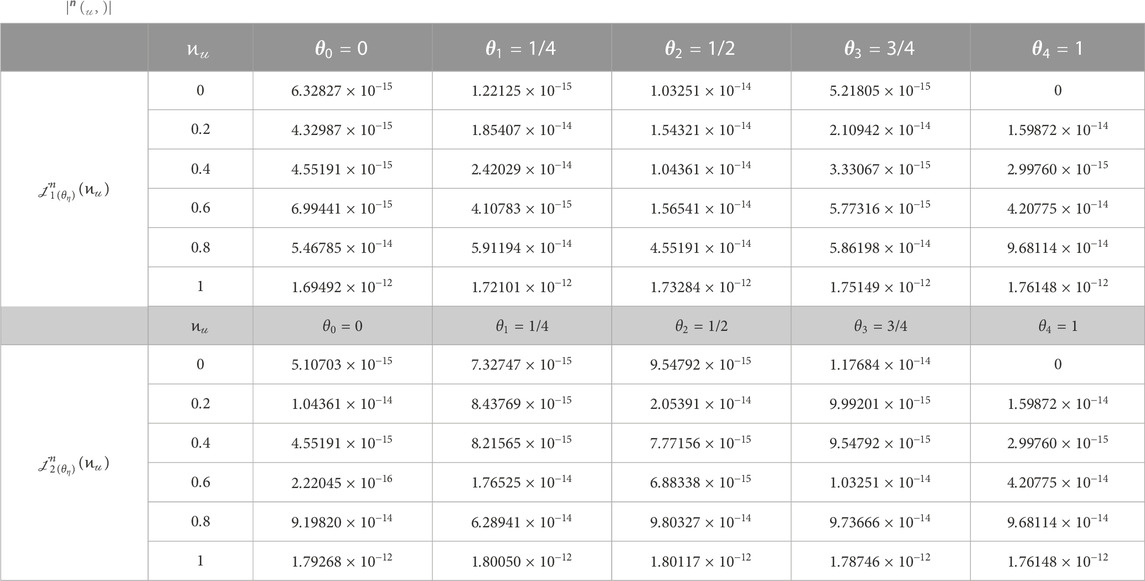
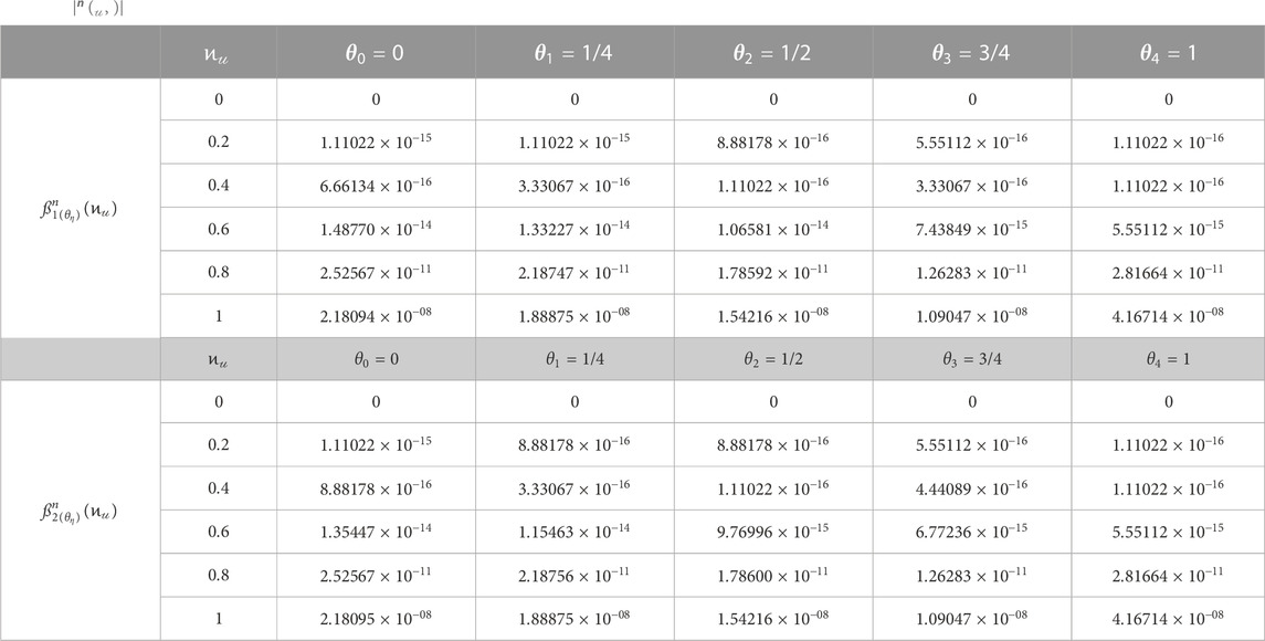
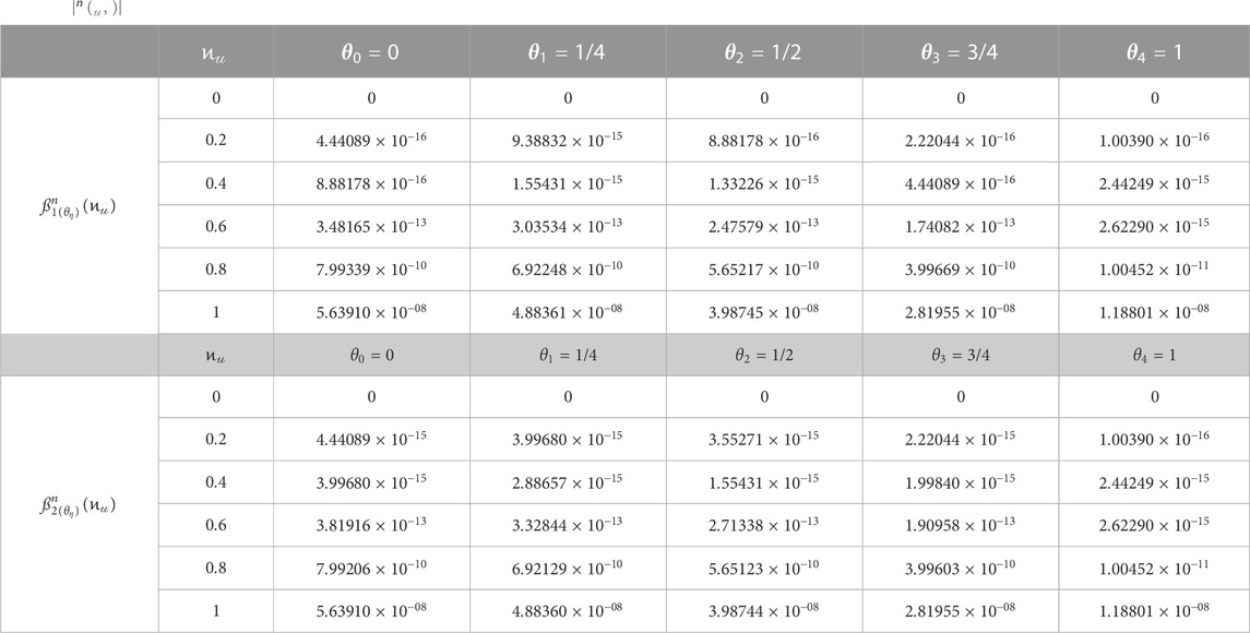
The key goal is to exemplify the uncertain behaviors of the HRKA $\left(1\right)$ - and $\left(2\right)$ -fuzzy M-solutions at dissimilar nodes; Tables 1, 2 show ${ȹ}^n\left({ͷ}_{\mathcal{u}},{\theta }_{\eta }\right)$ in numerically approximating ${\left[{\mathcal{j}}^n\left(ͷ\right)\right]}^{\theta }$ of ${\left[\mathcal{j}\left(ͷ\right)\right]}^{\theta }$ concerning Phase 1 and Phase 2, sequentially in Application 1. Tables 3, 4 show ${ȹ}^n\left({ͷ}_{\mathcal{u}},{\theta }_{\eta }\right)$ in numerically approximating ${\left[{ẞ}^n\left(ͷ\right)\right]}^{\theta }$ of ${\left[ẞ\left(ͷ\right)\right]}^{\theta }$ throughout the HRKA $\left(1\right)$ - and $\left(2\right)$ -fuzzy M-solutions concerning Phase 1 and Phase 2, sequentially in Application 2.

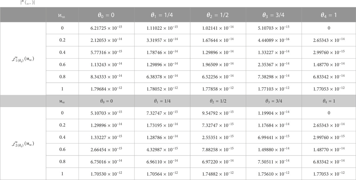
TABLE 1

TABLE 1. $\left|{ȹ}^n\left({ͷ}_{\mathcal{u}},{\theta }_{\eta }\right)\right|$ concerning HRKA $\left(1\right)$ -fuzzy M-solutions for ${\left[{\mathcal{j}}^n\left({ͷ}_{\mathcal{u}}\right)\right]}^{{\theta }_{\eta }}$ in Application 1 in Phase 1 at $\mathfrak{v}=\mathfrak{w}=1$ .

TABLE 2

TABLE 2. $\left|{ȹ}^n\left({ͷ}_{\mathcal{u}},{\theta }_{\eta }\right)\right|$ concerning HRKA $\left(2\right)$ -fuzzy M-solutions for ${\left[{\mathcal{j}}^n\left({ͷ}_{\mathcal{u}}\right)\right]}^{{\theta }_{\eta }}$ in Application 1 in Phase 2 at $\mathfrak{v}=\mathfrak{w}=1$ .

TABLE 3

TABLE 3. $\left|{ȹ}^n\left({ͷ}_{\mathcal{u}},{\theta }_{\eta }\right)\right|$ concerning HRKA $\left(1\right)$ -fuzzy M-solutions for ${\left[{ẞ}^n\left({ͷ}_{\mathcal{u}}\right)\right]}^{{\theta }_{\eta }}$ in Application 2 in Phase 1 at $\mathfrak{v}=\mathfrak{w}=1$ .

TABLE 4

TABLE 4. $\left|{ȹ}^n\left({ͷ}_{\mathcal{u}},{\theta }_{\eta }\right)\right|$ concerning HRKA $\left(2\right)$ -fuzzy M-solutions for ${\left[{ẞ}^n\left({ͷ}_{\mathcal{u}}\right)\right]}^{{\theta }_{\eta }}$ in Application 2 in Phase 2 at $\mathfrak{v}=\mathfrak{w}=1$ .

As is evident from the tabulated digits in Tables 1–4, ${\mathcal{j}}_{1\left({\theta }_{\eta }\right)}^n\left({ͷ}_{\mathcal{u}}\right)\left({ẞ}_{1\left({\theta }_{\eta }\right)}^n\left({ͷ}_{\mathcal{u}}\right)\right)$ and ${\mathcal{j}}_{2\left({\theta }_{\eta }\right)}^n\left({ͷ}_{\mathcal{u}}\right)\left({ẞ}_{2\left({\theta }_{\eta }\right)}^n\left({ͷ}_{\mathcal{u}}\right)\right)$ correspond to the HRKA solutions ${\mathcal{j}}_{1\theta }\left(ͷ\right)\left({ẞ}_{1\theta }\left(ͷ\right)\right)$ and ${\mathcal{j}}_{2\theta }\left(ͷ\right)\left({ẞ}_{2\theta }\left(ͷ\right)\right)$ and are harmonized and approximately similar in their behavior. The tabulated digits in Tables 3, 4 satisfy the property that ${ẞ}_{1\theta }^n\left(ͷ\right)=-{ẞ}_{2\theta }^n\left(ͷ\right)$ for each $\theta$ and $ͷ$ in the two phases to agree the natural constraint appears in Eq. 74 as ${\left[Ɯ\right]}^{\theta }=\left[-\sqrt{1-\theta },\sqrt{1-\theta }\right]$ . Altogether, the HRKA aligns well with the numerical results, indicating a high level of agreement between them.

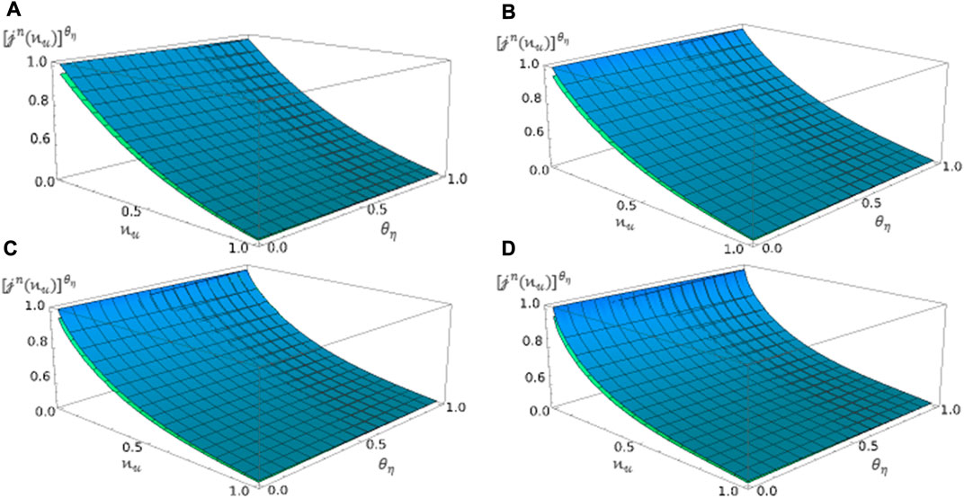
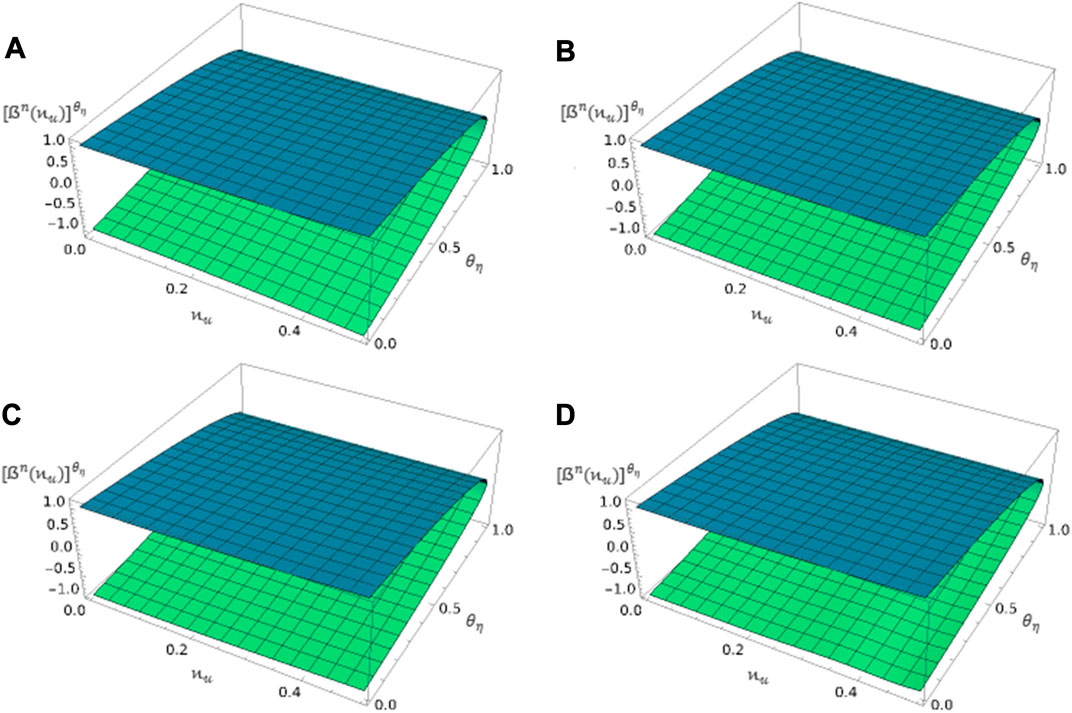
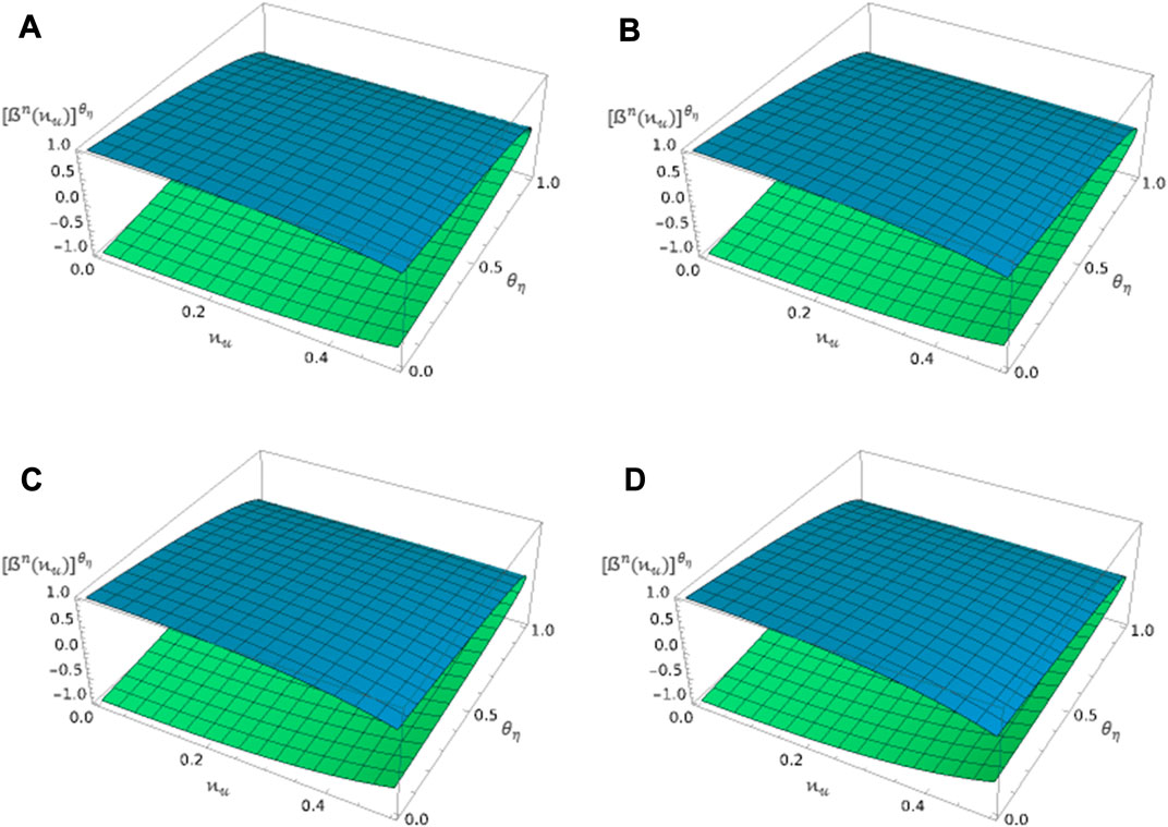
Our research focuses on exploring the HRKA’s vibrant and structural characteristics, and remembrance and heritage features. In pursuit of this, we provide geometric certifications for ${ͷ}_{\mathcal{u}}$ and ${\theta }_{\eta }$ at $\mathfrak{v}\in \mathbb{D}$ , $\mathfrak{w}>0$ , and $\theta \in \mathbb{I}$ . Figures 2, 3 display the HRKA $\left(1\right)$ - and $\left(2\right)$ -fuzzy M-solutions in the phase of $\left\{\mathfrak{v}\left(1\right),\mathfrak{w}\right\}$ and $\left\{\mathfrak{v}\left(2\right),\mathfrak{w}\right\}$ -fuzzy FM-D concerning Application 1. Likewise, Figures 4, 5 exhibit similar computations concerning Application 2.

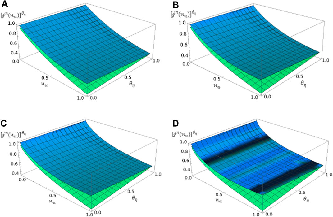
FIGURE 2

FIGURE 2. Plot of HRKA $\left(1\right)$ - and $\left(2\right)$ -fuzzy M-solutions ${\left[{\mathcal{j}}^n\left({ͷ}_{\mathcal{u}}\right)\right]}^{{\theta }_{\eta }}$ in Application 1 in the phase of $\left\{\mathfrak{v}\left(1\right),\mathfrak{w}\right\}$ -fuzzy FM-D: (A) at $\left\{\mathfrak{v},\mathfrak{w}\right\}=\left\{\mathrm{1,1}\right\}$ , (B) at $\left\{\mathfrak{v},\mathfrak{w}\right\}=\left\{\mathrm{0.9,1}\right\}$ , (C) at $\left\{\mathfrak{v},\mathfrak{w}\right\}=\left\{\mathrm{0.8,1}\right\}$ , and (D) at $\left\{\mathfrak{v},\mathfrak{w}\right\}=\left\{\mathrm{0.7,1}\right\}$ . Herein, green represents ${\mathcal{j}}_{1\left({\theta }_{\eta }\right)}^n\left({ͷ}_{\mathcal{u}}\right),$ and blue represents ${\mathcal{j}}_{2\left({\theta }_{\eta }\right)}^n\left({ͷ}_{\mathcal{u}}\right)$ .

FIGURE 3

FIGURE 3. Plot of HRKA $\left(1\right)$ - and $\left(2\right)$ -fuzzy M-solutions ${\left[{\mathcal{j}}^n\left({ͷ}_{\mathcal{u}}\right)\right]}^{{\theta }_{\eta }}$ in Application 1 in the phase of $\left\{\mathfrak{v}\left(2\right),\mathfrak{w}\right\}$ -fuzzy FM-D: (A) at $\left\{\mathfrak{v},\mathfrak{w}\right\}=\left\{\mathrm{1,1}\right\}$ , (B) at $\left\{\mathfrak{v},\mathfrak{w}\right\}=\left\{\mathrm{0.9,1}\right\}$ , (C) at $\left\{\mathfrak{v},\mathfrak{w}\right\}=\left\{\mathrm{0.8,1}\right\}$ , and (D) at $\left\{\mathfrak{v},\mathfrak{w}\right\}=\left\{\mathrm{0.7,1}\right\}$ . Herein, green represents ${\mathcal{j}}_{1\left({\theta }_{\eta }\right)}^n\left({ͷ}_{\mathcal{u}}\right)$ and blue represents ${\mathcal{j}}_{2\left({\theta }_{\eta }\right)}^n\left({ͷ}_{\mathcal{u}}\right)$ .

FIGURE 4

FIGURE 4. Plot of HRKA $\left(1\right)$ - and $\left(2\right)$ -fuzzy M-solutions ${\left[{\mathcal{j}}^n\left({ͷ}_{\mathcal{u}}\right)\right]}^{{\theta }_{\eta }}$ in Application 2 in the phase of $\left\{\mathfrak{v}\left(1\right),\mathfrak{w}\right\}$ -fuzzy FM-D: (A) at $\left\{\mathfrak{v},\mathfrak{w}\right\}=\left\{\mathrm{1,1}\right\}$ , (B) at $\left\{\mathfrak{v},\mathfrak{w}\right\}=\left\{\mathrm{0.9,1}\right\}$ , (C) at $\left\{\mathfrak{v},\mathfrak{w}\right\}=\left\{\mathrm{0.8,1}\right\}$ , and (D) at $\left\{\mathfrak{v},\mathfrak{w}\right\}=\left\{\mathrm{0.7,1}\right\}$ . Herein, green represents ${ẞ}_{1\left({\theta }_{\eta }\right)}^n\left({ͷ}_{\mathcal{u}}\right)$ and blue represents ${ẞ}_{2\left({\theta }_{\eta }\right)}^n\left({ͷ}_{\mathcal{u}}\right)$ .

FIGURE 5

FIGURE 5. Plot of HRKA $\left(1\right)$ - and $\left(2\right)$ -fuzzy M-solutions ${\left[{\mathcal{j}}^n\left({ͷ}_{\mathcal{u}}\right)\right]}^{{\theta }_{\eta }}$ in Application 2 in the phase of $\left\{\mathfrak{v}\left(2\right),\mathfrak{w}\right\}$ -fuzzy FM-D: (A) at $\left\{\mathfrak{v},\mathfrak{w}\right\}=\left\{\mathrm{1,1}\right\}$ , (B) at $\left\{\mathfrak{v},\mathfrak{w}\right\}=\left\{\mathrm{0.9,1}\right\}$ , (C) at $\left\{\mathfrak{v},\mathfrak{w}\right\}=\left\{\mathrm{0.8,1}\right\}$ , and (D) at $\left\{\mathfrak{v},\mathfrak{w}\right\}=\left\{\mathrm{0.7,1}\right\}$ . Herein, green represents ${ẞ}_{1\left({\theta }_{\eta }\right)}^n\left({ͷ}_{\mathcal{u}}\right)$ and blue represents ${ẞ}_{2\left({\theta }_{\eta }\right)}^n\left({ͷ}_{\mathcal{u}}\right)$ .

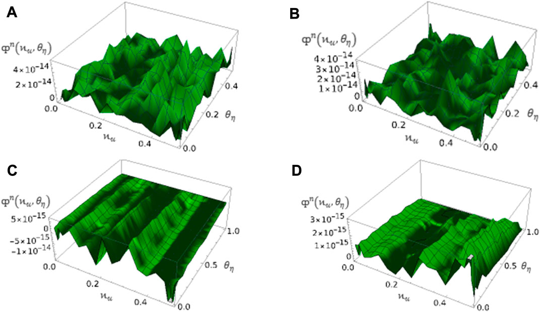
Ultimately, we provide ${ȹ}^n\left({ͷ}_{\mathcal{u}},{\theta }_{\eta }\right)$ geometric certifications for ${ͷ}_{\mathcal{u}}$ and ${\theta }_{\eta }$ at $\mathfrak{v}\in \mathbb{D}$ , $\mathfrak{w}>0$ , and $\theta \in \mathbb{I}$ as visualized in Figure 6 for targeted cases and applications concerning the HRKA $\left(1\right)$ - and $\left(2\right)$ -fuzzy M-solutions in the phase of $\left\{\mathfrak{v}\left(1\right),\mathfrak{w}\right\}$ and $\left\{\mathfrak{v}\left(2\right),\mathfrak{w}\right\}$ -fuzzy FM-D.

FIGURE 6

FIGURE 6. Plot of ${ȹ}^n\left({ͷ}_{\mathcal{u}},{\theta }_{\eta }\right)$ at $\left\{\mathfrak{v},\mathfrak{w}\right\}=\left\{\mathrm{1,1}\right\}$ gained from HRKA $\left(1\right)$ - and $\left(2\right)$ -fuzzy M-solutions: (A) in Application 1 in the phase of $\left\{\mathfrak{v}\left(1\right),\mathfrak{w}\right\}$ -fuzzy FM-D, (B) in Application 1 in the phase of $\left\{\mathfrak{v}\left(2\right),\mathfrak{w}\right\}$ -fuzzy FM-D, (C) in Application 2 in the phase of $\left\{\mathfrak{v}\left(1\right),\mathfrak{w}\right\}$ -fuzzy FM-D, and (D) in Application 2 in the phase of $\left\{\mathfrak{v}\left(2\right),\mathfrak{w}\right\}$ -fuzzy FM-D.

Based on the obtained plots, it is evident that the graphs demonstrate close agreement and similar behaviors, especially when analyzing the classical derivative. It is important to take note that the model profiles can exhibit unusual behaviors when the value of $\left\{\mathfrak{v},\mathfrak{w}\right\}$ deviates from the classical value as fuzzy FM-D can have a significant impact on the results.

9 Key points and summary

In this exploration research, FM-D, FM-I, and FM-FIDM are examined and analyzed for the first time. Alongside, the existence-uniqueness of fuzzy two M-solutions jointly with the characterization theorem is employed as pioneering results as well. Indeed, triplet-simulated pseudocodes related to characterizing $\left(1\right)$ - and $\left(2\right)$ -fuzzy M-solutions are given in terms of algorithms. In this approach, the iterative HRKA in a new perspective is fitted and built to attain a series approximation of $\left(1\right)$ - and $\left(2\right)$ -fuzzy M-solutions for a couple of noninteger uncertain real-world models to ratify and attest to the new scheme as pioneering results as well. Thereafter, computational convergence and error analysis together with the series symbolization of fuzzy two M-solutions are inferred. In conclusion, the obtained novel theories and data outcomes demonstrate the fidelity and productivity of our proposed adaptation. This approach can be potently used as a preference scheme in handling assorted types of fractional M-models manifesting in applied physics and nonlinear engineering. Our manuscript provides a valuable contribution to the field and opens up new avenues for future studies. Our future article will talk about the fractional M-models where $\left.\mathfrak{v}ϵ(\mathrm{1,2}\right]$ and $\mathfrak{w}>0$ .

Data availability statement

The original contributions presented in the study are included in the article/Supplementary Material; further inquiries can be directed to the corresponding author.

Author contributions

OA: data curation, investigation, software, methodology, validation, writing–original draft, and writing–review and editing. RM: funding acquisition, investigation, resources, supervision, visualization, and writing–original draft. BM: conceptualization, formal analysis, investigation, project administration, software, and writing–review and editing. All authors contributed to the article and approved the submitted version.

Acknowledgments

The authors would like to express their gratitude to the unknown reviewers for carefully reading the paper and for their helpful comments.

Conflict of interest

The authors declare that the research was conducted in the absence of any commercial or financial relationships that could be construed as a potential conflict of interest.

Publisher’s note

All claims expressed in this article are solely those of the authors and do not necessarily represent those of their affiliated organizations, or those of the publisher, the editors, and the reviewers. Any product that may be evaluated in this article, or claim that may be made by its manufacturer, is not guaranteed or endorsed by the publisher.

Abbreviations

FM-FIDM, fuzzy M-fractional integrodifferential model; CM-FIDM, crisp M-fractional integrodifferential model; HRKA, Hilbert reproducing kernel algorithm; FM-D, fractional M-derivative; FM-I, fractional M-integral; NLDM, nonlinear differential model; IRCC, inductance–resistance–capacitance circuit.

References

1. Chakraverty S, Tapaswini S, Behera D. Fuzzy differential equations and applications for engineers and scientists. USA: CRC Press (2016).

Google Scholar

2. Gomes LT, de Barros LC, Bede B. Fuzzy differential equations in various approache. Germany: Springer (2015).

Google Scholar

3. Rajab N, Ahmed AM, Al-Faour OM. On fuzzy linear integro-deffrential equations of Volterra type: Approximated solutions of fuzzy linear Volterra integro-differential equations. Moldova: LAP LAMBERT Academic Publishing (2013).

Google Scholar

4. Herrmann R. Fractional calculus: An introduction for physicists. Singapore: World Scientific (2014).

Google Scholar

5. Tarasov VE. Fractional dynamics: Applications of fractional calculus to dynamics of particles, fields and media. Germany: Springer (2011).

Google Scholar

6. West BJ. Fractional calculus view of complexity: Tomorrow’s science. UK: Taylor & Francis (2015).

Google Scholar

7. Shabestari MR, Ezzati R, Allahviranloo T. Numerical solution of fuzzy fractional integro-differential equation via two-dimensional Legendre wavelet method. J Intell Fuzzy Syst (2018) 34:2453–65. doi:10.3233/jifs-171707

CrossRef Full Text | Google Scholar

8. Alikhani R, Bahrami F. Global solutions for nonlinear fuzzy fractional integral and integrodifferential equations. Commun Nonlinear Sci Numer Simulation (2013) 18:2007–17. doi:10.1016/j.cnsns.2012.12.026

CrossRef Full Text | Google Scholar

9. Salahshour S, Allahviranloo T, Abbasbandy S. Solving fuzzy fractional differential equations by fuzzy Laplace transforms. Commun Nonlinear Sci Numer Simulation (2012) 17:1372–81. doi:10.1016/j.cnsns.2011.07.005

CrossRef Full Text | Google Scholar

10. Cui M, Lin Y. Nonlinear numerical analysis in the reproducing kernel space. USA: Nova Science (2009).

Google Scholar

11. Berlinet A, Agnan CT. Reproducing kernel Hilbert space in probability and statistics. USA: Kluwer Academic Publishers (2004).

Google Scholar

12. Daniel A. Reproducing kernel spaces and applications. Basel, Switzerland: Springer (2003).

Google Scholar

13. Jiang W, Chen Z. A collocation method based on reproducing kernel for a modified anomalous subdiffusion equation. Numer Methods Partial Differential Equations (2014) 30:289–300. doi:10.1002/num.21809

CrossRef Full Text | Google Scholar

14. Geng FZ, Qian SP, Li S. A numerical method for singularly perturbed turning point problems with an interior layer. J Comput Appl Math (2014) 255:97–105. doi:10.1016/j.cam.2013.04.040

CrossRef Full Text | Google Scholar

15. Akram G, Rehman HU. Solution of fifth order boundary value problem in the reproducing kernel space. Middle East J Scientific Res (2011) 10:191–5.

Google Scholar

16. Akgül A, Bonyah E. Reproducing kernel Hilbert space method for the solutions of generalized Kuramoto–Sivashinsky equation. J Taibah Univ Sci (2019) 13:661–9. doi:10.1080/16583655.2019.1618547

CrossRef Full Text | Google Scholar

17. Akgül A. A novel method for a fractional derivative with non-local and non-singular kernel. Chaos, Solitons and Fractals (2018) 114:478–82. doi:10.1016/j.chaos.2018.07.032

CrossRef Full Text | Google Scholar

18. Akram G, Rehman HU. Numerical solution of eighth order boundary value problems in reproducing Kernel space. Numers (2013) 62:527–40. doi:10.1007/s11075-012-9608-4

CrossRef Full Text | Google Scholar

19. Akram G, Rehman HU. Solutions of a class of sixth order boundary value problems using the reproducing kernel space,. Abstract Appl Anal (2013) 2013:560590. doi:10.1155/2013/560590

CrossRef Full Text | Google Scholar

20. Attia N, Akgül A, Seba D, Nour A, Riaz MB. Reproducing kernel Hilbert space method for solving fractal fractional differential equations. Results Phys (2022) 35:105225. doi:10.1016/j.rinp.2022.105225

CrossRef Full Text | Google Scholar

21. Abu Arqub O. Adaptation of reproducing kernel algorithm for solving fuzzy Fredholm-Volterra integrodifferential equations. Neural Comput Appl (2017) 28:1591–610. doi:10.1007/s00521-015-2110-x

CrossRef Full Text | Google Scholar

22. Hasan S, Maayah B, Bushnaq S, Momani S. A modified reproducing kernel Hilbert space method for solving fuzzy fractional integro-differential equations. Boletim da Sociedade Paranaense de Matemática (2023) 41:1–16. doi:10.5269/bspm.52289

CrossRef Full Text | Google Scholar

23. Yépez-Martínez H, Gómez-Aguilar JF. M-derivative applied to the dispersive optical solitons for the Schrödinger-Hirota equation. The Eur Phys J Plus (2019) 134:93. doi:10.1140/epjp/i2019-12459-7

CrossRef Full Text | Google Scholar

24. Sousa JVDC, Oliveira ECD. On the local M-derivative. Prog Fractional Differ Appl (2018) 4:479–92. doi:10.18576/pfda/040403

CrossRef Full Text | Google Scholar

25. Yépez-Martínez H, Gómez-Aguilar JF. Local M-derivative of order $$\alpha$$ α and the modified expansion function method applied to the longitudinal wave equation in a magneto electro-elastic circular rod. Opt Quan Elect (2018) 50:375. doi:10.1007/s11082-018-1643-5

CrossRef Full Text | Google Scholar

26. Yusuf A, Inc M, Baleanu D. Optical solitons with M-truncated and beta derivatives in nonlinear optics. Front Phys (2019) 7:126. doi:10.3389/fphy.2019.00126

CrossRef Full Text | Google Scholar

27. Sousa JVDC, Oliveira ECD. A new truncated M-fractional derivative type unifying some fractional derivative types with classical properties. Int J Anal Appl (2018) 16:83–96. doi:10.28924/2291-8639-16-2018-83

CrossRef Full Text | Google Scholar

28. Mohammed WW, El-Morshedy M, Moumen A, Ali EE, Benaissa M, Abouelregal AE. Effects of M-truncated derivative and multiplicative noise on the exact solutions of the breaking soliton equation. Symmetry (2023) 15:288. doi:10.3390/sym15020288

CrossRef Full Text | Google Scholar

29. Li C, Dao X, Guo P. Fractional derivatives in complex planes. Nonlinear Anal Theor Methods Appl (2009) 71:1857–69. doi:10.1016/j.na.2009.01.021

CrossRef Full Text | Google Scholar

30. Guariglia E. Fractional calculus, zeta functions and Shannon entropy. Open Access (2021) 19:87–100. doi:10.1515/math-2021-0010

CrossRef Full Text | Google Scholar

31. Ortigueira MD, Rodríguez-Germá L, Trujillo JJ. Complex grünwald–letnikov, liouville, riemann–liouville, and Caputo derivatives for analytic functions. Commun Nonlinear Sci Numer Simulation (2011) 16:4174–82. doi:10.1016/j.cnsns.2011.02.022

CrossRef Full Text | Google Scholar

32. Guariglia E. Riemann zeta fractional derivative-functional equation and link with primes. Adv Difference Equations (2019) 2019:261. doi:10.1186/s13662-019-2202-5

CrossRef Full Text | Google Scholar

33. Závada P. Operator of fractional derivative in the complex plane. Commun Math Phys (1998) 192:261–85. doi:10.1007/s002200050299

CrossRef Full Text | Google Scholar

34. Lin SD, Srivastava HM. Some families of the Hurwitz–Lerch Zeta functions and associated fractional derivative and other integral representations. Appl Math Comput (2004) 154:725–33. doi:10.1016/s0096-3003(03)00746-x

CrossRef Full Text | Google Scholar

35. Podlubny I. Geometric and physical interpretation of fractional integration and fractional differentiation. Fractional Calculus Appl Anal (2004) 5:367–86.

Google Scholar

36. Goetschel R, Voxman W. Elementary fuzzy calculus. Fuzzy Sets Syst (1986) 18:31–43. doi:10.1016/0165-0114(86)90026-6

CrossRef Full Text | Google Scholar

37. Kaleva O. Fuzzy differential equations. Fuzzy Sets Syst (1987) 24:301–17. doi:10.1016/0165-0114(87)90029-7

CrossRef Full Text | Google Scholar