 Eerdun Buhe1†
 Muhammad Rafiullah
 Naveed Anjum
- 1School of Mathematical Sciences, Hohhot University for Nationalities, Inner Mongolia, China
- 2Department of Mathematics, COMSATS University Islamabad, Lahore, Pakistan
- 3Department of Electronics Engineering, Sir Syed University of Engineering and Technology, Karachi, Pakistan
- 4Department of Mathematics, GC University, Faisalabad, Pakistan
Reduction in forest resources due to increasing global warming and population growth is a critical situation the World faces today. As these reserves decrease, it alarms new challenges that require urgent attention. In this paper, we provide a semi-analytical solution to a nonlinear mathematical model that studies the depletion of forest resources due to population growth and its pressure. With the help of the homotopy perturbation method (HPM), we determine an approximate series solution with few perturbation terms, which is one of the essential power of the HPM method. We compare our semi-analytical results with numerical solutions obtained using the Runge-Kutta 4th-order (RK-4) method. Furthermore, we analyze the model’s behaviour and dynamics by changing the parametric coefficients that represent the depletion rate of forest resources and the growth rate of population pressure and present these findings using various graphs.
1 Introduction
The world faces an alarming issue today due to the depletion of forest resources caused by deforestation, fires, illegal logging, and other factors. Many countries will lose their remaining forests by 2030 if this trend continues, according to a recent report [1]. Urgent action is needed to address this challenge, including better coordination and control of the timber industry and communities that depend on the forests [2]. Mathematics provides some powerful tools to tackle such problems with the help of differential equations which can offer a way to solve dynamical systems making them essential to science, engineering and humanity. Some studies have used the mathematical modeling of forest depletion and suggested solutions using various numerical and analytical methods. Gompil et al. [3] proposed numerical and simulated results for a forest depletion model, while Eswari et al. [4] examined the homotopy perturbation method (HPM) to solve the mathematical model for the depletion of forest resources. Nugraheni et al. [5] proposed stability analysis and numerical simulations for a mangrove forest resource dynamical model. Didiharyono and Kasse [6] studied the stability of a mathematical model for deforestation and presented numerical simulations of the system. All these studies offer useful insights into the dynamics of forest resources and propose possible solutions to handle this critical global problem. This paper concentrates on the study of the depletion of forest resources, employing a mathematical model suggested by Misra, Lata, and Shukla [7]. This mathematical model consists of the cumulative density of forest resources, the density of the population, and population pressure, represented by the variables B, N, and P, respectively. In this model, the connection between forest and population density is considered as a prey-predator logistic model. The forest density decreases as housing and development increase, impacting its growth rate. Population pressure growth is proportional to population density in the model [7]. The authors have investigated existence and uniqueness of the global positive solution and provided numerical simulations to study this model. The cumulative density of forests and population size, are modelled using comprehensive equations with dynamic relations similar to a prey-predator system. The model signifies the depletion of forest resources provoked by population growth, reduction of forest areas for expansion purposes and the depletion by the pressure of the population. In addition, the model considers that the increase in population pressure is proportional to population density. This model consists of dimensionless differential equations. The suggested model [7] can be represented as:
where B (0) ≥ 0, N (0) ≥ 0, P (0) ≥ 0 and we define variables and constant coefficients of this model in the following table as.
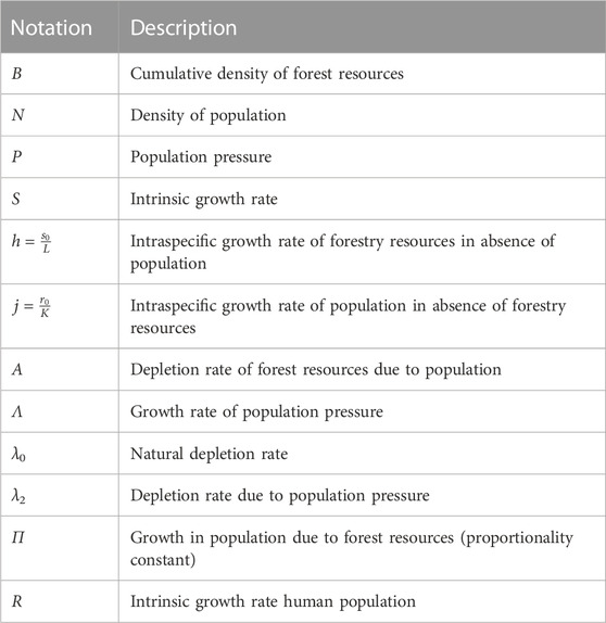
Values for the parameters and coefficients are considered, s = 0.8, s0 = 0.2, L = 50, α = 0.0001, λ = 0.2, λ0 = 0.1, r = 0.2, r0 = 0.1, K = 100, π = 0.004, λ2 = 0.0002,
The rate of forest depletion is alarming, mainly driven by illegal logging and land clearing activities. This trend poses a serious threat to our ecosystem and immediate action is needed to mitigate its impact. Without decisive measures, the depletion of forest resources will have long-lasting consequences on the environment and our wellbeing. It is imperative to find sustainable solutions and enforce regulations to curb the rampant destruction of forests and preserve them for future generations.
Many dynamical problems in science and engineering cannot be solved analytically (exactly) and can be approximated numerically. There is another technique named as series solution (semi-analytical techniques) which is more closer to analytical results. For this purpose a wide range of methods have been developed to find approximate solutions that are as close as possible to the exact solutions. Among these methods are the Taylor series method [8], which approximates functions as power series; the Picard method [9], which iteratively computes solutions from initial conditions; the Adomian decomposition method [10], which decomposes a differential equation into simpler sub problems; the variational iteration method [11], which uses Lagrange multipliers to optimize solutions; and the homotopy perturbation method [12–14,14,15,17–19], which constructs a homotopy that gradually deforms the problem into a simpler one while adding a perturbation term to the solution. These methods have been applied to a wide range of problems in physics, engineering, various fields and have proven to be highly effective in providing accurate approximations to complex dynamical systems.
Ji Huan He, a mathematician from China proposed a novel semi-analytical method based on homotopy and perturbation techniques in 1999, which was named the homotopy perturbation method (HPM) [12]. He improved and extended the HPM to solve a wide range of problems. In 2004, He used the HPM to non-linear oscillators and asymptotic [13,14]. In 2005, the HPM was applied to solve non-linear wave equations and problems related to limit cycle and bifurcation of non-linear systems [15,16]. In 2008, He employed the HPM to solve boundary value problems [20]. In 2007, Javidi and Golbabai used a revised version of the HPM to solve non-linear Fredholm integral equations [21].Recently, HPM with small variations has been applied to study fractal duffing oscillator problems under arbitrary conditions [22], modified HPM for nonlinear oscillators Anjum and He [23], attachment oscillator arising in nanotechnology [24], conservative nonlinear oscillators [25], non-linear oscillator problems in a fractal space [26] and HPM including Aboodh transformation to solve fractional calculus Tao et al. [27], vibrating magnetic inverted pendulum Moatimid et al. [28], Symmetry-breaking and pull-down motion for the helmholtz–duffing oscillator Niu et al. [29], nonlinear fractional Drinfeld–Sokolov–Wilson Equation Nadeem and Alsayaad [30], trajectory analysis of a zero-pitch-angle e-Sail Niccolai et al. [31], natural convection between two concentric horizontal circular cylinders Abdulameer and Ali Al-Saif [32], nonlocal initial-boundary value problems for parabolic and hyperbolic Al-Hayani and Younis [33], multi-step iterative methods for solving nonlinear equations Saeed et al. [34], telegraph equation Moazzzam et al. [35], triangular linear diophantine fuzzy system of equations Shams et al. [36], condensing coagulation model and Lifshitz-Slyzov equation Arora et al. [37], singular nonlinear system of boundary value problems Pathak et al. [38], rikitake-yype system Ene and Pop [39], heat and mass transfer with 2D unsteady squeezing viscous flow problem Abdul-Ameer and Ali Al-Saif [40], variable Speed Wind Turbine Control Shalbafian and Ganjefar [41], radial thrust problem Niccolai et al. [42], special third grade fluid flow with viscous dissipation effect over a stretching sheet Swain et al. [43], and the frequency–amplitude relationship of a nonlinear oscillator with cubic and quintic nonlinearities He et al. [44]. The HPM has become a widely-used technique to solve a large variety of problems in different fields and many research papers have been published each year using this method as evidenced by a simple search on Google Scholar.
In this paper, we provide an approximate solution of model 1) by using the homotopy perturbation method. The interesting feature of HPM is that it provides the best approximate solution by taking a few numbers of perturbation terms.
2 Homotopy perturbation method
Consider a non-linear differential equation
subject to the boundary condition
where D is a differential operator, β is boundary operator, Γ is the boundary of the domain ℧ and g(τ) is an unknown function. The D, generally consist on two parts, linear and non-linear part, represented as L and N respectively. Therefore, 2) can be written as follows
using homotopy method, by taking an embedding parameter q one can construct a homotopy v (τ, q): ℧ × [0, 1] → R for Eq. 4 which satisfies
and it is equivalent to
where q ∈ [0, 1] is an embedding parameter, μ0 is an initial guess approximation of Eq. 6 which satisfies the initial (or boundary) conditions. It can be written as follows.
We suppose the solution in the form of power series for Eq. 5 by taking an embedding parameter q
The approximate solution of Eq. 2 can be obtained by setting q = 1,
The convergence of (Eq. 10) has been proved in [12]. The series is convergent for most cases, however, the convergent rate depends upon the nonlinear operator N(w). Furthermore He suggested the following conditions.
1. The second derivative of nonlinear operator N(w) with respect to w must be small, because the parameter q may be relatively large, i.e., q → 1.
2. The norm of
3 Application of HPM
Now we apply HPM on our model, Eq. 1 of depletion of forest resources (non-linear system of differential equations) as
The initial guesses for (11) are constant as defined in [7].
and we assume the solution of (11) as,
by substituting Eq. 13 in Eq. 11 and collecting the terms of powers of q, we obtain
Now considering s = 0.8, s0 = 0.2, L = 50, α = 0.0001, λ = 0.2, λ0 = 0.1, r = 0.2, r0 = 0.1, K = 100, π = 0.004, λ2 = 0.0002,
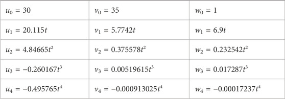
By substituting these values in Eq. 13, we have the solution of model 1) as
For α = 0.0001, α = 0.0002 and α = 0.0004, we have.
B(t)α=0.0001 = 30 + 20.115t + 4.84665t2 − 0.260167t3 − 0.495765t4 + ⋯,
B(t)α=0.0002 = 30 + 20.01t + 4.77438t2 − 0.274268t3 − 0.49119t4 + ⋯ and.
B(t)α=0.0004 = 30 + 19.8t + 4.63094t2 − 0.301744t3 − 0.481988t4 + ⋯.
For λ = 0.1, λ = 0.2 and λ = 0.3, we have.
B(t)λ=0.1 = 30 + 20.115t + 5.16165t2 + 0.0854419t3 − 0.336328t4 + ⋯,
B(t)λ=0.2 = 30 + 20.115t + 4.84665t2 − 0.260167t3 − 0.495765t4 + ⋯ and.
B(t)λ=0.3 = 30 + 20.115t + 4.53165t2 − 0.605776t3 − 0.648587t4 + ⋯.
For λ2 = 0.0001, λ2 = 0.0002 and λ2 = 0.0003, we have.
3.1 Verification of the solution
To verify the validity of solution, first we check the solution for initial conditions which are satisfied at t = 0, secondly we put the solution and its derivatives in the system. If both sides of system are satisfied then we consider the solution is correct or true. For the second condition, we differentiate Eqs 19–21 with respect to t, so we have
Now using Eqs 19–24 and the values of given parameters in system 1) and we have
The coefficients of t powers in Eqs 25–27 are around 15 to 19 decimal places correct to zero. So our series solution (5th degree polynomials) satisfies the system up to 4th degree polynomial (where the coefficients are approximately 17 decimal correct to zero). The solution can be improved by taking/adding more terms of power t in it.
3.2 Results and discussions
In this section, we demonstrate the performance of our model 1 through the evaluation of our calculated approximate solutions, B(t), N(t), and P(t). To validate our results, we compare them with the Runge-Kutta 4th-order method and present the absolute error, eB(t), eN(t), and eP(t) in Table 1 for various time steps. The time domain of our Homotopy Perturbation Method (HPM) is divided into sub-intervals and mapped onto 0 ≤ t ≤ 400 with a step size of 0.5 for graphical representation. Our analysis revealed an average absolute error of 6.53290554e − 08, 5.09269781e − 10, and 1.35452205e − 11 for B(t), N(t), and P(t), respectively. In Tables 2–4, we present the cumulative density of forest resources, B(t), for various values of α, λ, and λ2. These results underscore the versatility and accuracy of our proposed model, which has the potential to contribute significantly to the field of forest resource management. Figure 1 provides a clear illustration of the behaviour of the cumulative density of forest resources B(t), the density of population pressure P(t), and the density of population N(t) as calculated using HPM and RK-4th order method. The solid lines represent the HPM series solution, while the dotted lines show the numerical solution calculated by the RK-4th order method. The graph highlights that the cumulative density of forest resources decreases as the density of population pressure increases. This suggests that controlling population pressure is essential for preserving forests on a large scale. Additionally, Figure 2 depicts the behaviour of model 1 in 3D with respect to HPM and RK method, providing a comprehensive view of the model’s behaviour over time. Figure 3, represents the impact of the depletion rate of forest resources due to population, α = a, on the cumulative density of forest resources, B(t). It reflects that decreasing the depletion rate of forest resources due to population directs to a growth in the cumulative density of forest resources over time. This emphasizes the significance of controlling the population pressure on forests to control their depletion. In Figure 4, we discuss the impact of the growth rate coefficient of population pressure caused by population λ = l on the cumulative density of forest resources B(t). The graph indicates that if we decrease the value of λ, the cumulative density of forest resources increases. Likewise, Figure 5 describes the effect of population pressure λ2 on B(t). We can see, as the value of λ2 decreases, the cumulative density of forest resources B(t) increases. These figures illustrate the significance of controlling population pressure and growth rates to save and preserve forest resources. It also emphasizes the necessity for procedure interventions to control population growth and decrease the depletion of forest resources.
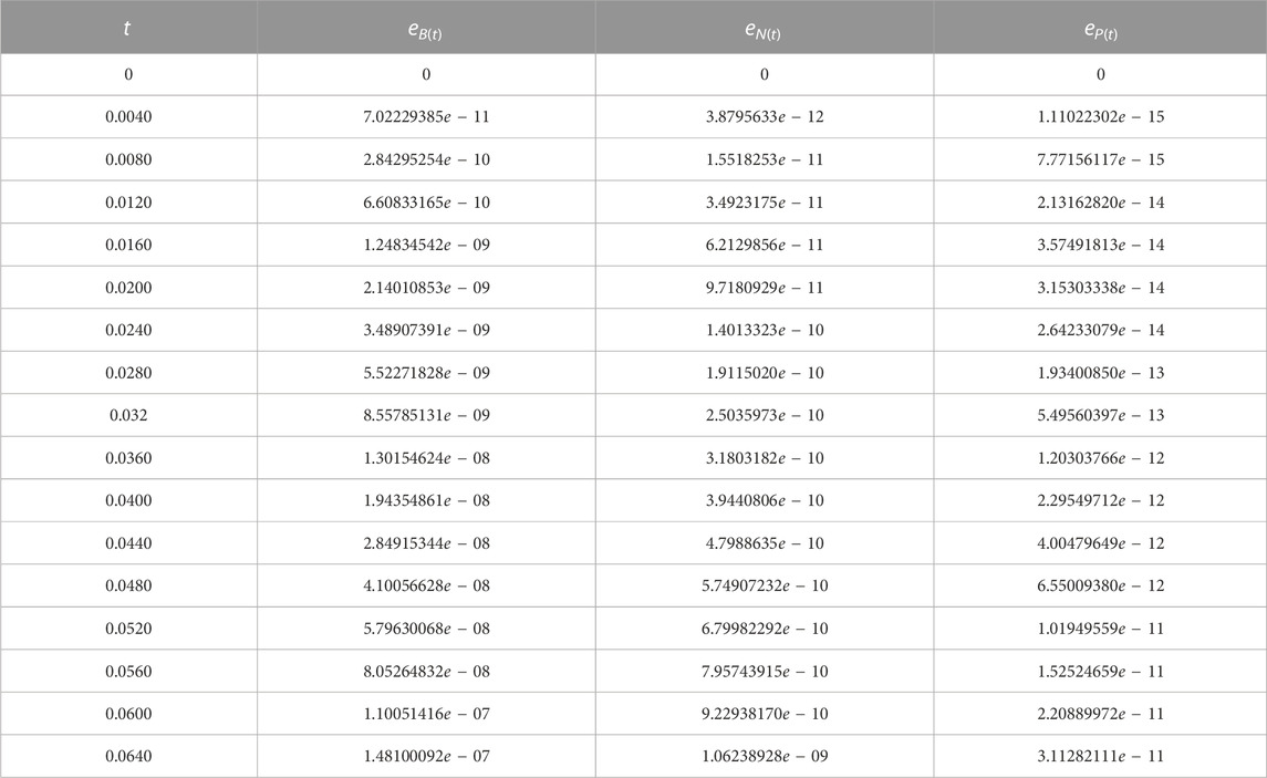
TABLE 1. Error in B(t), N(t) and P(t) by using HPM and RK 4th order.
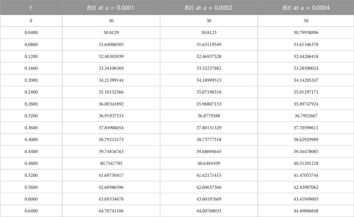
TABLE 2. B(t) by using HPM with variation of α.
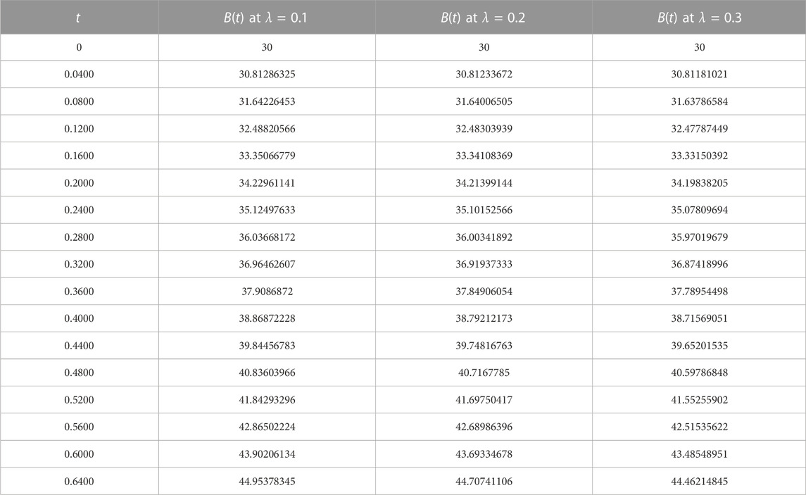
TABLE 3. B(t) by using HPM with variation of λ.
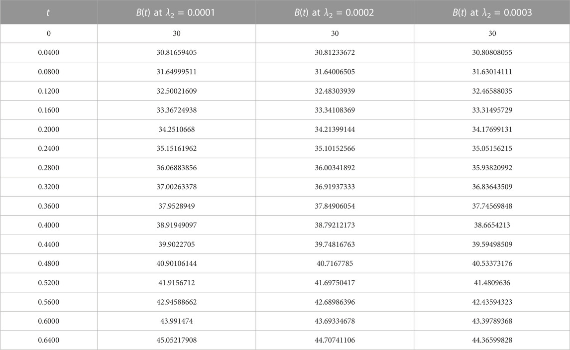
TABLE 4. B(t) by using HPM with variation of λ2.
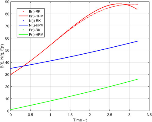
FIGURE 1. Solution for model 1.
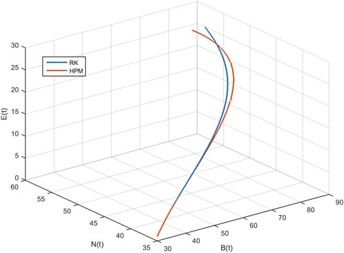
FIGURE 2. Solution for model 1 in 3D.
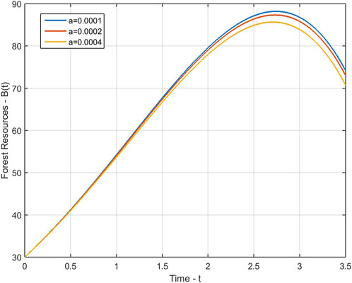
FIGURE 3. Forest resources B(t) and α with the variation of time.
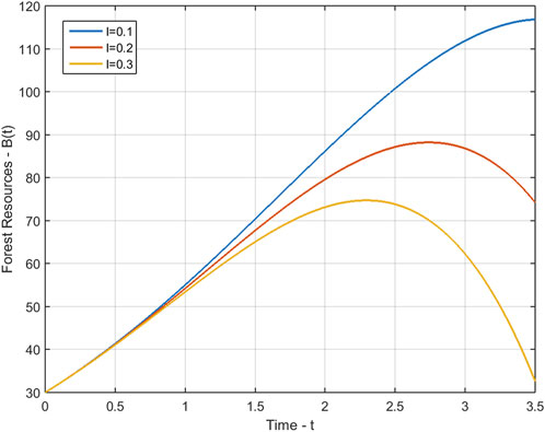
FIGURE 4. Forest resources B(t) and λ with the variation of time.
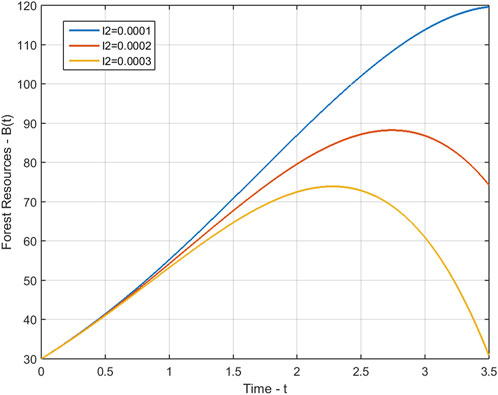
FIGURE 5. Forest resources B(t) and λ2 with the variation of time.
3.3 Technical specification
These calculations are performed on Mathematica® 11.3.0.0 (64-bit) and Matlab® R2015a (8.5.0.197613) 64-bit using a machine Intel(R) Core(TM) i3.2310M CPU @ 2.10 GHz and OS: window 7 Professional (64-bit).
4 Conclusion
In this paper, we used the homotopy perturbation method to obtain a semi-analytical solution for the nonlinear model of the depletion of forest resources. Important characteristic of HPM is that it provides the adequate approximate series solution by taking a few number of perturbation terms which is near to analytical exact solution. Through comparison with the Runge-Kutta method, we established the effectiveness and accuracy of the proposed method. Additionally, we investigated the behaviour of the model by varying the values of the depletion rate of forest resources due to population α, the growth rate coefficient of population pressure caused by population λ, and the depletion rate of its carrying capacity due to population pressure λ2. The results showed that reducing these coefficients can increase the cumulative density of forest resources B(t). These findings highlight the urgent need for measures to conserve forest resources for the wellbeing of our planet. The presented model and its solution indicate the seriousness of this global issue which needs to be acted upon immediately and effectively to preserve our forest resources. This study suggests that additional investigations and research is needed to build more relevant models for assistance of forest resource experts.
Data availability statement
The original contributions presented in the study are included in the article/Supplementary material, further inquiries can be directed to the corresponding authors.
Author contributions
All authors listed have made a substantial, direct, and intellectual contribution to the work and approved it for publication.
Conflict of interest
The authors declare that the research was conducted in the absence of any commercial or financial relationships that could be construed as a potential conflict of interest.
Publisher’s note
All claims expressed in this article are solely those of the authors and do not necessarily represent those of their affiliated organizations, or those of the publisher, the editors and the reviewers. Any product that may be evaluated in this article, or claim that may be made by its manufacturer, is not guaranteed or endorsed by the publisher.
References
1. Asongu SA, Jingwa BA. Population growth and forest sustainability in africa. Int J Green Econ (2012) 6:145–66. doi:10.1504/ijge.2012.050353
2. Ndoye O, Tieguhong JC. Forest resources and rural livelihoods: the conflict between timber and non-timber forest products in the Congo basin. Scand J For Res (2004) 19:36–44. doi:10.1080/14004080410034047
3. Gompil B, Tseveen B, Almasbek J. Modeling and control of Mongolian forest utilization: impact of illegal logging. Nat Resource Model (2022) 35:e12333. doi:10.1111/nrm.12333
4. Eswari A, Kumar SS, Raj SV, Priya VS Analysis of mathematical modeling the depletion of forestry resource: effects of population and industrialization. Matrix Sci Mathematic (Msmk) (2019) 3:22–6. doi:10.26480/msmk.02.2019.22.26
5. Nugraheni K, Burhan M, Pancahayani S, Azka M. Stability analysis of mangrove forest resource depletion models due to the opening of fish pond land. In: Journal of physics: conference series, 1277. IOP Publishing (2019).012037.
6. Didiharyono D, Kasse I. Mathematical modelling of deforestation due to population density and industrialization. Jurnal Varian (2021) 5:9–16. doi:10.30812/varian.v5i1.1412
7. Misra A, Lata K, Shukla J. Effects of population and population pressure on forest resources and their conservation: a modeling study. Environ Dev sustainability (2014) 16:361–74. doi:10.1007/s10668-013-9481-x
8. Corliss G, Chang Y. Solving ordinary differential equations using taylor series. ACM Trans Math Softw (Toms) (1982) 8:114–44. doi:10.1145/355993.355995
9. Picard É. Sur l’application des méthodes d’approximations successives à l’étude de certaines équations différentielles ordinaires. J de mathématiques pures appliquées (1893) 9:217–71.
10. Adomian G. Solving frontier problems of physics: the decomposition method, 60. Springer Science and Business Media (2013).
11. Wu Y, He JH. Variational principle for the Kaup-Newell system. J. comput. appl. mech. (2023) 54 (3):405–409. doi:10.22059/JCAMECH.2023.365116.875
12. He J-H. Homotopy perturbation technique. Comp Methods Appl Mech Eng (1999) 178:257–62. doi:10.1016/s0045-7825(99)00018-3
13. He J-H. The homotopy perturbation method for nonlinear oscillators with discontinuities. Appl Math Comput (2004) 151:287–92. doi:10.1016/s0096-3003(03)00341-2
14. He J-H. Asymptotology by homotopy perturbation method. Appl Maths Comput (2004) 156:591–6. doi:10.1016/j.amc.2003.08.011
15. He J-H. Limit cycle and bifurcation of nonlinear problems. Chaos, Solitons and Fractals (2005) 26:827–33. doi:10.1016/j.chaos.2005.03.007
16. He J-H. Application of homotopy perturbation method to nonlinear wave equations. Chaos, Solitons and Fractals (2005) 26:695–700. doi:10.1016/j.chaos.2005.03.006
17. Rafiullah M, Rafiq A. A new approach to solve systems of second order non-linear ordinary differential equations. Acta Universitatis Apulensis Mathematics-informatics (2010) 24:189–200.
18. Rafiq A, Rafiullah M. Some new multi-step iterative methods for solving nonlinear equations using modified homotopy perturbation method. Nonlinear Anal Forum (2008) 13:185–94.
19. Chakraverty S, Mahato N, Karunakar P, Rao TD. Advanced numerical and semi-analytical methods for differential equations. John Wiley and Sons (2019).
20. He J. Homotopy perturbation method for solving boundary value problems. Phisical Lett (2006) 350:87–8. doi:10.1016/j.physleta.2005.10.005
21. Javidi M, Golbabai A. Modified homotopy perturbation method for solving non-linear fredholm integral equations. Chaos, Solitons and Fractals (2009) 40:1408–12. doi:10.1016/j.chaos.2007.09.026
22. He JH, Jiao ML, He CH Homotopy perturbation method for fractal duffing oscillator with arbitrary conditions. FRACTALS (fractals) (2022) 30:1–10. doi:10.1142/s0218348x22501651
23. Anjum N, He J-H. Two modifications of the homotopy perturbation method for nonlinear oscillators. J Appl Comput Mech (2020) 6:1420–5. doi:10.22055/JACM.2020.34850.2482
24. Ali M, Anjum N, Ain QT, He J-H. Homotopy perturbation method for the attachment oscillator arising in nanotechnology. Fibers Polym (2021) 22:1601–6. doi:10.1007/s12221-021-0844-x
25. Anjum N, He J-H. Higher-order homotopy perturbation method for conservative nonlinear oscillators generally and microelectromechanical systems’ oscillators particularly. Int J Mod Phys B (2020) 34:2050313. doi:10.1142/s0217979220503130
26. He J-H, Moatimid GM, Zekry MH. Forced nonlinear oscillator in a fractal space. Facta Universitatis, Ser Mech Eng (2022) 20:001–20. doi:10.22190/fume220118004h
27. Tao H, Anjum N, Yang Y-J. The aboodh transformation-based homotopy perturbation method: new hope for fractional calculus. Front Phys (2023) 11:310. doi:10.3389/fphy.2023.1168795
28. Moatimid GM, Amer T, Zekry MH. Analytical and numerical study of a vibrating magnetic inverted pendulum. Archive Appl Mech (2023) 93:2533–47. doi:10.1007/s00419-023-02395-3
29. Niu J-Y, He C-H, Alsolami AA. Symmetry-breaking and pull-down motion for the helmholtz–duffing oscillator. J Low Frequency Noise, Vibration Active Control (2023). doi:10.1177/14613484231193261
30. Nadeem M, Alsayaad Y. A new study for the investigation of nonlinear fractional drinfeld–sokolov–wilson equation. Math Probl Eng (2023) 2023:1–9. doi:10.1155/2023/9274115
31. Niccolai L, Quarta AA, Mengali G, Bassetto M. Trajectory analysis of a zero-pitch-angle e-sail with homotopy perturbation technique. J Guidance, Control Dyn (2023) 46:734–41. doi:10.2514/1.g007219
32. Abdulameer YA, Ali Al-Saif AJ. Analytical simulation of natural convection between two concentric horizontal circular cylinders: a hybrid fourier transform-homotopy perturbation approach. Math Model Eng Probl (2023) 10:886–96. doi:10.18280/mmep.100319
33. Al-Hayani WM, Younis MT. The homotopy perturbation method for solving nonlocal initial-boundary value problems for parabolic and hyperbolic partial differential equations. Eur J Pure Appl Maths (2023) 16:1552–67. doi:10.29020/nybg.ejpam.v16i3.4794
34. Saeed HJ, Ali AH, Menzer R, Poclean AD, Arora H. New family of multi-step iterative methods based on homotopy perturbation technique for solving nonlinear equations. Mathematics (2023) 11:2603. doi:10.3390/math11122603
35. Moazzzam A, Anjum A, Saleem N, Kuffi EA. Study of telegraph equation via he-fractional laplace homotopy perturbation technique. Ibn Al-haitham J Pure Appl Sci (2023) 36:349–64. doi:10.30526/36.3.3239
36. Shams M, Kausar N, Khan N, Shah MA. Modified block homotopy perturbation method for solving triangular linear diophantine fuzzy system of equations. Adv Mech Eng (2023) 15:168781322311595. doi:10.1177/16878132231159519
37. Arora G, Kumar R, Mammeri Y. Homotopy perturbation and adomian decomposition methods for condensing coagulation and lifshitz-slyzov models. GEM-International J Geomathematics (2023) 14:4. doi:10.1007/s13137-023-00215-y
38. Pathak P, Barnwal AK, Sriwastav N, Singh R, Singh M. An algorithm based on homotopy perturbation theory and its mathematical analysis for singular nonlinear system of boundary value problems. Math Methods Appl Sci (2023). doi:10.1002/mma.9299
39. Ene R-D, Pop N. Semi-analytical closed-form solutions for the rikitake-type system through the optimal homotopy perturbation method. Mathematics (2023) 11:3078. doi:10.3390/math11143078
40. Abdul-Ameer YA, Ali Al-Saif A-SJ. Fourier-homotopy perturbation method for heat and mass transfer with 2d unsteady squeezing viscous flow problem. J Comput Appl Mech (2023) 54:219–35. doi:10.22059/jcamech.2023.356976.817
41. Shalbafian A, Ganjefar S. Variable speed wind turbine control using the homotopy perturbation method. Int J Precision Eng Manufacturing-Green Tech (2023) 10:141–50. doi:10.1007/s40684-022-00422-2
42. Niccolai L, Quarta AA, Mengali G. Application of homotopy perturbation method to the radial thrust problem. Astrodynamics (2023) 7:251–8. doi:10.1007/s42064-022-0150-4
43. Swain S, Swain BK, Sahoo B. Application of homotopy perturbation method on special third grade fluid flow with viscous dissipation effect over a stretching sheet. Int J Mod Phys C (2023) 34:2350060. doi:10.1142/s0129183123500602
Keywords: semi-analytical solution, system of non-linear differential equations, homotopy perturbation method, depletion of forest resources, mathematical mobel
Citation: Buhe E, Rafiullah M, Jabeen D and Anjum N (2023) Application of homotopy perturbation method to solve a nonlinear mathematical model of depletion of forest resources. Front. Phys. 11:1246884. doi: 10.3389/fphy.2023.1246884
Received: 24 June 2023; Accepted: 04 October 2023;
Published: 20 October 2023.
Edited by:
Yusry El-Dib, Ain Shams University, EgyptReviewed by:
Youssri Hassan Youssri, Cairo University, EgyptMuhammad Nadeem, Qujing Normal University, China
Copyright © 2023 Buhe, Rafiullah, Jabeen and Anjum. This is an open-access article distributed under the terms of the Creative Commons Attribution License (CC BY). The use, distribution or reproduction in other forums is permitted, provided the original author(s) and the copyright owner(s) are credited and that the original publication in this journal is cited, in accordance with accepted academic practice. No use, distribution or reproduction is permitted which does not comply with these terms.
*Correspondence: Muhammad Rafiullah, cmFmaXVsbGFoYXJhaW5AZ21haWwuY29t; Naveed Anjum, eHNuYXZlZWRAeWFob28uY29t
†These authors have contributed equally to this work