 Jakob Kjærulff Svaneborg
 Aleksander Bach Lorentzen1
 Mads Brandbyge
95% of researchers rate our articles as excellent or good
Learn more about the work of our research integrity team to safeguard the quality of each article we publish.
Find out more
ORIGINAL RESEARCH article
Front. Phys. , 28 August 2023
Sec. Condensed Matter Physics
Volume 11 - 2023 | https://doi.org/10.3389/fphy.2023.1237383
Terahertz (THz) field pulses can now be applied in scanning tunneling microscopy (THz-STM) junction experiments to study time-resolved dynamics. The relatively slow pulse compared to the typical electronic time-scale calls for approximations based on a time-scale separation. Here, we contrast three methods based on non-equilibrium Green’s functions: i) the steady-state, adiabatic results, ii) the lowest-order dynamic expansion in the time variation, and iii) the auxiliary mode propagation method without approximations in the time variation. We consider a concrete THz-STM junction setup involving a hydrogen adsorbate on graphene where the localized spin polarization can be manipulated on/off by a local field from the tip electrode and/or a back-gate affecting the in-plane transport. We use steady-state non-equilibrium Green’s function theory combined with density functional theory to obtain a Hubbard model for the study of the junction dynamics. Solving the Hubbard model in a mean-field approximation, we find that the near-adiabatic first-order dynamic expansion in the time variation provides a good description for STM voltage pulses up to the 1 V range.
Recently, it has become possible to extend scanning tunneling microscopy (STM) studies to the time domain by applying strong sub-cycle near-field electromagnetic pulses in the THz regime inside the STM, so-called THz-STM.. This enables studies of time-resolved dynamics of the transport in junctions with sub-Å and sub-ps resolution [1–3]. Due to the strong field confinement at the STM tip electrode, the effective voltages between tip and sample can be on the order of 1 V [4].
The STM-THz experiments pose interesting questions regarding the theoretical description of the dynamics of the electronic subsystem on the time scale of typical atomic vibrations. The case of atomic-scale junctions in STM under strong bias and coupling to the tip requires the consideration of coupling to semi-infinite electrodes. To this end, the non-equilibrium Green’s function (NEGF) methods [5–7] have been a popular choice, where the electrodes are included via self-energies. However, it is relevant to consider simplifications to the full time dynamics since the electron dynamics most often nearly adiabatically follow fields in the THz range. This can be accomplished by the Wigner representation, which involves a time-scale separation into a slow THz time scale (T) and a fast electronic time scale (τ), typically around a femtosecond. This has been considered recently by Honeychurch and Kosov [8] where the NEGF Kadanoff–Baym equations (KBEs) are expressed in the so-called Wigner form with an expansion in terms of the derivative of the slow time, T, from hereon called “dynamic expansion” (DE).
From a numerical point of view, one important advantage of the DE approach is that each discrete time step will be independent from each other: quantities like electron density and current are expressed by quantities independent of the other time steps allowing for computational parallelization over time as opposed to the time propagation of the KBEs. This is important for efficient calculations based, e.g., on first-principles methods such as time-dependent density functional theory based on the NEGF (TD-DFT-NEGF).
In this paper, we apply the DE method to a realistic STM junction which has received considerable attention, namely, STM on a hydrogen adsorbate on graphene. This system is magnetic, but the magnetism can be tuned by the applied tip or gate field, resulting in a change in the in-plane spin transport. Here, we will consider the junction subject to a THz pulse and use it to benchmark the DE against the full time-dependent NEGF calculation with the auxiliary mode (AM) method and steady-state field approximation (zero-order DE). We first use steady-state DFT-NEGF to examine the bias- and gate-dependent electronic structure and in-plane transport in the system. We extract parameters from here to obtain an effective mean field, a Hubbard model for the junction, which we use for benchmarking and which serves as a toy model of a full TD-DFT-NEGF calculation, highlighting the numerical considerations in a self-consistent treatment of time-dependence within the DE approach. Our results show how the computationally efficient DE method is able to capture the main features in the THz dynamics of the system, in particular that the THz-bias pulse gives rise to fast switching dynamics of the magnetism, generating higher harmonic dynamics in the occupations and currents which, on the other hand, are not captured well by the steady-state adiabatic approximation.
Magnetism of graphene can be created by point defects like adsorption of isolated hydrogen (H/Gr) or a vacancy, owing to the creation of unpaired π electrons around the defects [9]. The electronic density of graphene is highly tunable by electrostatic gating [10] which makes it interesting to consider how this magnetism may be tunable either by a global back-gate or a local gating such as the voltage on the STM tip, see Figures 1A,B.
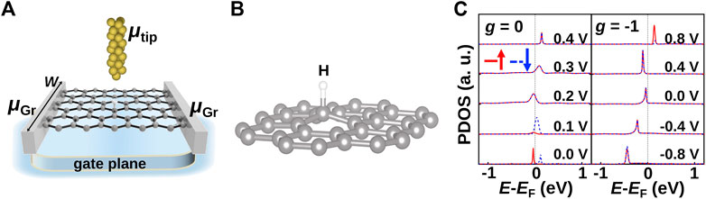
FIGURE 1. (A) Schematic of the three-terminal hydrogen on the graphene (H/Gr) device setup with a charge back-gate plane. μtip and μGr are chemical potentials of the gold tip and graphene electrodes. Here, W is the width of the device. (B) Local atomic structure of the hydrogen atom on graphene showing an out-of-plane buckling of the C atom below H (sp3 hybridization). (C) Density of states projected on the H atom, the midgap states, with g = 0 and g = −1 gating in units of 1013cm−2, respectively. Solid red and dashed blue lines represent spin up and down populations, respectively. EF refers to the Fermi energy of the system in equilibrium, i.e., without bias.
First, we consider steady-state DFT-NEGF calculations where we use a three-terminal device setup with a gate plane, encompassing left and right graphene electrodes (with width W), and an additional gold tip electrode above the H atom, as schematically shown in Figure 1A. The calculations were performed using the SIESTA/TranSIESTA package [11–14] with the GGA-PBE [15] functional for exchange correlation, a DZP atomic orbital basis set and an electronic temperature of 50 K (for further details, see the work of Gao et al. [16]). To model the gate-induced doping of graphene, a gate plane was placed 15 Å underneath the graphene. The gate carries a charge density of n = g × 1013 e/cm2, where g defines the gating level, with g < 0 (g > 0) corresponding to n(p) doping [17].
The local atomic structure of H/Gr in Figure 1B displays an out-of-plane buckling of the C atom, leading to a transition from sp2 to sp3 hybridization. In Figure 1C, we show the calculated density of states around the Fermi energy (EF) projected on the H atom (PDOS) without gating, g = 0, and with gate-induced n-doping, g = −1. The H impurity resonances at the center of the graphene’s pseudogap, the midgap peaks, imply a strong interaction between the s orbital of the H atom and the pz orbital of graphene. Here, the H adatom forms a σ bond with the carbon atom next to it, and π bonds are broken. The bonding states are located at −8 eV, far below the Fermi level.
We use a tip-H distance of 4.5 Å, where there is only a weak connection between the tip and H to keep the spin moment at 1 μB as the initial state at zero bias (0 V) and gate. Without gating, the magnetic moment can be switched on/off with the tip voltage-induced doping below the tip, as observed by the disappearance of the spin splitting in the PDOS. On the other hand, we can also turn the magnetism “off” for an n-doped graphene by applying gating (g = −1), where we see a non-spin split, fully occupied peak for zero tip bias (0 V). In this situation the magnetism/spin splitting reappears when we apply a 0.8 V tip bias counteracting the gate doping. Thus, it is possible to manipulate the spin by either the STM tip bias or by a global field from a gate plane [16]. The main driver for this behavior is the electronic occupation of the carbon below the hydrogen.
Next, we address the effects of the field and spin manipulation on the in-plane transport in H/Gr. To this end, we consider the energy-dependent scattering cross section, σ(E) [18], corresponding to the “shadowing” length (area) caused by the point defect in 2D (3D) conductors. We can estimate σ(E) from the electron transmission functions for the pristine and defected systems, T0 and T, respectively [19, 20].
where W is the width of the device, as shown in Figure 1A. In Figure 2A, we see two peaks around EF caused by the resonant, spin-split H resonances, c.f. the PDOS in Figure 1C, yielding a significant in-plane transport spin polarization, Pσ = (σ↑ − σ↓)/(σ↑ + σ↓). The cross section we obtain here is close to the one obtained for H on graphene nanoribbons [18]. In accordance with the PDOS in Figure 1C, we observe in Figure 2A how the spin splitting and transport spin polarization vanish when applying a tip voltage. On the other hand, as shown in Figure 2B, we show how the in-plane transport spin polarization can be turned “on” using the counteracting tip bias for the gate-induced n-doped system. In this case, we also observe a dip in the cross section around −0.3 eV below EF, corresponding to the Dirac point of the doped graphene substrate. The H resonance is pinned around the Fermi level at equilibrium (0 V), but it can be shifted by the tip bias. This shows how external biases may be used to turn spin polarization “on/off” in the H/Gr system and how this has implications not only for the tunnel current between the tip and sample (PDOS) but also for the in-plane transport in graphene.
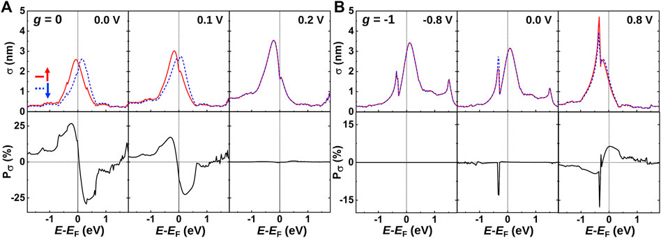
FIGURE 2. In-plane spin-dependent elastic scattering cross section (σ) as a function of energy. In the bottom panel, the corresponding spin polarization (Pσ) without (A) g = 0 and (B) with g =−1 gate-induced n doping is shown. Solid red and dashed blue lines represent spin-up and spin-down states, respectively.
We consider next the response of the H/Gr system to a time-dependent variation of the tip and gate potentials with the waveform shown in Figure 3A chosen to mimic THz pulses in typical experiments [1, 4],
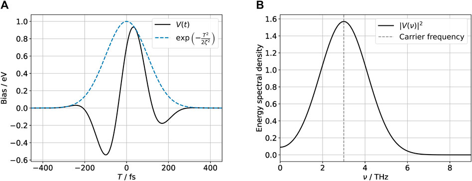
FIGURE 3. THz pulse used to drive the system in the time-domain (A) and frequency domain (B). The pulse has the form
We will use a minimal model for the H/Gr system with parameters chosen according to the aforementioned DFT calculations and model the system in the typical electrode–device–electrode setup where the time-dependence of the potential is considered in the device region, while the electrodes are assumed to be perfectly screened so that the time dependence in these regions consists only of a rigid shift of the energies and chemical potentials following the pulse [5]. The device region consists of the hydrogen atom and the sp3 carbon atom in the graphene on which it is adsorbed. This system is modeled using an electronic two-level model for each spin, corresponding to one orbital per atom per spin. The coupling to the graphene sheet and the STM tip electrodes is included using self-energies. We note that the spin-polarization in the H/Gr in reality involves carbon atoms further away from the adsorbate [9], but we will neglect these effects here.
The system is described by the total Hamiltonian
where
Here, αk is a generalized state label referring to the eigenstates of the isolated graphene sheet and tip, respectively. The mean-field Hubbard Hamiltonian
where
and to the graphene sheet through the C atom on the adsorption site
such that vtip,k is the hopping matrix element between the tip state k and the hydrogen orbital and vgr,k is the hopping matrix element between the graphene state k and the device carbon orbital. These parameters enter the numerical model only indirectly through the electrode self-energies to be specified below.
The values of the model parameters were estimated to mimic the results of the DFT calculation, and we find that the values ɛH = −1.7 eV, ɛC(t) = 0 eV + ΔgrV(t), vCH = 3.25 eV, U = 6.5 eV, Δgr = 1, and Δtip = 0 resulted in a qualitative agreement between the models when comparing PDOS on the respective atoms and their spin splitting. The effect of the THz pulse is to shift the graphene electronic energies relative to the tip. There is no spin-flipping mechanism such that the spin-up and spin-down electrons effectively form two separate systems, interacting only through the time-dependent mean-field occupation of the opposite spin on the H atom, which must be solved self-consistently.
The dynamical evolution of the system for a given time-dependence may be described using the NEGF formalism. We now express all operators as matrices in the device state space, consisting of the hydrogen and carbon orbital for each spin. The retarded, advanced, and lesser Green’s functions in the device region are governed by the KBEs [5],
for the retarded/advanced functions and
for lesser Green’s function. In these equations, Σ = Σgr + Σtip is the self-energy related to the coupling of the device to the graphene sheet and the tip. These self-energies may be found from Green’s function operator gα of the electrodes in the absence of coupling to the device:
In the present work, the tip is modeled in the wide-band limit using an energy constant,
We note that all quantities in Eqs (7) and (8) are matrices in the device state-space. Thus, in our model, we obtain two sets of 2 × 2 matrices, one set for each spin. To solve the KBEs, we use two different numerical approaches. The first is a method based on the separation of time scales [8], where the resulting equations of motion are expanded in an asymptotic series, which we denote as the DE. This represents an approximation to the dynamics, which becomes exact when the external time-dependence varies on a much slower time scale than the electronic degrees of freedom in the system. The second method (AM) recasts the KBEs into a set of coupled ordinary differential equations (ODEs) which depend only on a single time variable. The system dynamics can then be found by propagating these ODE’s forward in time from a specified initial condition [22, 23]. This method provides an exact propagation of the dynamics, but requires that the self-energies be approximated by a series of Lorentzian functions. In the following, we will provide some more details on these two schemes.
We introduce a central time variable T and a difference time variable τ,
In the absence of external driving, the system is invariant with respect to translations in time, and thus, in this case, the quantities in the KBEs will only be a function of the difference time τ. The introduction of an external time-dependent driving breaks time-translation invariance and, thus, introduces a dependence on the central time variable T. Therefore, the variables (T, τ) are well suited to separate the time scales associated with internal dynamics of the system (τ) and the external driving (T). After the introduction of the new time variables, we cast the KBEs in the so-called Wigner space representation by performing a Fourier transform over τ. Thus, we obtain a new set of Green’s functions and self-energies:
where the superscript ∼ indicates that a quantity is in the Wigner representation. After transforming all self-energies and Green’s functions to the Wigner representation, the KBEs of motion take the form
and
where the differential operators in the exponentials act only on the function whose superscript they bear. For notational convenience, we have suppressed the arguments (T, ω) on the self-energies and Green’s functions. We note that Eqs (12) and (13) are still formally exact. If the time-dependence is taken to be adiabatic, all central-time derivatives in Eqs (12) and (13) vanish. In this limit, the exponentials act as the identity operator, and we obtain the well-known steady-state KBEs in the frequency domain:
where the 0 subscripts indicate that these are adiabatic Green’s functions. If we assume that the external perturbation acts on a much slower time scale than any internal dynamics in the system, G and Σ will be slowly varying functions of the central time T. In that case, we can expand the exponential operators in Eqs (12) and (13) and keep only the lowest order terms on the grounds that higher-order terms contain higher powers of the central time derivative ∂T, which must be small by virtue of the slow variation. This allows us to expand the Green’s functions in a formal series.
where Gi satisfies an equation of motion containing terms only of ith order in the central time derivative ∂T. Thus, G0 describes the adiabatic response of the system (Eqs (14)–(15)) to the time-dependent perturbation, while G1 describes the first-order dynamical corrections and so on. The explicit expressions for Gr/a and G< resulting from this expansion at the zeroth and first orders of approximation are shown in Supplementary Material.
Once the Green’s functions governing the system have been found, the time-resolved current into the device from the graphene sheet and tip, respectively, is given by [5]
where the current matrix Cα is
In the Wigner space representation, the integral in Eq. (18) becomes an exponential operator, and we find the equivalent expression in terms of Wigner space quantities as
We expand the current and current matrix in a series in the same manner as we did for the Green’s functions.
where Jα,i = Tr Cα,i, and Cα,i satisfies an equation containing terms of order i in ∂T. These equations, at each order, are found from the series expansion of the exponential operator in Eq. (19) and the expansion Eq. (16) of the Green’s functions by collecting all terms of the same order in ∂T. They are given explicitly in Supplementary Material.
It is worth emphasizing that the method does not require any propagation of the equations of motion because the dynamics are included as time-dependent corrections to the adiabatic solution. It is, therefore, well suited to problems where exact propagation may not be computationally feasible, such as problems that require the consideration of dynamics over very long time scales, and, in particular, the computations may be parallelized trivially over the discrete time steps of the central time variable, T.
The device Hamiltonian is an input parameter to the dynamical expansion and, thus, must be known a priori. This represents a problem for working with systems with interactions or electron–electron repulsion, as the effective device Hamiltonian will then depend on the state of the system. One approach to this problem is the introduction of correlation self-energies, which must then also be approximated by an additional expansion in ∂T [24]. In this work, we use instead an iterative procedure, seeking a self-consistent dynamical electron density. This approach is in the spirit of DFT, and we envision that future implementations of the method may work with DFT programs to obtain self-consistent dynamical corrections to time-dependent problems. In our approach, we start from a self-consistent adiabatic solution on a pre-defined time-grid. The self-consistent adiabatic Hamiltonian obtained from this solution is then used as the input Hamiltonian to the DE model, from which a new dynamical Hamiltonian is obtained on the same time grid. This process is repeated until the self-consistency of the dynamical Hamiltonian is achieved. Obtaining convergence for all time steps is not trivial except at very low frequencies ν0 of the external perturbation and was not obtained at the highest frequencies investigated. This is related to the fact that the higher-order harmonics generated by the switching of the magnetization state are highly non-adiabatic and, therefore, unsuitable for description by an expansion such as the DE. Nonetheless, for frequencies below ν0 ≈ 5 THz, the dynamical corrections were in good agreement with the exact time propagation (AM) scheme even when the self-consistent cycle did not formally converge for all time steps. Further details of the numerical implementation may be found in Supplementary Material.
The KBE, as shown in Eq. 8, can be dealt with under the assumption that the spin-independent electrode broadening matrices
with a corresponding retarded self-energy
In Eq. (21), Wαl is a fitting coefficient in a matrix sense, and in Eq. (22),
where the current matrix Cα is defined in Eq. (18)
The memory integral is handled through contour integration and identifying so-called auxiliary modes to obtain the auxiliary mode approach to the problem [23]. The current matrix Cα(t) has several associated equations of motion with coefficients related to the weights and poles in Eq. (21) (23). The system of ODEs, as shown in Eq. (23), can then be solved using a standard ODE solver method. In this particular case, an adaptive Runge–Kutta–Fehlberg fourth-order method (RKF45) was used [31]. This serves as a basis for comparison, as this method is only dependent on having a suitable fit of Γα instead of having an approximation of how fast the system can change. Because of the setup, getting the fit of Γα for each electrode is just fitting two scalar functions to the form in Eq. (21), which is easily carried out using an equally spaced grid and minimizing the least square error with respect to the fitting coefficient on each Lorentzian.
These steps, from obtaining fits to the lead Γα’s to propagating the density matrix and its auxiliary modes in time in a numerically exact way, were implemented in a code that will be published in the future. The fits used can be seen in Figure 4A together with a comparison of the transmission function (tip to graphene) with numerically “exact” self-energies and fitted self-energies in Figure 4B. For the fits, as shown in Figure 4, 100 Lorentzians were used.
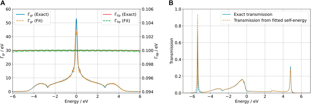
FIGURE 4. (A) Lorentzian fits to Γgr (blue) and Γtip (red) used for the AM approach. (B) Tip-graphene transmission function calculated with the numerically “exact” self-energies and the fitted Γ’s without the Hubbard term (U = 0). The transmission was calculated using TBtrans [13].
To test our methods, we calculate self-consistently the time-dependent occupation of spin-up and spin-down electrons on the H atom and central C atom, along with the time-resolved spin-polarized current injected into the graphene sheet. A net current may be injected since electrons can tunnel from the STM tip through the hydrogen atom and into the graphene sheet. These properties are calculated using the two methods outlined previously. For our purposes, the AM method may be regarded as numerically exact. In the DE method, the equations of motion are expanded to first order; i.e., we include only first-order dynamical corrections. In the fully adiabatic limit, the self-consistent solution to the electronic dynamics may be found semi-analytically, and for comparison, we include such a calculation in all figures shown.
In the absence of the THz pulse, the system relaxes to an equilibrium configuration which is similar to the ground-state found in the DFT calculations in Section 3. In particular, the ground state is spin polarized when VDC = 0, but the polarization vanishes upon the inclusion of a sufficiently large bias. We analyze in the following the dynamics for VDC = 0.5 eV and VDC = 0.0 eV. These two situations correspond to the situations in the top (0.4 V) and bottom (0.0 V) panels in the left (g = 0) part of Figure 1C, respectively. This way of applying a DC bias to the system mimics that used in the experiment by Cocker et al. [32].
In Figure 5, we show the time-dependent occupation of the hydrogen (A and B) and carbon (C and D) orbitals as determined self-consistently by the DE and the AM method when the system is perturbed by the THz pulse. We take the central frequency of the pulse to be ν0 = 3 THz and its amplitude to 1 eV, as shown in the experiment by Peller et al. [4]. We will show in the following that the DE method breaks down for this system between 5 and 10 THz, and so 3 THz is one of the highest frequencies for which we would expect the method to work. The gray dotted line marks the adiabatic self-consistent solution, which neglects all dynamics associated with the finite response time of the electronic system. The main new feature when dynamics are included is a delay in the switching time from the polarized to the non-polarized state, and vice versa. The DE and AM methods are in reasonably good agreement with respect to this time delay, in particular for the polarized → non-polarized (P → NP) transition for the DC biased system in Figures 5A,C. Note that for the NP → P transition to occur, the spin-up/down symmetry of the system must be spontaneously broken. Physically, this is achieved by any random (e.g., thermal) fluctuation of the system, but in the numerical implementation, a small spin-up/down asymmetry is introduced explicitly to break this symmetry. We implemented this by introducing a small energy splitting between spin-up and -down electrons, ɛH → ɛH + ɛσ, where ɛ↑/↓ = ∓1 μeV, i.e., a much smaller energy scale than any other scales in the system. This parameter, therefore, controls the spontaneous symmetry breaking during the NP → P transition without, otherwise, affecting the dynamics.
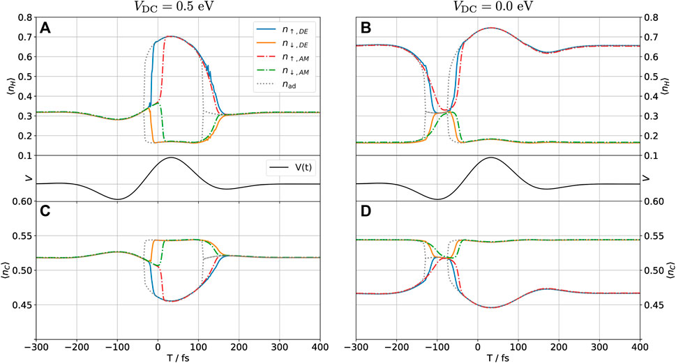
FIGURE 5. (A) Time-dependent occupation of the hydrogen orbital (⟨nH⟩(t)) as determined self-consistently by the DE and the AM method when the system is perturbed by a THz pulse at a central frequency of 3 THz (middle panels) for a DC bias where the system is non-polarized (VDC = 0.5 eV). (B) H-occupation for a DC bias yielding a polarized system (VDC = 0 eV). (C) Carbon pz-orbital occupation (⟨nC⟩(t)) for non-polarized and (D) polarized cases. In each case, the lines labeled nad mark the adiabatic solution to the problem.
The sign of ɛσ was chosen to make the system eventually return to the initial polarization state for the unbiased configuration. One could equally well have chosen the opposite sign, which would make the pulse switch the polarization state of the H adatom for sufficiently low central frequencies. In the absence of an external magnetic field splitting the degeneracy between the spin states and if the central frequency of the pulse is sufficiently low to completely quench the polarization, the final polarization state would be independent of the initial state.
In Figure 5C, we can observe that as the hydrogen atom acquires a spin polarization, the carbon atom acquires the reverse polarization. This happens even though the model does not include electron–electron repulsion in the carbon orbital. It is known that the spin polarization of a hydrogen adsorbate on graphene induces a sublattice-dependent spin polarization in the graphene, extending for several unit cells around the adsorption site [9, 16]. Our observation is qualitatively in line with these results, though the effect could be modeled more accurately by using a spin-dependent coupling self-energy for the graphene-device contact. One could also include more carbon atoms in the device region and, thus, explicitly model their time-dependent spin polarization. The AM results for the carbon orbital were shifted by a constant vertical off-set to make all methods agree in the steady-state regime. If such an offset is not included, a small discrepancy is observed due to the Lorentzian fit to the self-energy used in the AM method in place of the exact self-energy. The carbon orbital, which couples directly to the graphene sheet through the self-energy, is particularly sensitive to any variation in this parameter. We remark that the quality of the fit may always be improved by including more Lorentzian functions, until a satisfactory fit is achieved.
Figure 6 shows the time-resolved spin-polarized current Js = J↑ − J↓ injected into the graphene due to the THz pulse for the DC biased and unbiased configurations. Large peaks are observed when the magnetization state switches, corresponding to the abrupt change in occupation of the hydrogen atom. These peaks are completely absent in the adiabatic calculation. The DE result displays rapid small-amplitude oscillations shortly before the switch occurs. This is a numerical artifact which reflects the fact that the self-consistent cycle did not converge for these particular time steps. This is not surprising as the DE approach is based on the assumption that the time-evolution is near adiabatic, which is far from the case near the transition, see the discussion in Supplementary Material. Despite this challenge, the overall prediction by the DE method is in good agreement with the exact (AM) result, especially for the biased (NP → P → NP) configuration.
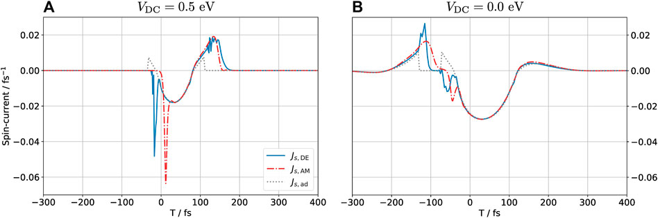
FIGURE 6. Spin-polarized current Js = J↑− J↓ into the graphene layer for (DC) biased (A) and unbiased (B) configurations. A positive sign of Js means that there is a net spin-up current into the graphene sheet. Both time-dependent methods predict large spikes in the current when the polarization state of the hydrogen atom changes, in particular during the transition from non-polarized to polarized currents. This feature is absent in the adiabatic calculation.
The spectrum of the spin-polarized current is shown in Figure 7. The DE and AM spin-polarized currents contain significant Fourier components at much higher frequencies than the adiabatic current, as one may have anticipated from the peaks observed in Figure 6. They both also predict oscillations in the spectra at high frequencies (most evident in Figure 7A), although the amplitudes and exact locations of these oscillations are different. This finding indicates that the DE method captures well the qualitative effects of the dynamics, but it may not be quantitatively correct on all accounts. All three methods predict currents whose spectra contain higher frequencies than the incident THz pulse, attesting to the highly non-linear behavior of the system.
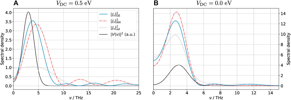
FIGURE 7. Spectrum of the spin-polarized current Js = J↑ − J↓ into the graphene layer for (DC) biased (A) and unbiased (B) configurations. Due to the spike in the current associated with the spin-polarization phase transition, the spectrum of the current contains much larger frequencies than that of the external pulse, an indication that the problem is highly non-linear. This is especially evident in the biased case, when the non-polarized → polarized transition is particularly rapid. Note the different scales of both axes in the two figures; the black curve showing the spectrum of the external pulse in arbitrary units is the same in both figures.
As the DE method is exact in the adiabatic limit, a natural question is how fast the externally imposed time-dependence may be before the method breaks down. Figure 8 shows the total spin injected into the graphene sheet
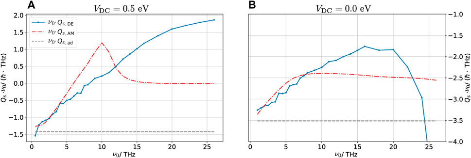
FIGURE 8. Total spin injected into the graphene layer multiplied by pulse frequency plotted for various frequencies for (DC) biased (A) and unbiased (B) configurations. The total spin injected is calculated as
Neglecting dynamical effects (i.e., the adiabatic case), the transferred spin is inversely proportional to the central frequency of the pulse because the current is frequency-independent. To highlight the difference due to the dynamical corrections, we plot ν0Qs which is constant for the adiabatic calculation and is shown in Figure 8 as a gray dashed line. At low frequencies, the DE and AM methods are in good agreement, predicting that the transferred charge is roughly independent of ν0, which is observed in Figure 8 as a linear relationship between ν0Qs and ν0. At low frequency, the system has time to completely polarize/depolarize, resulting in an approximately frequency-independent current associated with the filling and emptying of the device orbitals. As the frequency increases the DE method begins to deviate. From the figures, we assess that ν0 ≈ 5 THz is the largest frequency for which the DE works well. We remark that at high frequencies, the self-consistent cycle used in the DE method does not converge well. For these frequencies, the dynamical density with the smallest error obtained in the self-consistent cycle is included in the figure. The dots show the frequencies at which calculations were made, and the lines interpolate between these points. In the biased case (Figure 8A), the dynamical behavior predicted by the AM method changes significantly around ν0 = 10 THz. This change is related to the fact that at high frequencies, the electronic system cannot adjust to follow the pulse. Thus, when the system starts out in the NP state, it does not have time to polarize. For a fully non-polarized system, the spin-polarized charge will always vanish due to the spin-up/down symmetry. This explains the sudden decrease in the transferred charge at this point. This highly non-adiabatic effect is not at all captured by the DE method.
We have tested the computationally efficient DE/time-scale separation method, introduced in [8] on a model of an experimentally relevant system, namely, mean-field, open-system calculations of charge, and spin dynamics in a THz-STM junction involving a hydrogen adsorbate on graphene. We demonstrated that for low THz frequencies, the DE method gives a good description of the non-adiabatic dynamics compared to full propagation using the AM method. This calculation may, furthermore, be seen as a toy model for a self-consistent TD-DFT-NEGF setup, where dynamical corrections to the density due to an external field are taken into account via the dynamical expansion method. Some of the numerical challenges and methods are discussed in Supplementary Material.
We have shown how the THz pulse generates spin-dynamics in the hydrogen on the graphene THz-STM system with higher harmonic frequencies appearing due to the highly non-linear system. This dynamics may affect both the tunnel current from the tip electrode as well as the spin-dependent scattering of carriers in graphene, as observed by the spin-dependent scattering cross section of the hydrogen adsorbate.
The magnetic structure in the graphene induced by the polarized hydrogen atom is long ranged [9]. As an outlook, it would be interesting to extend the computational region and possibly to include dynamics among multiple localized spins. We also note that the carrier-envelope phase (CEP) may be changed so the THz waveform changes in a continuous way, e.g., from maximum being positive to negative [33], as a further way of tuning the dynamics.
The expansion in powers of the central time derivative ∂T used in the DE may in principle be continued up to arbitrary order to include dynamical effects to higher degrees of accuracy. It would be interesting to extend the numerical implementation beyond the first-order dynamical corrections. In a preliminary study, we found that it was difficult to converge the self-consistent cycle within the second-order DE, and we did not pursue this further. An open question for the DE method is the issue of convergence. It is not trivial to quantify how slow the external time variation in a given system should be in order for the lowest-order terms to approximate the full dynamics. A further investigation into this issue would be highly interesting, in particular, in combination with the inclusion of higher-order terms in the formal series expansion.
The raw data supporting the conclusions of this article will be made available by the authors, without undue reservation.
JKS implemented the DE method and performed the DE and some of the AM calculations. ABL implemented the AM method and performed some of the AM calculations. FG performed the DFT-NEGF calculations. All authors contributed to the article and approved the submitted version.
JKS, FG were supported by Villum fonden (Project No. VIL 13340), ABL by the Independent Research Fund Denmark (Project No. 0135-00372A), and APJ by the Center for Nanostructured Graphene (CNG), which is sponsored by the Danish National Research Foundation (Project No. DNRF103).
The authors thank Profs. Peter Uhd Jepsen and Peter Bøggild for stimulating discussions.
The authors declare that the research was conducted in the absence of any commercial or financial relationships that could be construed as a potential conflict of interest.
All claims expressed in this article are solely those of the authors and do not necessarily represent those of their affiliated organizations, or those of the publisher, the editors, and the reviewers. Any product that may be evaluated in this article, or claim that may be made by its manufacturer, is not guaranteed or endorsed by the publisher.
The Supplementary Material for this article can be found online at: https://www.frontiersin.org/articles/10.3389/fphy.2023.1237383/full#supplementary-material
1. Ammerman SE, Jelic V, Wei Y, Breslin VN, Hassan M, Everett N, et al. Lightwave-driven scanning tunnelling spectroscopy of atomically precise graphene nanoribbons. Nat Commun (2021) 12:6794. doi:10.1038/s41467-021-26656-3
2. Cocker TL, Jelic V, Hillenbrand R, Hegmann FA. Nanoscale terahertz scanning probe microscopy. Nat Photon (2021) 15:558–69. doi:10.1038/s41566-021-00835-6
3. Wang L, Xia Y, Ho W. Atomic-scale quantum sensing based on the ultrafast coherence of an h2 molecule in an stm cavity. Science (2022) 376:401–5. doi:10.1126/science.abn9220
4. Peller D, Roelcke C, Kastner LZ, Buchner T, Neef A, Hayes J, et al. Quantitative sampling of atomic-scale electromagnetic waveforms. Nat Photon (2021) 15:143–7. doi:10.1038/s41566-020-00720-8
5. Haug H, Jauho AP. Quantum kinetics in transport and optics of semiconductors. Berlin, Germany: Springer (2008).
6. Stefanucci G, Van Leeuwen R. Nonequilibrium many-body theory of quantum systems: a modern introduction. Cambridge, United Kingdom: Cambridge University Press (2013).
8. Honeychurch TD, Kosov DS. Timescale separation solution of the Kadanoff-Baym equations for quantum transport in time-dependent fields. Phys Rev B (2019) 10:245423. doi:10.1103/PhysRevB.100.245423
9. González-Herrero H, Gómez-Rodríguez JM, Mallet P, Moaied M, Palacios JJ, Salgado C, et al. Atomic-scale control of graphene magnetism by using hydrogen atoms. Science (2016) 352:437–41. doi:10.1126/science.aad8038
10. Novoselov KS, Geim AK, Morozov SV, Jiang D, Zhang Y, Dubonos SV, et al. Electric field effect in atomically thin carbon films. Science (New York, N.Y.) (2004) 306:666–9. doi:10.1126/science.1102896
11. Brandbyge M, Mozos JL, Ordejón P, Taylor J, Stokbro K. Density-functional method for nonequilibrium electron transport. Phys Rev B (2002) 65:165401. doi:10.1103/physrevb.65.165401
12. Soler JM, Artacho E, Gale JD, García A, Junquera J, Ordejón P, et al. The siesta method for ab initio order-n materials simulation. J Phys Condensed Matter (2002) 14:2745–79. doi:10.1088/0953-8984/14/11/302
13. Papior N, Lorente N, Frederiksen T, García A, Brandbyge M. Improvements on non-equilibrium and transport green function techniques: the next-generation transiesta. Comp Phys Commun (2017) 212:8–24. doi:10.1016/j.cpc.2016.09.022
15. Perdew JP, Burke K, Ernzerhof M. Generalized gradient approximation made simple. Phys Rev Lett (1996) 77:3865–8. doi:10.1103/physrevlett.77.3865
16. Gao F, Zhang Y, He L, Gao S, Brandbyge M. Control of the local magnetic states in graphene with voltage and gating. Phys Rev B (2021) 103:L241402. doi:10.1103/PhysRevB.103.L241402
17. Papior N, Gunst T, Stradi D, Brandbyge M. Manipulating the voltage drop in graphene nanojunctions using a gate potential. Phys Chem Chem Phys (2016) 18:1025–31. doi:10.1039/c5cp04613k
18. Saloriutta K, Uppstu A, Harju A, Puska MJ. Ab initio transport fingerprints for resonant scattering in graphene. Phys Rev B (2012) 86:235417. doi:10.1103/physrevb.86.235417
19. Markussen T, Rurali R, Cartoixa X, Jauho AP, Brandbyge M. Scattering cross section of metal catalyst atoms in silicon nanowires. Phys Rev B (2010) 81:125307. doi:10.1103/physrevb.81.125307
20. Uppstu A, Saloriutta K, Harju A, Puska M, Jauho AP. Electronic transport in graphene-based structures: an effective cross-section approach. Phys Rev B (2012) 85:041401. doi:10.1103/physrevb.85.041401
21. Papior N, Calogero G, Leitherer S, Brandbyge M. Removing all periodic boundary conditions: efficient nonequilibrium green’s function calculations. Phys Rev B (2019) 100:195417. doi:10.1103/physrevb.100.195417
22. Croy A, Saalmann U. Propagation scheme for nonequilibrium dynamics of electron transport in nanoscale devices. Phys Rev B - Condensed Matter Mater Phys (2009) 80:245311. doi:10.1103/PhysRevB.80.245311
23. Popescu BS, Croy A. Efficient auxiliary-mode approach for time-dependent nanoelectronics. New J Phys (2016) 18:093044. doi:10.1088/1367-2630/18/9/093044
24. Kershaw VF, Kosov DS. Non-equilibrium Green’s function theory for non-adiabatic effects in quantum transport: inclusion of electron-electron interactions. J Chem Phys (2019) 150:074101. doi:10.1063/1.5058735
25. Xie H, Jiang F, Tian H, Zheng X, Kwok Y, Chen S, et al. Time-dependent quantum transport: an efficient method based on liouville-von-neumann equation for single-electron density matrix. J Chem Phys (2012) 137:044113. doi:10.1063/1.4737864
26. Zheng X, Chen G, Mo Y, Koo S, Tian H, Yam C, et al. Time-dependent density functional theory for quantum transport. J Chem Phys (2010) 133:114101. doi:10.1063/1.3475566
27. Zheng X, Wang F, Yam CY, Mo Y, Chen G. Time-dependent density-functional theory for open systems. Phys Rev B (2007) 75:195127. doi:10.1103/physrevb.75.195127
28. Jauho AP, Wingreen NS, Meir Y. Time-dependent transport in interacting and noninteracting resonant-tunneling systems. Phys Rev B (1994) 50:5528–44. doi:10.1103/physrevb.50.5528
29. Hu J, Luo M, Jiang F, Xu RX, Yan Y. Padé spectrum decompositions of quantum distribution functions and optimal hierarchical equations of motion construction for quantum open systems. J Chem Phys (2011) 134:244106. doi:10.1063/1.3602466
30. Jin J, Zheng X, Yan Y. Exact dynamics of dissipative electronic systems and quantum transport: hierarchical equations of motion approach. J Chem Phys (2008) 128:234703. doi:10.1063/1.2938087
31. Hairer E, Nørsett SP, Wanner G. Solving ordinary differential equations. 1, Nonstiff problems. Berlin, Germany: Springer-Vlg (1993).
32. Cocker TL, Peller D, Yu P, Repp J, Huber R. Tracking the ultrafast motion of a single molecule by femtosecond orbital imaging. Nature (2016) 539:263–7. doi:10.1038/nature19816
Keywords: THz spin-electronics, time-dependent transport, graphene magnetism, non-equilibrium Green’s functions, Wigner representation, density functional theory–non-equilibrium Green’s function
Citation: Svaneborg JK, Bach Lorentzen A, Gao F, Jauho A-P and Brandbyge M (2023) Manipulation of magnetization and spin transport in hydrogenated graphene with THz pulses. Front. Phys. 11:1237383. doi: 10.3389/fphy.2023.1237383
Received: 09 June 2023; Accepted: 07 August 2023;
Published: 28 August 2023.
Edited by:
Hang Xie, Chongqing University, ChinaReviewed by:
Jianbao Zhao, Canadian Light Source, CanadaCopyright © 2023 Svaneborg, Bach Lorentzen, Gao, Jauho and Brandbyge. This is an open-access article distributed under the terms of the Creative Commons Attribution License (CC BY). The use, distribution or reproduction in other forums is permitted, provided the original author(s) and the copyright owner(s) are credited and that the original publication in this journal is cited, in accordance with accepted academic practice. No use, distribution or reproduction is permitted which does not comply with these terms.
*Correspondence: Mads Brandbyge, bWFickBkdHUuZGs=
Disclaimer: All claims expressed in this article are solely those of the authors and do not necessarily represent those of their affiliated organizations, or those of the publisher, the editors and the reviewers. Any product that may be evaluated in this article or claim that may be made by its manufacturer is not guaranteed or endorsed by the publisher.
Research integrity at Frontiers
Learn more about the work of our research integrity team to safeguard the quality of each article we publish.