
94% of researchers rate our articles as excellent or good
Learn more about the work of our research integrity team to safeguard the quality of each article we publish.
Find out more
ORIGINAL RESEARCH article
Front. Phys., 21 July 2023
Sec. Interdisciplinary Physics
Volume 11 - 2023 | https://doi.org/10.3389/fphy.2023.1216451
This article is part of the Research TopicAnalytical Methods for Nonlinear Oscillators and Solitary WavesView all 14 articles
 Farah M. Al-Askar1†
 Wael W. Mohammed2,3*†
Here, we look at the Sasa-Satsuma equation with M-truncated derivative (SSE-MTD). The analytical solutions in the form of trigonometric, hyperbolic, elliptic, and rational functions are constructed using the Jacobi elliptic function and generalizing Riccati equation mapping methods. Because the Sasa–Satsuma equation is applied to explain the propagation of femtosecond pulses in optical fibers, the acquired solutions can be employed to explain a wide range of important physical phenomena. Moreover, we apply the MATLAB tool to generate a series of graphs to address the effect of the M-truncated derivative on the exact solution of the SSE-MTD.
Many authors have centered their attention on fractional nonlinear differential equations (FNLDEs) in the noble age of technology and science to examine complex mathematical models that are used in research area and real life, such as neuroscience, robotics, fluid dynamics, quantum mechanics, plasma physics, optical fibers, and so on. A lot studies have been published about some aspects of fractional differential equations, such as finding exact and numerical solutions, the existence and uniqueness of solutions, and the stability of solutions [1–7]. Therefore, it is essential to discover the exact solutions to these equations in order to understand the physical phenomenon and overcome the resulting obstacles. Recently, acquiring soliton solutions to important equations has emerged as a major field of study. Numerous researchers defended numerous novel methods to evaluate soliton solutions including (G′/G, 1/G)-expansion method [8] (G′/G)-expansion [9, 10], generalized (G′/G)-expansion [11], exp-function method [12], Jacobi elliptic function expansion [13], sine-cosine procedure [14], auxiliary equation scheme [15], first-integral method [16], sine-Gordon expansion technique [17], generalized Kudryashov approach [18], exp(−ϕ(ς))-expansion method [19], homotopy perturbation method with Aboodh transform [20], He–Laplace method, He’s variational iteration method [21, 22], and others.
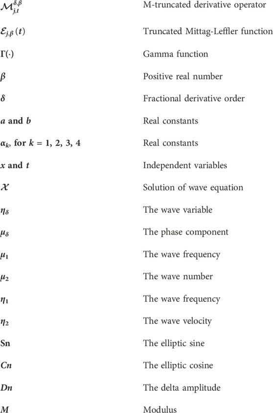
In contrast, a new differentiation operator has grown up, that includes the concepts of fractional differentiation and fractal derivative. Therefore, various kinds of fractional derivatives were proposed by several mathematicians. The most well-known ones are the ones proposed by Grunwald-Letnikov, He’s fractional derivative, Atangana-Baleanu’s derivative, Riemann-Liouville, Marchaud, Riesz, Caputo, Hadamard, Kober, and Erdelyi [23–26]. The bulk of fractional derivative types do not follow classic derivative equations like the chain rule, quotient rule, and product rule. Sousa et al. [27] have developed a new derivative known as the M-truncated derivative (MTD), which is a natural extension of the classical derivative. The MTD for
where
The MTD has the following characteristics for any real integers a and b [27]:
(1)
(2)
(3)
(4)
(5)
There are many authors have considered some nonlinear partial differential equations with M-truncated derivative such as [28–31] and the references therein. In this article, we examine the Sasa-Satsuma equation with M-truncated derivative (SSE-MTD):
where
If we set δ = 1 and β = 0, then we have the Sasa-Satsuma (SS) equation (32, 33):
The SS Eq. 2, which was found while studying the integrability of Schrödinger equation, reduced to nonlinear Schrödinger equation when α1 = α2 = α3 = 0 as follows:
In 1991, Sasa and Satsuma [34] created Eq. 2. This equation has additional components that explain third-order dispersion, self-steepening, and self-frequency shift, which are prevalent in many areas of physics, such as ultrashort pulse propagation in optical fibers [35, 36]. Due to the importance of SS Eq. 2, many authors have obtained its exact solutions by using various methods such as new auxiliary equation method [37], extended trial equation and generalized Kudryashov methods [38], inverse scattering transform [39], improved F-expansion methods and improved auxiliary [40], Riemann problem method [41], unified transform method [42], Bäcklund transformation [43], Darboux transformation [44].
Our main objective of this work is to find the exact solutions of the SSE-MTD (1). The solutions in the form of hyperbolic, trigonometric, elliptic, and rational functions are constructed by utilizing the Jacobi elliptic function method (JEF-method) and generalizing Riccati equation mapping method (GREM-method). Because the Sasa–Satsuma equation is applied to clarify the propagation of femtosecond pulses in optical fibers, the solutions obtained can be employed to study a wide range of important physical phenomena. Furthermore, we utilize the MATLAB tool to generate a series of graphs to examine the effect of the M-truncated derivative on the exact solution of the SSE-MTD (1).
The following is how the paper is organized: In the next section, we describe the methods employed in this paper. The wave equation for the SSE-MTD (1) is developed in Section 3. In Section 4, we employ the JEF-method and the GREM-method to get the precise solutions of the SSE-MTD (1). In Section 5, we study the effect of the MTD on the solution of Eq. 1. Finally, the findings of the article are presented.
In this section, we describe the methods employed in this paper.
It is useful to outline the essential steps of GREM-method mentioned in [45] as follows:
1. We begin by looking at a general kind of PDEs with MTD as follows
2. We use Eq. 4 to obtain the traveling wave solution
3. Using the next changes
4. After then, substituting (6) into (4) to get ordinary differential equation (ODE)
5. Putting the following Riccati-Bernoulli equation
where s, r, p are constants, into Eq. 8. Then we balance each coefficient of
While, we summarize here the main steps of the JEF-method described by Fan et al. [46] as follows.
1. We repeat the first four steps from the previous subsection in order to obtain Eq. 7.
2. Assuming the solution of Eq. 7 in this type
where N is a positive integer that will be determined and
If m → 1, then
3. Usually, to determine the parameter N, we balance the highest order linear terms in the resulting equation with the highest order nonlinear terms. To determine the order, we follow these steps: Firstly, we define the degree of
and
4. After we determine N, we substitute (9) into the ODE (7) in order to attain an equation in powers of
5. Equating each coefficients of powers of
To derive the wave equation for SSE-MTD (1), we use
where
Inserting Eq. 11 into Eq. 1, we have for real part
and for imaginary part
Integrating (13) once, we get
where C is the integral constant. If we compare the coefficients of Eqs (12) and (14), we have
and
Now, we can rewrite Eq. 12 as
where
Balancing
Two various methods such as GREM-method and JEF-method are used to attain the solutions to Eq. 15. The solutions to the SSE-MTD (1) are then determined.
Utilizing Eq. 8, we obtain
Substituting (17) into (15), we have
We put each coefficient of
Solving these equations, we have
and
where ℓ1 and ℓ2 are stated in Eq. 16. There are different sets for the solution of Eq. 8 relying on p and s as follows:
Set I: When ps > 0, thus the solutions of Eq. 8 are:
Then, SSE-MTD (1) has the trigonometric functions solution:
where
Family II: When ps < 0, thus the solutions of Eq. 8 are:
Then, SSE-MTD (1) has the hyperbolic functions solution:
where
Family III: When p = 0, s ≠ 0, then the solution of Eq. 8 is
Then, we get the rational function solution of SSE-MTD (1) as
Remark 1. If we Put β = 0 and δ = 0 in Eqs. (21) and (26), then we get the solutions (13) and (14) that stated in [40].
We assume the solutions of Eq. 15, with N = 1, are
First, let
Setting Eqs 32, 33 into Eq. 15, we obtain
Plugging each coefficient of
and
We obtain when we solve these equations
Consequently, the solution of Eq. 15 is
As a result, the solution of the SSE-MTD (1), for ℓ2 < 0 and ℓ1 > 0, is
where
Similarly, we can replace
and
Consequently, the solutions of the SSE-MTD (1) are as follows:
for
for ℓ2 > 0, ℓ1 < 0, respectively. If m → 1, then the solutions (36) and (37) turn to:
for ℓ2 > 0, ℓ1 < 0.
Remark 2. If we Put β = 0 and δ = 0 in Eqs. (34) and (36), then we get the solutions (48) and (49) that stated in [40].
Discussion: For the Sasa-Satsuma equation with a M-truncated derivative, we found the optical solutions in this paper. Two effective methods, the REM-method and JEF-method, were used to arrive at these results. The REM-method has provided optical singular periodic (21) and (22), singular optical solution (27), and dark optical solution (26). While JEF-method has provided elliptic solutions. Dark optical solution can interpret solitary waves (SW) with less intensity than the background [47]. SW with discontinuous derivatives can be illustrated using singular solitons [48, 49]. These kinds of SW are effective because of their efficacy and applicability in optical long-distance communications. Optical fibers can be thought of as thin, long strands of pure-ultra glass that allow electromagnetic radiations to travel unimpeded from one location to another.
Effects of M-truncated derivative: Now, we examine the influence of MTD on the exact solution of the SSE-MTD (1). Several graphical representations depict the behavior of some obtained solutions, including (26) (34) and (38). Let us fix the parameters
Now, we deduce from Figures 1, 2, 3 that when the derivative order δ of M-truncated derivative increases, the surface moves into the right.
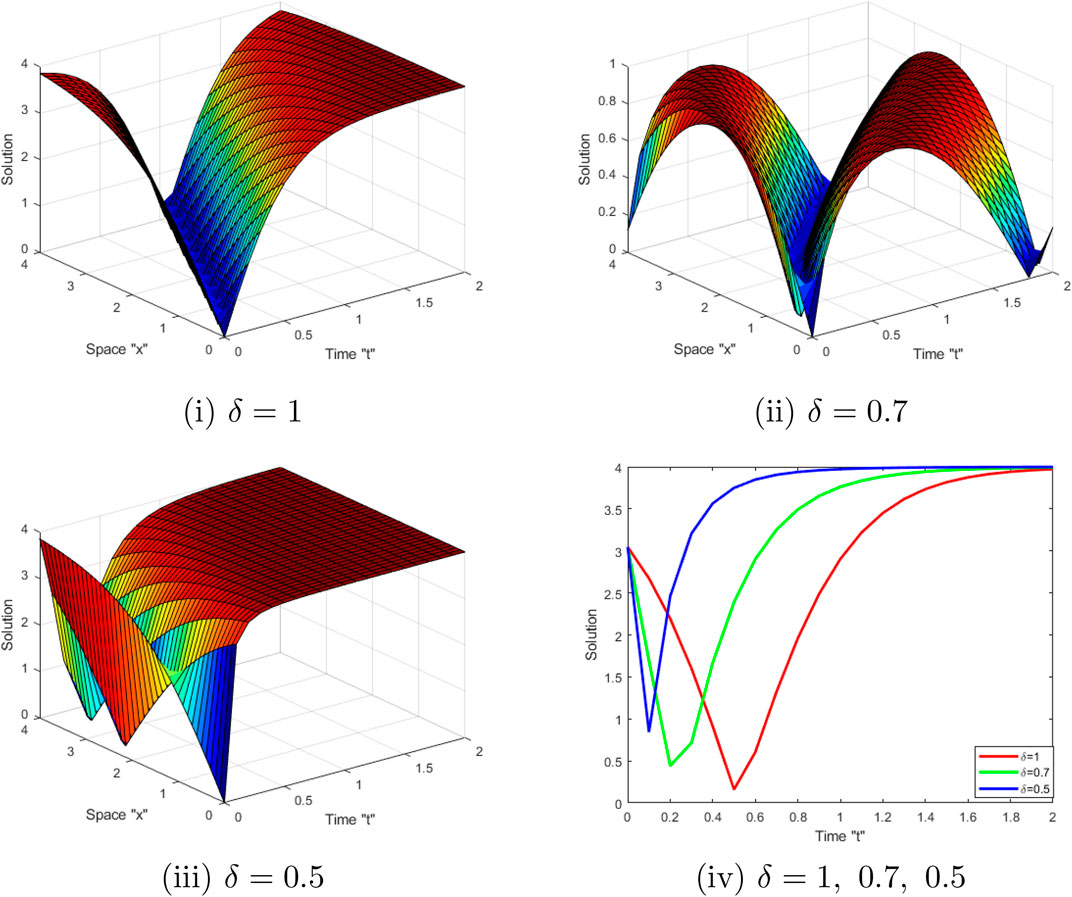
FIGURE 1. (i–iii) display 3D-shape of solution
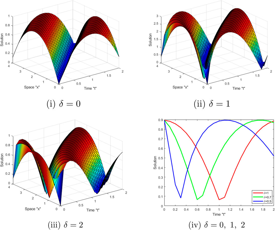
FIGURE 2. (i–iii) display 3D-shape of solution

FIGURE 3. (i–iii) display 3D-shape of solution
In this study, the Sasa-Satsuma equation with M-truncated derivative (SSE-MTD) was examined. We acquired the exact solutions by utilizing Jacobi elliptic function and generalizing Riccati equation mapping methods. Because of the application of the Sasa–Satsuma equation in explaining the propagation of femtosecond pulses in optical fibers, these solutions may explain a wide range of interesting and complex physical phenomena. Furthermore, using the MATLAB program, the M-truncated derivative effects on the exact solutions of SSE-MTD (1) were illustrated. We concluded that when the derivatives order increases the surface moves into the right. In the future work, we can consider Sasa-Satsuma equation with stochastic term.
The original contributions presented in the study are included in the article/Supplementary Material, further inquiries can be directed to the corresponding author.
WM: software, data curation, formal analysis, investigation, methodology, writing—original draft. FA-A: data curation, investigation, formal analysis, writing—original draft. All authors contributed to the article and approved the submitted version.
Princess Nourah bint Abdulrahman University Researcher Supporting Project number (PNURSP2023R 273), Princess Nourah bint Abdulrahman University, Riyadh, Saudi Arabia.
The authors declare that the research was conducted in the absence of any commercial or financial relationships that could be construed as a potential conflict of interest.
All claims expressed in this article are solely those of the authors and do not necessarily represent those of their affiliated organizations, or those of the publisher, the editors and the reviewers. Any product that may be evaluated in this article, or claim that may be made by its manufacturer, is not guaranteed or endorsed by the publisher.
2D, Two dimension; 3D, Three dimension; FNLDEs, Fractional nonlinear differential equations; GREM-method, generalizing Riccati equation mapping method; JEF-method, Jacobi elliptic function method; MTD, M-truncated derivative; ODE, Ordinary differential equation; SSE, Sasa-Satsuma equation; SW, Solitary waves.
1. Lyu W, Wang Z. Global classical solutions for a class of reaction-diffusion system with density-suppressed motility. Electron Res Archive (2022) 30(3):995–1015. doi:10.3934/era.2022052
2. Xie X, Wang T, Zhang W. Existence of solutions for the (p,q)-Laplacian equation with nonlocal Choquard reaction. Appl Math Lett (2023) 135:108418. doi:10.1016/j.aml.2022.108418
3. Zhang J, Xie J, Shi W, Huo Y, Ren Z, He D. Resonance and bifurcation of fractional quintic Mathieu–Duffing system. Chaos: Interdiscip J Nonlinear Sci (2023) 33(2):023131. doi:10.1063/5.0138864
4. Alshammari M, Iqbal N, Botmart T. The solution of fractional-order system of KdV equations with exponential-decay kernel. Results Phys (2022) 38:105615. doi:10.1016/j.rinp.2022.105615
5. Hussain S, Madi EN, Iqbal N, Botmart T, Karaca Y, Mohammed WW. Fractional dynamics of vector-borne infection with sexual transmission rate and vaccination. Mathematics (2021) 9(23):3118. doi:10.3390/math9233118
6. Alshammari M, Mohammed WW, Yar M. Novel Analysis of fuzzy fractional Klein-Gordon model via Semianalytical method. J Funct Spaces (2022) 2022:1–9. doi:10.1155/2022/4020269
7. Qt Ain QT, Anjum N, Din A, ZebDjilali AS, Khan ZA. On the analysis of Caputo fractional order dynamics of Middle East Lungs Coronavirus (MERS-CoV) model. Alex Eng J (2022) 61(7):5123–31. doi:10.1016/j.aej.2021.10.016
8. Akbulut A, Kaplan M, Tascan F. Conservation laws and exact solutions of Phi-four (Phi-4) equation via the (G′/G, 1/G) -expansion method. Z für Naturforschung A (2016) 71(5):439–46. doi:10.1515/zna-2016-0010
9. Wang ML, Li XZ, Zhang JL. The (G′/G)-expansion method and travelling wave solutions of nonlinear evolution equations in mathematical physics. Phys Lett A (2008) 372:417–23. doi:10.1016/j.physleta.2007.07.051
10. Zhang H. New application of the (G′/G)-expansion method. Commun Nonlinear Sci Numer Simul (2009) 14:3220–5. doi:10.1016/j.cnsns.2009.01.006
11. Naher H, Abdullah FA. New approach of (G′/G) -expansion method and new approach of generalized (G′/G) -expansion method for nonlinear evolution equation. AIP Adv (2013) 3(3):032116. doi:10.1063/1.4794947
12. He JH, Wu XH. Exp-function method for nonlinear wave equations. Chaos Solitons Fractals (2006) 30(3):700–8. doi:10.1016/j.chaos.2006.03.020
13. Yan ZL. Abundant families of Jacobi elliptic function solutions of the (2+1)-dimensional integrable Davey–Stewartson-type equation via a new method. Chaos Solitons Fractals (2003) 18:299–309. doi:10.1016/s0960-0779(02)00653-7
14. Wazwaz AM. The sine-cosine method for obtaining solutions with compact and noncompact structures. Appl Math a Comput (2004) 159(2):559–76. doi:10.1016/j.amc.2003.08.136
15. Jiong S. Auxiliary equation method for solving nonlinear partial differential equations. Phys Lett A (2003) 309:387–96. doi:10.1016/S0375-9601(03)00196-8
16. Lu B. The first integral method for some time fractional differential equations. J Math Anal Appl (2012) 395(2):684–93. doi:10.1016/j.jmaa.2012.05.066
17. Baskonus HM, Bulut H, Sulaiman TA. New complex hyperbolic structures to the lonngren-wave equation by using sine-gordon expansion method. Appl Math Nonlinear Sci (2019) 4(1):129–38. doi:10.2478/amns.2019.1.00013
18. Arnous AH, Mirzazadeh M. Application of the generalized Kudryashov method to the Eckhaus equation. Nonlinear Anal Modell Control (2016) 21(5):577–86. doi:10.15388/na.2016.5.1
19. Khan K, Akbar MA. The exp(−ϕ(ς))-expansion method for finding travelling wave solutions of Vakhnenko-Parkes equation. Int J Dyn Syst Differ Equ (2014) 5:72–83. doi:10.1504/ijdsde.2014.067119
20. Tao H, Anjum N, Yang Y-J. The Aboodh transformation-based homotopy perturbation method: New hope for fractional calculus. Front Phys (2023) 11:1168795. doi:10.3389/fphy.2023.1168795
21. Anjum N, He C-H, He J-H. Two-scale fractal theory for the population dynamics. Fractals (2021) 29:2150182. doi:10.1142/S0218348X21501826
22. Anjum N, Ain QT, Li XX. Two-scale mathematical model for tsunami wave. Int J Geomath (2021) 12:10. doi:10.1007/s13137-021-00177-z
23. Katugampola UN. New approach to a generalized fractional integral. Appl Math Comput (2011) 218(3):860–5. doi:10.1016/j.amc.2011.03.062
24. Katugampola UN. New approach to generalized fractional derivatives. Bull Math Anal Appl B (2014) 6(4):1–15.
25. Kilbas AA, Srivastava HM, Trujillo JJ. Theory and applications of fractional differential equations. Amsterdam, Netherlands: Elsevier (2016).
26. Samko SG, Kilbas AA, Marichev OI. Fractional integrals and derivatives, theory and applications. Yverdon, Switzerland: Gordon and Breach (1993).
27. Sousa JV, de Oliveira EC. A new truncated M fractional derivative type unifying some fractional derivative types with classical properties. Int J Anal Appl (2018) 16(1):83–96. doi:10.28924/2291-8639-16-2018-83
28. Al-Askar FM, Cesarano C, Mohammed WW. Abundant solitary wave solutions for the boiti–leon–manna–pempinelli equation with M-truncated derivative. Axioms (2023) 12(5):466. doi:10.3390/axioms12050466
29. Mohammed WW, Cesarano C, Al-Askar FM. Solutions to the (4+1)-dimensional time-fractional fokas equation with M-truncated derivative. Mathematics (2023) 11(1):194. doi:10.3390/math11010194
30. Yusuf A, Inc M, Baleanu D. Optical solitons with M-truncated and beta derivatives in nonlinear optics. Front Phys (2019) 7:126. doi:10.3389/fphy.2019.00126
31. Ozkan A, Ozkan EM, Yildirim O. On exact solutions of some space–time fractional differential equations with M-truncated derivative. Fractal and Fractional (2023) 7(3):255. doi:10.3390/fractalfract7030255
32. Bogning JR, Tchaho CT, Kafne TC. Solitary wave solutions of the modified sasa-satsuma nonlinear partial differential equation. Am J Comput Math (2013) 3:131–7. doi:10.5923/j.ajcam.20130302.11
33. Yildirim Y. Optical solitons to sasa-satsuma model in birefringent fibers with trial equation approach. Optik (2019) 185:269–74. doi:10.1016/j.ijleo.2019.03.016
34. Sasa N, Satsuma J. New-type of soliton solutions for a higher-order nonlinear Schrödinger equation. J Phys Soc Jpn (1991) 60:409–17. doi:10.1143/jpsj.60.409
35. Mihalache D, Truta N, Crasovan LC. Painlevé analysis and bright solitary waves of the higher-order nonlinear Schrödinger equation containing third-order dispersion and self-steepening term. Phys Rev E (1997) 56(1):1064–70. doi:10.1103/physreve.56.1064
36. Solli D, Ropers C, Koonath P, Jalali B. Optical rogue waves. Nature (2007) 450(7172):1054–7. doi:10.1038/nature06402
37. Khater MM, Seadawy AR, Lu D. Dispersive optical soliton solutions for higher order nonlinear Sasa-Satsuma equation in mono mode fibers via new auxiliary equation method. Superlatt Microstruct (2018) 113:346–58. doi:10.1016/j.spmi.2017.11.011
38. Chen S. Twisted rogue-wave pairs in the Sasa-Satsuma equation. Phys Rev E (2013) 88(2):023202. doi:10.1103/physreve.88.023202
39. Tuluce DS, Pandir Y, Bulut H. New soliton solutions for Sasa–Satsuma equation. Waves Random Complex Medium (2015) 25(3):417–28. doi:10.1080/17455030.2015.1042945
40. Seadawy AR, Nasreen N, Dian-chen LU. Optical soliton and elliptic functions solutions of Sasa-satsuma dynamical equation and its applications. Appl Math J Chin Univ. (2021) 36(2):229–42. doi:10.1007/s11766-021-3844-0
41. Xu T, Wang D, Li M, Liang H. Soliton and breather solutions of the Sasa–Satsuma equation via the Darboux transformation. Phys Scr (2014) 7:075207. doi:10.1088/0031-8949/89/7/075207
42. Xu J, Fan E. The unified transform method for the Sasa–Satsuma equation on the half-line. Proc R Soc A (2013) 469(2159):20130068. doi:10.1098/rspa.2013.0068
43. Liu Y, Gao YT, Xu T, Lü X, Sun ZY, Meng XH, et al. Soliton solution, bäcklund transformation, and conservation laws for the Sasa-Satsuma equation in the optical fiber communications. Z Nat A (2010) 65(4):291–300. doi:10.1515/zna-2010-0405
44. Wright OC. Sasa-Satsuma equation, unstable plane waves and heteroclinic connections. Chaos Soliton Fract (2007) 33(2):374–87. doi:10.1016/j.chaos.2006.09.034
45. Zhu SD. The generalizing Riccati equation mapping method in non-linear evolution equation: Application to (2+1)-dimensional boiti–leon–pempinelle equation. Chaos, Solitons Fractals (2008) 37:1335–42. doi:10.1016/j.chaos.2006.10.015
46. Fan E, Zhang J. Applications of the Jacobi elliptic function method to special-type nonlinear equations. Phys Lett A (2002) 305:383–92. doi:10.1016/s0375-9601(02)01516-5
47. Scott AC. Encyclopedia of nonlinear science. New York, NY: Routledge, Taylor and Francis Group (2005).
48. Rosenau P, Hyman JM, Staley M. Multidimensional compactons. Phys Rev Lett (2007) 98:024101. doi:10.1103/PhysRevLett.98.024101
49. Camassa R, Holm DD. An integrable shallow water equation with peaked solitons. Phys Rev Lett (1993) 71:1661–4. doi:10.1103/PhysRevLett.71.1661
Keywords: Sasa-Satsuma equation, M-truncated derivative, optical solitons, generalizing Riccati equation mapping method, analytical solutions
Citation: Al-Askar FM and Mohammed WW (2023) Abundant optical solutions for the Sasa-Satsuma equation with M-truncated derivative. Front. Phys. 11:1216451. doi: 10.3389/fphy.2023.1216451
Received: 03 May 2023; Accepted: 10 July 2023;
Published: 21 July 2023.
Edited by:
Hamid M. Sedighi, Shahid Chamran University of Ahvaz, IranReviewed by:
Muhammad Nadeem, Qujing Normal University, ChinaCopyright © 2023 Al-Askar and Mohammed. This is an open-access article distributed under the terms of the Creative Commons Attribution License (CC BY). The use, distribution or reproduction in other forums is permitted, provided the original author(s) and the copyright owner(s) are credited and that the original publication in this journal is cited, in accordance with accepted academic practice. No use, distribution or reproduction is permitted which does not comply with these terms.
*Correspondence: Wael W. Mohammed, d2FlbC5tb2hhbW1lZEBtYW5zLmVkdS5lZw==
†ORCID: Farah M. Al-Askar, orcid.org/0000-0002-2394-0041; Wael W. Mohammed, orcid.org/0000-0002-1402-7584
Disclaimer: All claims expressed in this article are solely those of the authors and do not necessarily represent those of their affiliated organizations, or those of the publisher, the editors and the reviewers. Any product that may be evaluated in this article or claim that may be made by its manufacturer is not guaranteed or endorsed by the publisher.
Research integrity at Frontiers
Learn more about the work of our research integrity team to safeguard the quality of each article we publish.