 Jingyu Wu1
 Lingfei Li
- 1School of Economics and Management, Northwest University, Xi’an, Shaanxi, China
- 2School of Professional Studies, Columbia University, Manhattan, NY, United States
The option is an important derivative tool in financial market, and after decades of development, the option has emerged in various forms. This paper studies an exotic option with a proactive investment strategy. Compared with the classic option theory, we assume that the option holders continuously trade the underlying assets according to a predetermined investment strategy. Taking the European call option as an example, we first give some assumptions and define the loss function in terms of a logarithmic investment strategy. Then, the specific pricing expression of the exotic option is derived from the Black-Scholes option pricing formula. Next, numerical simulations are presented to visualize the mechanism of the exotic option in 2D and 3D forms by selecting appropriate parameters. The results indicate that the exotic option has a significant price advantage (up to 43.9% under specific parameter settings) over the classic option. Moreover, the empirical results illustrate a perfect fit between 50 ETF (issued by the Shanghai Stock Exchange) and our exotic option. The new proposed exotic option extends the Black-Scholes option theory from a no-trading condition (do not buy or sell underlying assets during the validity period) to a dynamic investment condition and has important practical significance in real life.
1 Introduction
The past 50 years have witnessed the transformation of financial derivatives. In the 1970s and 1980s, investors urgently needed new financial tools to avoid risks and to acquire more returns. Therefore, options, swaps, and forward came into being, and derivative markets have become increasingly important in finance and investment. Financial derivatives could be defined as a security whose price relies on the values of more basic variables, such as underlying asset prices and interest rates. The underlying assets usually contain stocks, bonds, interest rates, foreign exchange, etc. The option studied in this paper is a contract that gives the holder the right (not the obligation) to buy or sell stocks at a predetermined price by a specific date. Options can be classified as call options and put options. A call (put) option gives the holder the right to buy (sell) stocks at the strike price or exercise price on the expiration date. Since the right is optional, whether or not the holder will exercise it depends on whether the market conditions on the expiration date are favorable to him. According to the time of exercise, options can also be divided into European options and American options. The former can only be exercised on the expiration date, while the latter can be exercised at any time before the expiration date. Because the exercise time of American options is flexible, this paper takes European options as the research object.
The revolution in trading and pricing derivatives began in the early 1970s. In April 1973, the Chicago Board of Trade set up a new exchange, the Chicago Board of Options Exchange, and started to trade options in exchanges. In the same year, Black and Scholes of the University of Chicago successfully deduced the complete option pricing formula, known as the Black–Scholes or Black–Scholes–Merton model [1, 2]. They thought that investors could set up a riskless hedging portfolio, including the option and underlying assets, so that its rate of return in a short time must equal the risk-free return rate in an efficient market without riskless arbitrage opportunity. The pricing formula of European call options is obtained as follows:
The Black–Scholes model achieved a major breakthrough in the pricing of European options and was widely used in financial practice areas. However, practitioners using the Black–Scholes model realized that its assumptions base the model on the ideal market that is quite different from the actual market. The main issues discussed are assumptions of constant volatility and interest rate, continuity of asset price, no transaction cost, no tax, no dividend, and so on. So, scholars have tried to seek an option pricing model closer to the actual market by relaxing these assumptions. Leland (1985) considered transaction costs and proposed a modification to the Black–Scholes model [3]; Merton (1978, 1982) developed the option pricing model to the case where stocks pay known dividends and stochastic interest rates [4, 5]; Ingersoll (1976) and Scholes (1976) considered different tax rates and capital gain dividends [6, 7]; Heston (1993), Xun Li, Zhenyu Wu (1985), etc. assumed the variance of an asset price to follow the stochastic process and enriched the option pricing [8, 9]; Rich (1996), Yoshida (2003), Moawia (2022), and so on developed the option pricing formula under stochastic volatility [10–12]; Jarrow (1984), Amin (1993), Ernesto Mordecki (2002), etc. studied the option pricing problem of the increase in the underlying asset price [13–15]; Schroder (1999), Korn (2002), etc. further considered the option pricing model under the condition of unfixed dividend [16–18]. In addition, many scholars tried to establish the option pricing model by other methods, such as the binomial model [19] and Monte Carlo method [20]. Recently, Cherstvy derived the reset Geometric Brownian Motion—SGBM, which describes the stochastic process more thoroughly and completely. In addition, they calculated its mean-squared displacement (MSD) and time-averaged MSD (TAMSD), which are consistent with the computer simulation results. For SGBM, compared with the classic GBM, the MSD increases faster in time than the exponential growth in the real stock market, and the TAMSD is always linear in a short lag time [21]. Importantly, by calculating the ratio between the MSD and TAMSD, an obvious inequality was found between them, which further proves that SGBM is non-ergodic [22]. Moreover, with the increasing impact of Big Data, AI, and other technological means on the financial market, machine learning algorithms have been applied to asset pricing in recent years [23–25]. So far, there are many pricing formulas, each with advantages and disadvantages. At the same time, various exotic options have also emerged. The exotic option is the option with less standardized contract terms and attributes, which is different from the traditional vanilla option in terms of payment structure, expiration date, exercise price, etc. [26]. The exotic option mainly includes barrier option, Asian option, and lookback option. These exotic options are flexible and diverse, starting from customer needs, providing investors with more investment choices [27].
Only a few works introduced additional investment strategies to option pricing. The classic Black–Scholes pricing formula implies that the option holder does not trade underlying assets before or after the expiration date and only depends on the option to avoid risk. Regardless, in the actual market, investors usually depend on various portfolios to avoid risks rather than being limited to a specific asset. Therefore, they would take the initiative to adjust their positions when the price of the underlying asset changes. From this point, Wang et al. deduced a new option pricing formula under a linear post-active investment strategy [28]. Here, “post-active” means buying or selling an underlying asset after it reaches the exercise price. In this model, when the stock price reaches a certain value, the option holder starts to trade the stock according to a pre-designed strategy. More precisely, the option holder would buy in stock as the stock price is higher than the exercise price for the call option, or sell out stock as the stock price is lower than the exercise price for the put option. Qiao et al. further proposed a non-linear post-active investment strategy [29]. Based on the aforementioned discussions, the previous works mainly focused on improving traditional option theory via a post-active strategy. Here, we are struck by an interesting idea.
1) Is it appropriate to assume the investor must act after exercising the option?
2) Are there alternative explanations for such behaviors?
3) Can we assume that investors would take action before exercising the option?
Motivated by the aforementioned questions, we introduce a proactive investment strategy that can be seen as a complement to [29]. Compared with the classic option theory, we first assume that the option holders act ahead of exercising the option since a wise investor usually has a good sense of the market and acts before the others. Second, we assume that the option holders continuously trade the underlying assets according to a non-linear investment strategy. This paper is arranged as follows: In Section 2, we put forward some basic assumptions along with a proactive non-linear position strategy and calculate the corresponding loss function. In Section 3, we give a conclusive theorem to define the analytic solution of the Black–Scholes partial differential equation, see Theorem 1. Then, the pricing formula of the new proposed option is derived based on Theorem 1. In Section 4 and Section 5, numerical simulations are presented to visualize the mechanism of the exotic option in 2D and 3D forms by selecting appropriate parameters and different investment strategies. In Section 6, we selected Shanghai 50 ETF options as the research object and further analyzed and compared the actual option price, the classic option price, and the exotic option price with a proactive investment strategy. Section 7 summarizes the paper.
2 Exotic option with a proactive investment strategy
2.1 Assumptions for the option
The construction of European call option pricing formula with a proactive investment strategy is based on the following assumptions.
1) The total amount of capital initially available to the option holder is M = Q × Xe, where Q is the number of stocks agreed in the contract and Xe is the exercise price of each unit of stocks.
2) The investors have a good judgment of the market and act before exercising the option.
3) The option holders adjust their holdings by buying or selling stocks according to a logarithmic trading strategy.
4) The stock price observes geometric Brownian motion (GBM).
5) The stock does not pay dividends.
6) The risk-free rate of interest is constant.
7) There is no transaction cost for buying and selling stocks or options.
2.2 Establishment of the proactive investment strategy
In the classic option pricing model, one can use the call option to avoid the risk caused by a rise in share price or the put option to avoid the risk caused by a drop in share price. Nevertheless, the underlying assumption is that there is no transaction (no buying or selling underlying assets) during the validity period. However, the investor is still able to buy or sell the underlying asset after purchasing the option.
Under the aforementioned assumptions, we first name δ (δ ≥ 0) as investment sensitivity. The greater its value, the earlier the investor acts. For example, when taking a short position in a bear market, wise investors cannot merely depend on the option to avoid the risk that the market will reverse. On the contrary, they will take the initiative to buy the stocks. From this point of view, the parameter δ indicates how early they take the actions in the bull market before exercising the option. Moreover, S is the stock price; Xe is the exercise price for the call option; α (α ≥ 0) is the investment strategy index, used to represent an interval that investors would act (buy the stocks) during such a period; βmax, βmin (0 ≤ βmax, βmin ≤ 1) is the maximum or minimum capital utilization rate for the initial capital M. β[S] is a general logarithmic position strategy, which is used to describe the capital utilization rate with respect to the stock price. The specific form of β[S] is written as follows:
Before the price reaches Xe − δ, the investor takes no action. When the price reaches Xe − δ, the investor begins to take action, and initially, spending βmin × M to buy in stocks that correspond to Assumption Eq. 2). The investor will not stop buy-in of the stock until the price reaches (1 + α)(Xe − δ), and the total capital of the investment is βmax × M, see Figure 1. On the contrary, if the price decreases from (1 + α)(Xe − δ) to Xe, the investor should sell the stock based on Eq. 2).
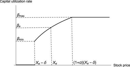
FIGURE 1. Logarithmic investment strategy.
2.3 Definition of the loss function
For the no-trading cases (classic option theory), when the stock price increases to S0 (S0 > Xe), the expected loss for each option contract is
where β′[S] is the derivative of β[S], i.e.,
Substituting in (Eq. 3), one has
Therefore, the expected loss L [S0] should be modified to
The per share loss is
Next, we will compare the intrinsic value between the exotic option and the classic option. For the exotic option, its intrinsic value is exactly per share loss obtained aforementioned, i.e.,
where
In the classic European call option defined by the Black–Scholes option pricing model, f[S] is the price of the derivative. When t = T (T is expiration date), f(S, T) is the intrinsic value function, i.e.,
To compare these two values, the parameters are set to be α = 0.8, βmin = 0.2, βmax = 0.8, Xe = 30, δ = 5. The intrinsic values of new and classic options are shown in Figure 2. It can be found that the intrinsic value of new options is equal to that of the classic one when the stock price is lower than the exercise price. As the price increases, the intrinsic value of the new option is lower than that of the traditional option. Moreover, the gap between the options increases gradually as the stock price increases continuously.
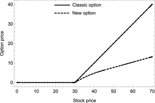
FIGURE 2. Intrinsic values of new and classic options.
3 Exotic option pricing formula of Brownian motion
3.1 Asset price behavior of Brownian motion
We recall the fractional Brownian motion with Hurst parameter H (Gaussian process WH [t], 0 < H < 1), where
for all
where μ is the expected return rate and σ is volatility. Using the Wick calculus [31], the following solution is provided
For two different times t1, t2 under the risk-free condition μ = r, one has
3.2 European call option pricing formula based on Brownian motion
In 1973, Black and Scholes pointed out that it is impossible to make profits (risk-neutral) by creating portfolios of long and short positions in options and underlying assets if options are correctly priced, and thus presented a theoretical valuation formula of options, Black–Scholes partial differential equation, i.e.,
where f is the price of the derivative, t is time, r is the risk-free interest rate, σ is the volatility of stock price, and S is the stock price.
Lemma 1. Let f be a function, and assuming that E[f[W[T]]] < ∞, then, for each t < T, one has
Proof.
Thus, f has the form
Substituting WH [T] into it, we have
along with
where I denotes inverse Fourier transformation between
it follows the fact that
where H = 1/2.
Theorem 1. [32] The analytic solution of the Black–Scholes partial differential Eq. (11) has the form
where T is the mature date and f[⋅] is the intrinsic value.
Proof. For the Black–Scholes partial differential equation
The Feynman–Kac formula indicates that its solution can be written as a conditional expectation
Then, substituting (Eq. 10) into (Eq. 14), and applying Lemma 1, one has
Setting
3.3 Pricing formula of the exotic option based on Brownian motion
We have previously discussed the solution’s mechanism of the Black–Scholes partial differential equation under Brownian motion. Next, we will derive the pricing formula of the exotic option in terms of Theorem 1. To obtain the pricing formula of the new option, one has to replace f [⋅] with Eq. 8) in Theorem 1. In this sense, the pricing formula should have three parts
where
If
If
For simplicity, we write them as
Since VT1 = 0, we start from VT2. Therefore, we have
that can be further expressed as
where
Thus, one has
where
Similarly, VT3 has the form
that can be written as
where
therefore, we have
where
Last, substituting V1, V2, V3 into (Eq. 15), the pricing formula of the exotic option can be expressed as
Next, we will discuss two special cases of (Eq. 16). The first case is βmin = βmax = 0, δ = 0, which means the investor does not take any action before or after exercising the option. By this means, the new option equals the classic option. To be specific, the parameters turn to H = 0, A = S, I = −Xe, G = −Xe, Q = 1, and (16) translates to
where
On the other hand, if we set βmin = βmax = 1, δ = 0 and α to be a sufficiently small positive constant, the option holders will spend all their capital to buy stocks as soon as the price reaches Xe, which means this action will completely cover the risk of the underlying asset. To be specific, the parameters turn to H = 0, A = 0, I = 0, G = 0, Q = 0, d1 = d2, d3 = d4 and (Eq. 16) equals 0.
Compared with the Black–Scholes option pricing formula, the new option formula has a significant price advantage. The Black–Scholes option theory is obtained under the no-trading condition (do not buy or sell underlying assets during the holding period), while the formula proposed in this paper assumes that the holder will continuously trade the underlying assets during the holding period. Specifically, when the stock price reaches the set buying point, investors begin to buy the stock according to the pre-designed non-linear strategy. When the price increases, the profits earned by investors can compensate for the losses incurred during the holding period, resulting in a total loss lower than that of classic options. Therefore, the value of exotic options is lower than that of classic options, allowing investors to obtain options at a lower price.
Importantly, we can also improve this formula by relaxing other assumptions of the Black–Scholes model. For example, we can start with the transaction costs that investors are more concerned about. In the real capital market, option trading is accompanied by a considerable amount of transaction costs that cannot be ignored. Many scholars have proposed various methods to address this issue, such as Leland. Leland divided the entire holding period into countless small time intervals, dispersing transaction costs into time intervals so that the corresponding transaction costs are proportional to the value of the underlying asset [3]. In other words, the cost is represented by κ|ξ|S, where ξ is the amount of the underlying asset sold at the stock price S and κ is the proportionality coefficient related to the investor’s preference. We can also adopt this idea to improve the formula and obtain the differential equation with transaction costs. In addition, the volatility of the underlying asset price is also a hot topic for scholars to study. In most articles, volatility is considered to be a constant in order to simplify the model and improve its computability. However, a large number of actual data show that implied volatility varies with changes in execution price and expiration time [32]. Therefore, we can improve the model by assuming that volatility is also a stochastic process and non-constant, that is, the volatility should follow the stochastic process: dσ2 = μσ2dt + νσ2dz, where μ and ν depend on σ and t, but not on S, and Wiener processes dz and dw have a correlation ρ. Similarly, we can also consider further modifications to the formula in situations such as stock dividends and taxes. These can make the pricing formula better describe market behavior and increase the difficulty of pricing, which requires further research in the future.
4 Sensitivity analysis of exotic and classic option
In this section, we will systematically analyze the mechanism of each parameter contained in the exotic option (Eq. 16). Briefly speaking, we intend to investigate what will happen to the exotic option if one of the parameters changes while the others remain fixed. Based on the aforementioned discussions, there are two types of factors influencing the option price. One is the basic parameters: 1) exercise price Xe, 2) current stock price S, 3) time to expiration T, 4) risk-free rate of interest r, and 5) volatility of stock price σ; the second type is investment strategy parameters: 6) initial capital utilization rate βmin, 7) highest capital utilization rate βmax, 8) investment strategy index α, and 9) investment sensitivity δ. The determination of initial parameter values is crucial for numerical simulation. Improper selection of parameter values can make the results deviate from reality, and they are not conducive to draw correct conclusions. So, before sensitivity analysis, the important question we need to address is how to choose parameter values.
For some basic parameters, such as the underlying asset price S, exercise price Xe, and time to expiration T, their values do not affect the analysis results, but it should be noted that only when the exercise price is less than or equal to the price of the underlying asset, the option is valuable. For volatility, regardless of the type of asset, its price volatility is generally between 0.15 and 0.5. The value of the risk-free rate of interest depends on the length of the holding period. In China, Shibor (Shanghai Interbank Offered Rate) is generally used to measure the risk-free rate of interest. The longer the holding period, the higher the risk-free rate of interest. For example, this paper assumes that the duration of the option holding period is 6 months, and the corresponding risk-free rate of interest is the arithmetic mean value of Shibor with a validity period of 6 months, which is 2.5% according to the query on China Money Online. Compared to basic parameters, what is more important is how to determine the value of parameters related to the investment strategy. We draw a large number of two-dimensional graphs to examine the impact of different values of a certain parameter on the sensitivity of other single parameters, in order to determine the initial value of the parameter. Due to space limitations and the removal of some graphics with no significant changes, only four sectional plots are shown here.
First, we drew the sectional plot in investment sensitivity and the exotic option price under two scenarios: α < 1 and α > 1, as shown in Figure 3. Obviously, no matter what value α takes, there will always be extreme points on the curve. Before the extreme point, the exotic option price decreases with increasing investment sensitivity, and after the extreme point, the option price shows exponential growth. Moreover, the larger the investment strategy coefficient, the earlier the extreme point appears. The reason for this is that the range of stock price fluctuations is limited within a certain period of time, and the investment strategy index gives investors the range to take action. If the value is too high, the price of the underlying asset cannot arrive at this standard, and if the value is too small, it limits the trading behavior of investors. Considering the low possibility of the stock price doubling within 6 months, the value of the investment strategy index should be less than 1, and the value of investment sensitivity should be less than 20. Subsequently, as shown in Figure 4, this paper examines the relationship between the exotic option price and the exercise prices when δ = 5 and δ = 10. It can be seen that regardless of the value of investment sensitivity δ, the price of the exotic option always changes in the opposite direction to the exercise price. It is worth noting that when the investment sensitivity δ = 10 and the strike price Xe is less than 15, the so-called “un-physical” structure appears, that is, some images display extremely high or low amplitudes at few points, which is also known as the singularity. In Figure 4, the un-physical structure is represented as the infinite option price. Similarly, in Figures 5, 6, un-physical structures also appear. Specifically, in Figure 5, we plotted the curves between the exotic option price and the investment strategy index when βmax = 0.5, 0.8. It can be seen that both curves have a turning point when the investment strategy index α = 0.2. Moreover, when the investment strategy index approaches 0, the price of the exotic option approaches infinity. Therefore, the value range of the investment strategy index is [0.2, 1]. As shown in Figure 6, when the investment sensitivity is δ > 13.3, the price of exotic options shows exponential growth. So, the range of investment sensitivity values is [0, 13.3]. As for the highest and initial capital utilization rates, it can be seen from Figures 5, 6 that their values do not affect the trend of the curve, but only change the range of the option price. However, it should also be noted that the initial capital utilization rate must be less than the highest capital utilization rate, i.e., βmin < βmax. In short, the range of values for each parameter of the investment strategy is 0.2 ≤ α ≤ 1, 0 ≤ δ ≤ 13.3, 0 ≤ βmin ≤ βmax ≤ 1.
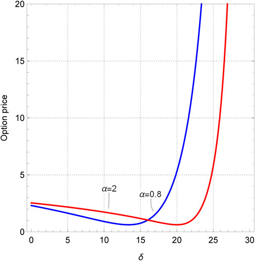
FIGURE 3. Sectional plot when α =0.5 or 1.
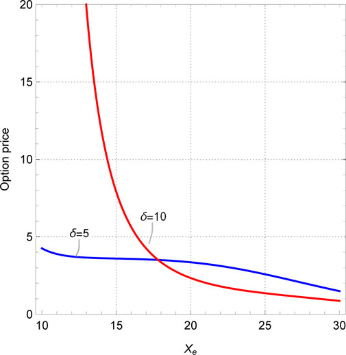
FIGURE 4. Sectional plot when δ =5 or 10.
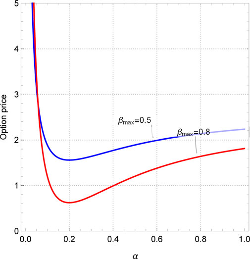
FIGURE 5. Sectional plot when βmax =0.5 or 0.8.
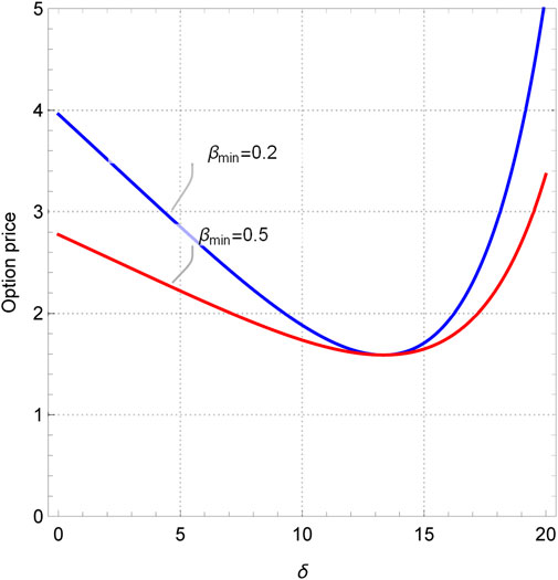
FIGURE 6. Sectional plot when βmin =0.2 or 0.5.
After clarifying the range of parameter values, we will conduct numerical simulations of option prices under different investment strategy parameters in the next section to verify the effectiveness of the proactive investment strategy.
5 Comparison of exotic and classic option under different investment strategies
Previously, we studied the mechanism of each parameter contained in the exotic option (Eq. 16). In this section, we focus on the difference between the exotic and the classic option under different investment strategies. Briefly speaking, we select several different values of α, βmin, βmax, δ to analyze and compare the price difference between the option price calculated by the Black–Scholes option pricing formula and the new option pricing formula when t = 0, Xe = 30, S = 30, T = 0.5, r = 0.025 (see Table 1).
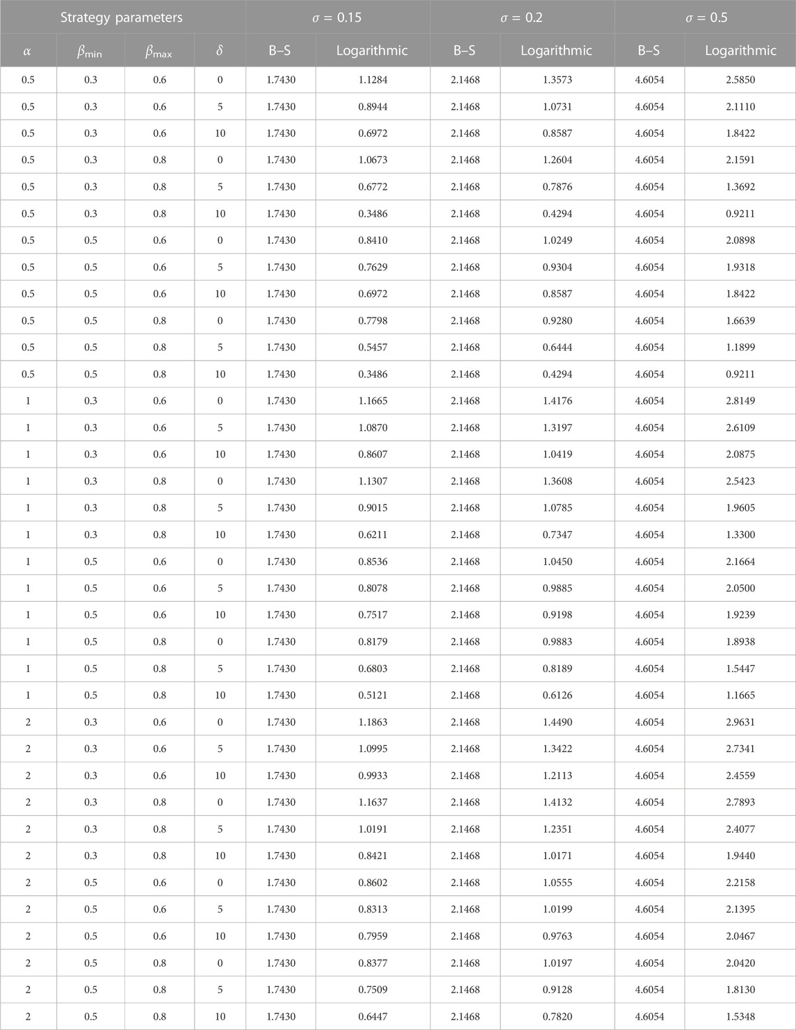
TABLE 1. Option prices under different investment strategies.
The results in Table 1 indicate:
1) Regardless of the value of the parameter, the theoretical price of the option under the logarithmic investment strategy is lower than that of the classic option. This result means that actively trading stocks can effectively reduce risks and losses, thus reducing the value of options. In this way, the European call option with the logarithmic investment strategy would likely be more attractive to investors in the financial market.
2) The price difference between the new and classic options is not invariant but varies with the change of investment strategy. For example, when the other variables are the same, the smaller the value of α(α ≥ 0), or the larger the values of βmin, βmax (0 ≤ βmin ≤ βmax ≤ 1) and δ(δ ≥ 0), the lower the price of the new option, and the larger the price difference. Specifically, when α = 0.5, βmin = 0.3, βmax = 0.6, δ = 0, σ = 0.15, the new option price is 1.1284; when δ = 5, the price is 0.8944, and when δ increases to 10, the price becomes 0.6972.
3) The volatility of stock price has a significant impact on the price difference between the new and classic options. From Table 1, we can see that when α = 0.5, βmin = 0.3, βmax = 0.6, δ = 0, and σ = 0.15, the new option is 64.7% of the classic option. When σ = 0.2, it becomes 63.2%, and when σ increases to 0.5, the proportion decreases to 56.1%. It is clear that the higher the volatility, the higher the value of the new option, and the smaller the price difference between the new and the classic option.
The aforementioned results show that no matter how the four investment strategy parameters vary, the new option is always lower than the classic option, which verifies the effectiveness of the policy.
Next, we will examine these effects in three-dimension plots. Specifically, we combine the parameters in pairs and draw three-dimensional pictures of the options. According to the proactive investment strategy (Eq. 2) (also see Figure 1), there are five free parameters βmax, βmin, Xe, α, δ in total, and ten pairs if we pair them. In order to save space, we only select four conditions here.
When drawing 3D plots, we found that the prices of exotic options in certain regions are inconsistent with the assumptions. First, based on our hypothesis, the option price should be greater than or at least equal to 0, but there is a situation where the option price is negative in the image. Second, the returns obtained by investors buying stocks in advance can compensate for more losses, making the total loss of the exotic option lower or equal to that of the classic option. Therefore, the price of exotic options should be lower or at least equal to that of classic options. However, in certain regions of the image, the price of the exotic option is higher than that of the classic option, which is apparently unreasonable. In addition, there are some implicit conditions, for example, the option is valuable only when the exercise price is lower than the underlying asset price, and the initial capital utilization rate is lower than the highest utilization capital rate. In summary, in order to make the graphics more reasonable, we have added the following constraints: 1) the exotic option should be less than or equal to the classic option, 2) the exotic option should be positive or at least equal to 0, 3) 0 ≤ βmin ≤ βmax ≤ 1, and 4) the underlying price should be greater than or equal to the strike price.
First, we plot the exotic option (Eq. 16) and the classic option (Eq. 17) in the (βmax, βmin)-plane, where Xe = 20, S = 20, t = 0, T = 0.5, r = 0.025, σ = 0.3, α = 0.8, δ = 5. As shown in Figure 7, the classic option demonstrates as a plain wave since Eq. 16 does not contain βmax, βmin, and the exotic option displays as an inclined plane. It is obvious that the new option is always lower (equal at only one point) than the classic option. When βmin = βmax = 0, the classic option equals the exotic option; it is 2.07. This condition means the investor does not take any action before or after exercising the option, which exactly accords with the assumption of the classic option theory. Moreover, the reader may find that the new option possesses a wired appearance and looks like a triangle. This is because of the existence of the constraint 0 ≤ βmin ≤ βmax < 1. Actually, there are also other constraints that should be considered while studying the relevance between the two options. Above all, the new option should at least be equal to the classic option or lower than the classic option. The exotic option proposed in this paper is based on a dynamic investment strategy. This strategy makes people initiatively buy or sell the underlying asset, which reduces the risk. Therefore, the new option should be lower than the classic option or at least be equal to it. The second constraint is the exotic option should be positive or at least equal to 0. It should be noted that the prices of the exotic option might be negative under some parametric selections, which means it is only valid for a small parametric range. This property has been omitted in some related works. As we have stated previously, in order to make the new option positive, one has to narrow the range of the parameter, which also narrows the range of application. On the contrary, we can solve it from the source, such as choosing an appropriate investment strategy. The third constraint is 0 ≤ βmin ≤ βmax ≤ 1. The last one is when calculating the option price through the Black–Scholes formula; the stock price should be above the exercise price. We conclude the aforementioned constraints in the following section. Second, we plot the exotic option (Eq. 16) and the classic option (Eq. 17) in the (Xe, α)-planes separately, where S = 20, t = 0, T = 0.5, r = 0.025, σ = 0.9, βmin = 0.1, βmax = 0.8, δ = 5 for Figure 8. Similar to the last case, the classic option in Figure 8 displays as a plain wave, and the exotic option displays as an inclined plane. Moreover, it only possesses one tendency with respect to α and Xe: the option value increases (decreases) as α and Xe decreases (increases). It should be noted that there were positive parts in both pictures but were removed by the constraints.
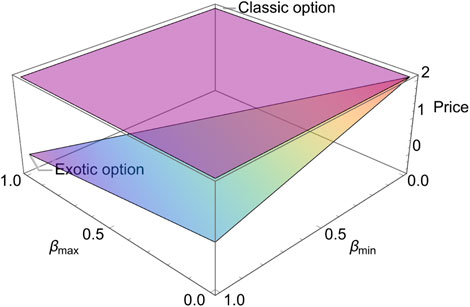
FIGURE 7. Option price in (βmax, βmin)-plane.
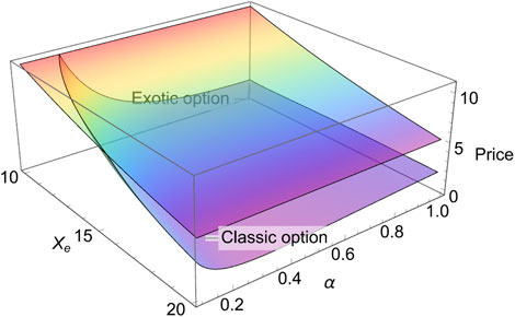
FIGURE 8. Option price in (Xe, α)-plane.
Next, we plot the exotic option (16) and the classic option (17) in the (βmax, δ)- and (βmax, α)- planes separately, where Xe = 20, S = 20, t = 0, T = 0.5, r = 0.025, σ = 0.3, α = 0.8, βmin = 0.1 for Figure 9 and Xe = 20, S = 20, t = 0, T = 0.5, r = 0.025, σ = 0.3, α = 0.8, βmin = 0.1, δ = 5 for Figure 10. As we can see in Figure 9, the classic option displays a constant wave that equals 2.07, and the exotic option is lower than the classic option. With the increase of δ, the new option gets a smaller value. Regardless, the minimum value does not locate at (1, 10). Actually, it locates at (1, 8.88). However, it looks like such a result does not comply with the assumption “the greater its value, the earlier the investor acts” in Section 2. For the dynamic investment strategy proposed, here is an elaborate non-linear function composed of logarithmic and linear functions. In particular, the variable of logarithmic function has a more complex structure, which may easily result in singularity and unexpected outcomes. Therefore, the numerical results may not be consistent with the assumptions. So, when we set to function in future research, we should fully consider the advantages and disadvantages of combining functions of different types. As shown in Figure 10, the classic option is a constant wave that equals 2.07 and the exotic option displays as a twisted wave. Actually, there is a part of the image of the exotic option above the classic option near the area α = 0. Such a part is removed by the constraint we mentioned previously. Moreover, except for the constraints applied to the exotic option, we should also pay attention to the so-called “un-physical” structure, that is, some images display extremely high or low amplitudes at a few points, which is also known as the singularity, and at these points, the exotic option deviates from reality. Therefore, in this section, we mainly discuss four examples that contrast to ten cases in total. In addition, from these four examples, we can see that the price of the exotic option with a proactive investment strategy is always lower than or equal to that of the classic option, which is the advantage of the exotic option. Adopting a proactive investment strategy can enable investors to obtain the same level of risk protection at a lower price, making them more likely to be favored by investors.
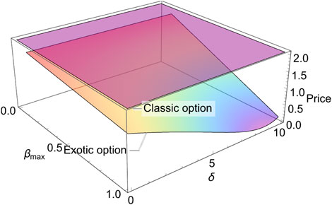
FIGURE 9. Option price in (βmax, δ)-plane.
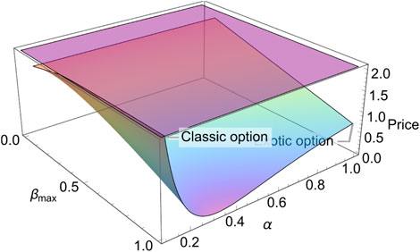
FIGURE 10. Option price in (βmax, α)-plane.
6 Empirical test
6.1 Source and description of data
In order to verify the price advantage of the new option pricing formula, we select the 50EFT option of Shanghai Stock Exchange as research object, because it is one of the most actively traded options. Specifically, the 50 ETF option contract (1004944) with an exercise price of 2.70 and expiring in February 2023 is taken as an example. The relevant parameters are obtained through the following methods.
1) The underlying asset price S: The underlying asset of this option contract is the Huaxia Shanghai Stock Exchange 50 Trading Open End Index Securities Investment Fund (code: 510050), whose price is obtained through the official website of the Shanghai Stock Exchange.
2) Exercise price Xe: The exercise price of the option contract is 2.80.
3) Time to expiration T: We assume that investors will purchase this option contract on 9 January 2023, with 45 days remaining until the expiration date of February 22.
4) Risk-free rate of interest r: The risk-free rate of interest in the Chinese capital market is usually measured in Shibor (Shanghai Interbank Offered Rate). Therefore, this paper selects the arithmetic average of 2.25% of the monthly Shibor quotation during the holding period as the risk-free rate of interest, which is sourced from the China Currency Network.
5) The volatility of the underlying asset returns σ: The volatility is based on the historical volatility of 0.1850, which is provided by the stock trading platform.
6.2 Setting investment strategy
This article assumes that investors believed that the Shanghai Stock Exchange 50 ETF price would decrease in April based on the price trend in March, so they sold all 50 ETF on 9 January 2023. At the same time, to avoid the loss caused by the rise in stock price, investors bought the call option contract expiring in April. Furthermore, based on the sensitivity analysis mentioned previously, this paper sets the highest capital utilization rate βmax = 0.8, the initial capital occupancy utilization rate βmin = 0.2, and the investment strategy index α = 0.8. The determination of investment sensitivity δ is the key to the feasibility of investment strategies, as high investment sensitivity will exceed the fluctuation range of the underlying asset price, and small investment sensitivity will bring a large number of transaction costs to investors. Therefore, this paper determines investment sensitivity according to the following formula
where T is the time to expiration; pmax,i, pmin,j is the highest and lowest prices of the underlying asset, respectively; and N is the pre-designed number of stock transactions. In this example, the highest price of the Shanghai Stock Exchange 50 ETF fund from 26 November 2022 to 9 January 2023, was 2.7250, and the lowest price was 2.5250. The pre-designed number of stock transactions is set to 2, so the investment sensitivity calculated by Eq. 18 is 0.1, that is, when the stock price reaches S1 = Xe − δ = 2.60 and S2 = Xe = 2.70, the investor uses 20% of their capital to buy the stock. In addition, when investors purchase options, they sign investment agreements with them or entrust a third party to implement strategies, stipulating that investors can only buy or sell stocks once a day.
6.3 Comparative analysis of exotic option price
According to previous assumptions, we selected the option contract data from January 9 to February 22, calculated the theoretical price of options according to the call option pricing model with a proactive investment strategy and the classic Black–Scholes call option pricing model, and compared them with the actual price to verify the effectiveness of the strategy. Meanwhile, in order to compare the impact of investment sensitivity on option prices, this paper selects different investment sensitivities. The calculation results are shown in the table as follows.
According to the data in Table 2, by comparing the theoretical price and the actual price of the option contract, it can be found that the theoretical price of the call option calculated according to the classic Black–Scholes pricing model is somewhat different from the actual price, but the maximum difference between the two is 0.0094, which is caused by the large fluctuation of the stock price on the day before the expiration date (21 February 2023). The minimum value of the difference is only 0.0002. At the same time, the option price under the proactive non-linear investment strategy is always lower than the B–S theoretical price and actual price. In addition, investment sensitivity is an important factor affecting option prices. For example, on 9 January 2023, when investment sensitivity δ = 0.05, the theoretical price of the exotic option is 0.0751; when investment sensitivity δ = 0.1, the theoretical price of the exotic option is 0.0731; and when investment sensitivity δ = 0.2, the theoretical price of the option is 0.0690. It can be seen that under the same other conditions, the theoretical price of exotic options under the proactive non-linear investment strategy shows a reverse change in investment sensitivity, that is, the higher the investment sensitivity, the lower the price of the exotic option, which is consistent with the previous analysis.
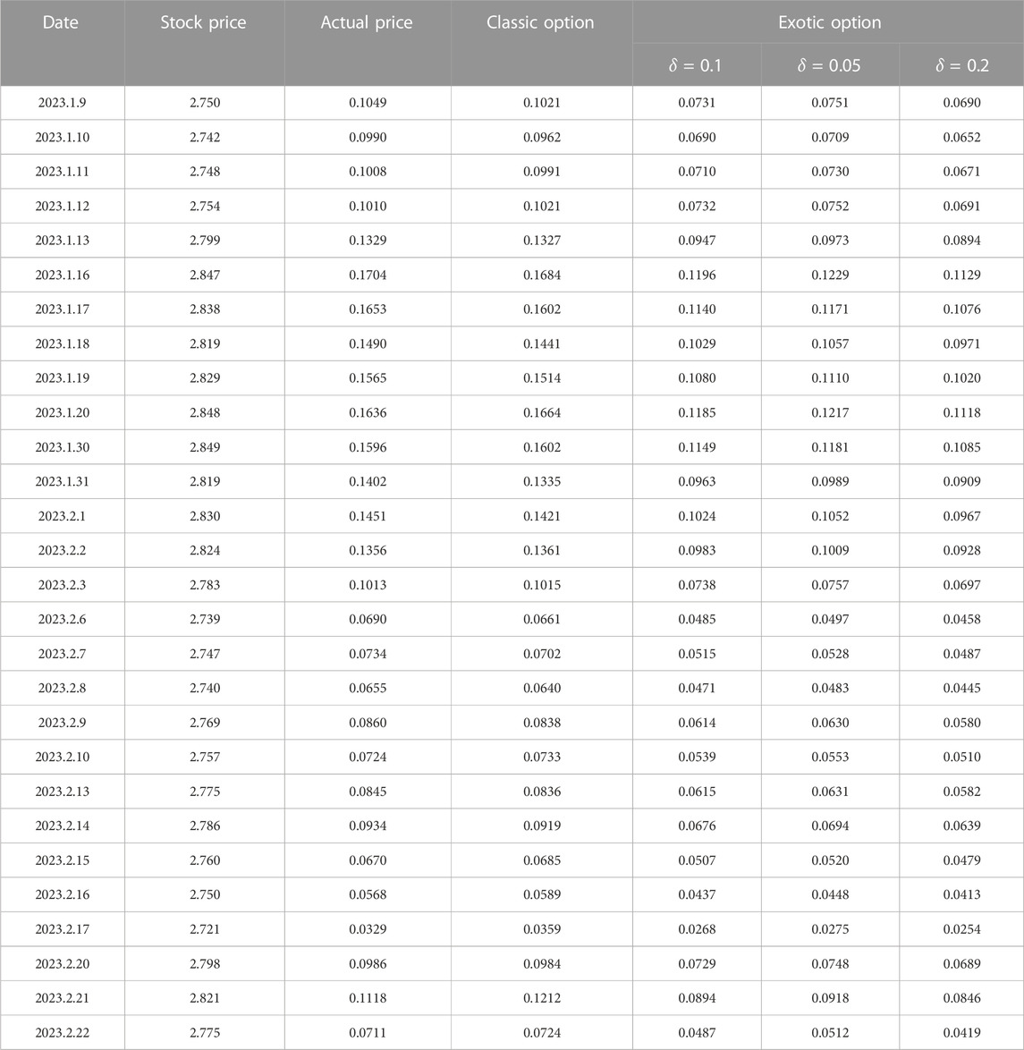
TABLE 2. Comparison of option price.
In order to compare and analyze option prices more intuitively, we have drawn the five groups of option prices into a line chart (see Figure 11). We can infer that the theoretical price of the classic option has been fluctuating around the actual price. In addition, both the actual price and the theoretical price calculated according to the Black–Scholes pricing model are higher than the exotic option price with the proactive investment strategy, which once again verifies the effectiveness of the investment strategy formulated in this paper. Furthermore, by comparing the prices of exotic options under different investment sensitivities, it can be found that exotic option prices with higher investment spacing sensitivity are lower, while exotic option prices with lower investment sensitivity are higher. According to the definition of investment sensitivity, the more sensitive investors are to market conditions, the earlier they take action, and the more losses they can compensate for, and the lower the value of options.
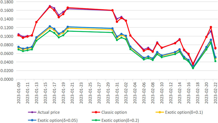
FIGURE 11. Logarithmic investment strategy.
7 Summary
This paper systematically discussed the construction of an exotic option with a proactive non-linear position strategy that presumes investors would trade the underlying asset ahead of exercising the option to avoid risk. Compared with the classic option, the newly proposed exotic option extends the Black–Scholes option theory from a static form of the no-trading case (no trading of the underlying asset during the life of the option) to a dynamic investment case, where the investor is assumed to buy or sell the underlying asset even before the option expires. According to the exotic option setting, when the stock price continues to increase and reaches the buy point (less than the strike price), the investor begins to buy and sell the stock according to a pre-designed investment strategy, and the gains from holding the stock make up for more losses, making the value of the exotic option lower than the classic option.
Except for the theoretical analysis, numerical simulations were also employed to visualize the mechanism of the exotic option in 2D and 3D forms. According to the sensitivity analysis in Section 4, investment strategy index α, investment sensitivity δ, and maximum and minimum capital utilization rates βmax, βmin all have a distinct influence on the option price. Importantly, our numerical results indicated that the exotic option has a significant price advantage over the classic option. With all other remaining parameters constant, the price of the exotic option can reach 43.9% of that of the classic option. In other words, investors can obtain the same amount of hedge as classic options at half the price of the classic option under the condition that they follow a pre-designed non-linear position strategy, which has important practical implications in real life. Furthermore, this paper takes the Shanghai Stock Exchange 50 ETF option contract in China as the research object, which compares its actual price with the theoretical price, and concludes that the price of the exotic option with a proactive investment strategy is lower than that of the classic option, which is consistent with the theoretical analysis results of this paper.
Additionally, when comparing them with different investment strategies, the parameters should observe certain constraints, meaning it is only valid for a small parametric range. On one hand, our option has a price advantage over the classic one. On the other hand, our position strategy narrows the range of applications. Just as the saying goes, “There are both advantages and disadvantages.” However, our new option was shown to be positive in most domains, while some other constructed options might be negative under certain parametric selections. The negative parts further narrow the range of applications. After all, our option still has broadened application ranges. In the future, we will make further improvements to the options and consider incorporating more features of interest to investors to expand the scope of application of the new options. Moreover, since the price of the underlying asset observes geometric Brownian motion, and the Schrödinger equation also models the random walk of particles in quantum mechanics, it is natural to use the Schrödinger equation to predict the option price. Our future work focuses on giving rigorous proof of the connection between those equations and other analytic solutions.
Data availability statement
The original contributions presented in the study are included in the article/supplementary material, further inquiries can be directed to the corresponding author.
Author contributions
JW, YW, and MZ contributed to the conception and design of the study. HZ organized the database. LL performed the statistical analysis. JW wrote the first draft of the manuscript. YW and LL wrote sections of the manuscript. All authors contributed to the article and approved the submitted version.
Conflict of interest
The authors declare that the research was conducted in the absence of any commercial or financial relationships that could be construed as a potential conflict of interest.
Publisher’s note
All claims expressed in this article are solely those of the authors and do not necessarily represent those of their affiliated organizations, or those of the publisher, the editors, and the reviewers. Any product that may be evaluated in this article, or claim that may be made by its manufacturer, is not guaranteed or endorsed by the publisher.
References
1. Black F, Scholes M. The pricing of options and corporate liabilities. J Polit Econ (1973) 81:637–54. doi:10.1086/260062
2. Merton RC. Theory of rational option pricing. Bell J Econ Manage Sci (1973) 4:141–83. doi:10.2307/3003143
3. Leland HE. Option pricing and replication with transactions costs. J Finance (1985) 40:1283–301. doi:10.1111/j.1540-6261.1985.tb02383.x
4. Merton RC, Scholes M, Gladstein M. The returns and risks of alternative put-option portfolio investment strategies. J Bus (1982) 55:1–55. doi:10.1086/296153
5. Merton RC, Scholes M, Gladstein M. The returns and risk of alternative call option portfolio investment strategies. J Bus (1978) 51:183–242. doi:10.1086/295995
6. Ingersoll JE. A theoretical and empirical investigation of the dual purpose funds: An application of contingent-claims analysis. J Financ Econ (1976) 3:83–123. doi:10.1016/0304-405x(76)90021-0
7. Scholes M, Benston GJ, Smith CW. A transactions cost approach to the theory of financial intermediation. J Finance (1976) 31:215–31. doi:10.1111/j.1540-6261.1976.tb01882.x
8. Heston S. A closed-form solution for options with stochastic volatility with applications to bond and currency options. Rev Financ Stud (1993) 6:327–43. doi:10.1093/rfs/6.2.327
9. Li X, Wu ZY. On jumps in common stock prices and their impact on call option pricing. J Finance (1985) 40:155–73. doi:10.1111/j.1540-6261.1985.tb04942.x
10. Rich D. The valuation and behavior of black-scholes options subject to intertemporal default risk. Rev Deriv Res (1996) 1:25–59. doi:10.1007/bf01536394
11. Yoshida T, Otaka M. Study on option pricing in an incomplete market with stochastic volatility based on risk premium analysis. Math Comput Model (2003) 38:1399–408. doi:10.1016/s0895-7177(03)90143-9
12. Moawia A. New developments in econophysics: Option pricing formulas. Front Phys (2022) 10:1036571.
13. Jarrow R, Rosenfeld E. Jump risks and the intertemporal capital asset pricing model. J Bus (1984) 57:337–51. doi:10.1086/296267
14. Amin KI. Jump diffusion option valuation in discrete time. J Finance (1993) 48:1833–63. doi:10.1111/j.1540-6261.1993.tb05130.x
15. Ernesto M. Optimal stopping and perpetual options for LÍęvy processes. Finance Stoch (2002) 6:473–93.
16. Schroder M. Changes of numeraire for pricing futures, forwards, and options. Rev Financ Stud (1999) 12:1143–63. doi:10.1093/rfs/12.5.1143
17. Korn O. Drift matters: An analysis of commodity derivatives. J Futures Markets (2002) 25:211–41. doi:10.1002/fut.20139
18. Whaley RE. On the valuation of American put options on dividend-paying stocks. Adv Futures Options Res (1988) 3:29–58.
19. Cox JC, Ross SA, Rubinstein M. Option pricing: A simplified approach. J Financ Econ (1979) 7:229–63. doi:10.1016/0304-405x(79)90015-1
20. Nguyen TL. Analytical approach to value options with state variables of a lévy system. Rev Financ (2003) 7:249–76. doi:10.1023/a:1024525216175
21. Cherstvy AG, Vinod D, Aghion E, Sokolov IM, Metzler R. Scaled geometric Brownian motion features sub- or superexponential ensemble-averaged, but linear time-averaged mean-squared displacements. Phys Rev E (2021) 103(6):062127. doi:10.1103/PhysRevE.103.062127
22. Vinod D, Cherstvy AG, Wang W, Metzler R, Sokolov IM. Nonergodicity of reset geometric Brownian motion. Phys Rev E (2022) 105(1):L012106. doi:10.1103/PhysRevE.105.L012106
23. Wysocki M, Slepaczuk R. Artificial neural networks performance in WIG20 index options pricing. Entropy (2022) 24:35. doi:10.3390/e24010035
24. Salvador B, Oosterlee CW, van der Meer R. Financial option valuation by unsupervised learning with artificial neural networks. Mathematics (2021) 9:46. doi:10.3390/math9010046
25. Teng YY, Li YC, Wu XB. Option volatility investment strategy: The combination of neural Network and classical volatility prediction model. Discrete Dyn Nat Soc (2022) 8952996:1–39. doi:10.1155/2022/8952996
26. Bouzoubaa M, Osseiran A. Exotic options and hybrids: A guide to structuring, pricing and trading. Wiley (2010).
28. Wang X, Wang L. Study on black-scholes option pricing model based on general linear investment strategy (part ∏: Call option). Int J Innov Comput Inf Control (2009) 5:2169–88.
29. Qiao LX, Sun FF, Qiao X, Li M, Wang X. Proactive hedging European option pricing with a general logarithmic position strategy. Discrete Dyn Nat Soc (2022) 4735656:1–18. doi:10.1155/2022/4735656
30. Hull J, White A. The pricing of options on assets with stochastic volatilities. J Finance (1987) 42(2):281–300. doi:10.1111/j.1540-6261.1987.tb02568.x
31. Hu Y, Oksendal B. Fractional white noise calculus and applications to finance. Infin Dimens Anal Qu (2003) 6:1–32. doi:10.1142/S0219025703001110
Keywords: option pricing, Black–Scholes model, dynamic investment, European call option, numerical simulation
Citation: Wu J, Wang Y, Zhu M, Zheng H and Li L (2023) Exotic option pricing model of the Black–Scholes formula: a proactive investment strategy. Front. Phys. 11:1201383. doi: 10.3389/fphy.2023.1201383
Received: 06 April 2023; Accepted: 22 May 2023;
Published: 08 June 2023.
Edited by:
Şuayip Yüzbaşi, Akdeniz University, TürkiyeReviewed by:
Sergio Da Silva, Federal University of Santa Catarina, BrazilAndrey Cherstvy, University of Potsdam, Germany
Copyright © 2023 Wu, Wang, Zhu, Zheng and Li. This is an open-access article distributed under the terms of the Creative Commons Attribution License (CC BY). The use, distribution or reproduction in other forums is permitted, provided the original author(s) and the copyright owner(s) are credited and that the original publication in this journal is cited, in accordance with accepted academic practice. No use, distribution or reproduction is permitted which does not comply with these terms.
*Correspondence: Lingfei Li, aW5mZWkyMDA2QDE2My5jb20=