A pilot study on intracerebral hemorrhage imaging based on electrical capacitance tomography

Introduction: Intracerebral hemorrhage (ICH) is a devastating disease with high rates of mortality and disability. The survival rate and postoperative outcome of ICH can be greatly improved through prompt diagnosis and treatment. CT and MRI are now the gold standards for the diagnosis of ICH, but they are not practical for use in pre-hospital emergencies or at the bedside monitoring.

Methods: Based on the earlier research of ICH detection with a single parallel plate electrode sensor, we developed a 16-electrode Electrical Capacitance Tomography (ECT) system for two-dimensional tomographic imaging of ICH in this study. A 5-layer spherical numerical model and an ex vivo porcine physical model of ICH were created for ECT simulation imaging and actual imaging, respectively, to assess the feasibility of this ECT for ICH imaging.

Results: The bleeding circles were easily seen in the image reconstruction in numerical imaging. In ex vivo imaging, the existence of bleeding was also more clearly shown with the ECT system; however, the position of the bleeding reconstructed in the image was offset by 3 mm from the real site.

Discussion: The study analyzes the causes of this discrepancy and discusses the steps that may be taken to rectify it. Overall, the simulation and ex vivo experimental trials validated the potential of ICH imaging with the ECT method; however, further work is required to increase the performance of the ECT and a more advanced imaging reconstruction algorithm is urgently needed for ICH imaging.

1 Introduction

Spontaneous intracerebral hemorrhage is caused by the rupture of blood vessels in the brain parenchyma. It is considered the most serious type of acute stroke because of its emergency, dangerous condition, high morbidity, and mortality. ICH accounts for 2.8 million fatalities annually, with the annual incidence rate of 4.1% [1]. The incidence rate of hemorrhagic stroke in China was 126.34 per 100,000 person-years [2], as reported in the 2018 China Stroke Prevention and Treatment Report. The survival rate and postoperative outcome of ICH may be greatly enhanced with early identification and treatment [3]. Currently, CT and MRI scans are the most important methods for detecting ICH; however, a significant amount of time is lost between transporting the patient to the hospital, performing the CT examination, and receiving the final result, resulting in a missed window of opportunity to treat the condition. The second is that an excessive postoperative bleeding after a hemorrhage often occurs in clinics [4]. Therefore, a portable, low-cost, and fast technology for detecting ICH is urgently needed.

Methods such as electrical impedance tomography (EIT) and magnetic induction tomography (MIT) were developed to detect ICH by measuring electrical resistivity and conductivity with a multi-sensor surrounding a head from all directions to reconstruct the resistivity and conductivity distributions in the brain over the cross section, as blood has different values for these parameters than the rest of the brain tissues [5, 6]. EIT and MIT are promising tomography technologies because of their advantages such as being non-intrusive and non-invasive. Cerebral stroke imaging with EIT and MIT methods has been researched more often and has produced some results, although there are still some issues [7–9]. Due to the relatively high electrical impedance of the skull, there is a considerable attenuation of the excitation current in EIT. Second, EIT requires the connection of electrodes with the scalp, which results in a very large contact impedance. These problems lead to low sensitivity of EIT to brain tissue imaging. As for MIT, the induced magnetic field generated in biological tissues exposed to an excitation field is negligible because of the poor conductivity of biological tissues (0.1 S/m–2 S/m) [10]. Furthermore, the conductivity of blood is not noticeably different from those of other brain tissues [11]. Because of these two factors, MIT has relatively poor sensitivity for visualizing a brain hemorrhage.

Studies of the dielectric properties of brain tissues show that the permittivity of blood is much higher than that of other tissues. At 1 MHz, the permittivity of blood, gray matter, and cerebrospinal fluid is 3,000, 990, and 108, respectively [11]. Though the permittivity of all brain tissues drops with frequency, the permittivity of blood is uniformly larger. Therefore, in theory, imaging the permittivity distribution is preferable to imaging the conductivity distribution of brain tissues for detecting cerebral hemorrhage. We have measured the change in the permittivity in the process of an ICH with a single-channel previously. First, we employed a transmitting coil and a receiving coil, based on the MIT principle, to measure the real part change in ΔB/B (the induced magnetic field ΔB is relative to the excitation field B) during ICH in a rabbit’s head, that is, to measure the change in the brain permittivity, as the information of the permittivity of the measured object is stored in the real part of ΔB/B [12], as deduced by Griffiths et al [6]. Changes in the real part of ΔB/B were found to be approximately proportional to the volume of the blood injected [12]. As the real part of ΔB/B is very small, it is extremely hard to measure and is constrained by a wide variety of factors. Next, we used a parallel-plate capacitor to directly measure the capacitance of the head during hemorrhage, with the resulting changes in capacitance reflecting the corresponding changes in hemorrhage volume [13]. The capacitance of the parallel-plate increased with increasing blood injection volume, as shown in animal experiments [13]. These two experiments suggest that it is indeed possible to reflect the amount of hemorrhage by detecting changes in the brain permittivity. Based on these results, this paper tries to use a multi-parallel-plate electrode to measure the capacitance of the brain in each projection and attempts to realize two-dimensional tomographic imaging of cerebral hemorrhage with the capacitance data and a reconstruction algorithm. This imaging method is known as ECT, which is based on capacitance measurements from a multi-electrode sensor surrounding an object (such as a pipeline or a vessel containing gas, oil, and water in the industry), and has been under development for more than a decade [14]. ECT has been widely used in multiphase flow measurements in the oil industry and fluidized bed measurements in the pharmaceutical industry [15, 16]. Apart from industrial applications, ECT is used to detect breast cancer and brain tumors and to image brain activity [17–19]. W.P. Taruno et al. used a sensor with hemispherical electrode distribution for breast cancer detection based on the fact that the permittivity of the cancerous breast cells is higher than that of healthy breast tissue [17]. They designed an actual phantom in which a paraffin wax (ε_r = 1) imitates human breasts and a rubber ball (ε_r = 80) imitates cancer cells. The phantom was used for three-dimensional ECT imaging. The results showed that the malignant cancerous cells were successfully reconstructed. ECT has also been applied for the detection of brain tumor where abnormal electrical activity around the tumor area is detected [18]. Five patients suffering from ependymoma, oligodendroglioma, craniopharyngioma, germinoma pineal, and cerebellopontine angle tumors were detected using the three-dimensional ECT system [19]. The study showed a positive correlation with MRI and CT results. We measured the change in capacitance during cerebral hemorrhage in animals using a single electrode pair and found that the amount of hemorrhage and the change in capacitance were approximately linearly correlated; this established a foundation for future studies on 2D ECT imaging of cerebral hemorrhage. This paper presents the development of a 16-electrode ECT 2D imaging system. Then, a numerical hemorrhage model and an isolated porcine brain hemorrhage model are developed to test the performance of the designed ECT system through simulation imaging and actual measurement imaging and confirm the feasibility of ECT for ICH imaging.

2 Materials and methods

2.1 Principle of ECT

A typical ECT system comprises three main units: a multi-electrode sensor, sensing electronics, and a computer for hardware control and data processing, including image reconstruction. All electrodes, usually 8 or 12, are mounted around a pipe or vessel, and the capacitance values between all single electrode combinations are measured. The sensing electronics are used to switch one electrode being connected from an excitation signal to a measurement circuit and convert the capacitance into voltage signals, which are digitized for data acquisition. The computer controls the system hardware and implements image reconstruction to show the permittivity distribution. The ECT procedure involves the forward problem and the inverse problem [20]. The forward problem is to calculate or measure the capacitance between all electrode pairs in the sensor. For a complete measurement process, one of the electrodes is selected in turn as the excitation electrode and others as detection electrodes to obtain the capacitance data between all electrode pairs. With this measurement strategy, the number of independent capacitance measurements is

$M=\frac{K\left(K-1\right)}{2}(1)$

where K is the number of electrodes. For a 16-electrode sensor, 120 independent capacitance measurements can be measured from different electrode pairs. Capacitance data are a response to the presence of permittivity distribution inside the imaging region and is calculated or measured based on the integration of Poisson’s equation (20):

$C=\frac{Q}{V}=-\frac{1}{V}{\displaystyle \int \underset{\mathrm{\Gamma }}{\int }}\epsilon \left(x,y\right)\nabla \varphi \left(x,y\right)d\mathrm{\Gamma }(2)$

where ε(x, y) is the permittivity distribution in the sensing field, V is the voltage difference between one electrode pair forming the capacitance C, $\varphi \left(x,y\right)$ is the potential distribution, and Г is the electrode surface; $\varphi \left(x,y\right)$ also depends on the permittivity distribution of ε(x, y). Therefore, the capacitance C between one electrode pair can be considered a function of permittivity distribution ε; as a result, we get the following equation:

$C=\xi \left(\epsilon \right)(3)$

Differentiating both sides of Eq. 3, the change in capacitance in response to a change in permittivity is expressed as follows [21]:

$\Delta C=\frac{d\xi }{d\epsilon }\left(\Delta \epsilon \right)+O{\left(\Delta \epsilon \right)}^2(4)$

As the change in permittivity is supposed to be small, Eq. 4 is often simplified to be a linear system. This relationship can be represented by

$\Delta C=s\Delta \epsilon (5)$

where S is the sensitivity matrix. Eq 5 has to be discretized to calculate S and visualize the permittivity distribution. The sensing area is divided into N elements or pixels. The discrete form of (5) can now be expressed as [20]

$\frac{\lambda }{M\times 1}=\frac{S}{M\times N}·\frac{g}{N\times 1}(6)$

where $\lambda$ is the capacitance vector, $g$ is the permittivity vector, that is, the gray level of pixels, and $S$ is the linearized sensitivity matrix, giving a sensitivity map for each electrode pair. M indicates the number of independent capacitance measurements in Eq. 1. The sensitivity map S is generally computed by finite element simulation. The inverse problem of ECT is to deduce the permittivity distribution from the measured capacitance vector C (Eq. 2). In the discrete form, it is to calculate the unknown g from the known λ using Eq. 6, while S is treated as a constant precalculated matrix [20]. The solving of the inverse problem is also the task of image reconstruction. Because the number of pixels N is usually much larger than the number of capacitance measurements M, Eq. 6 is underdetermined, and the solution is not unique, so the reconstruction algorithms are required to try to find the approximate solution to Eq. 6. In general, the reconstruction algorithms for ECT can be categorized into two groups: non-iterative algorithms and iterative algorithms. Linear back-projection (LBP) is a typical non-iterative algorithm. Common iterative algorithms include iterative Tikhonov regularization, Landweber iteration, conjugate gradient method, and Newton–Raphson method [22].

2.2 ECT sensor and measurement system

Our 16-electrode ECT system (Figure 1A) comprises five main units: an ECT sensor (1), control electronics (2) and (3), an impedance analyzer (4), and a computer (5). As shown in Figure 1B, the ECT sensor consists of 16 square electrodes which are uniformly spaced on a circular base with a diameter of 60 mm. One single electrode shown in Figure 1C is made of a square thin copper film (50 mm * 12 mm) printed on a PCB which includes a solder pad in the middle for soldering electrode leads. The imaging area (Figure 1D) is a circle with a diameter of 60 mm, centered on the electrode circle and evenly subdivided into 812-pixel points. The ECT sensor can provide 16*15/2 = 120 independent capacitance measurements for the inverse calculation of the permittivity for the 812-pixel points. We employed an impedance analyzer (4294A, Agilent Technologies) to measure the capacitance of the electrode pairs. When compared to a conventional capacitance measurement circuit, an impedance analyzer offers many advantages for capacitance measurement, including high measurement accuracy, a shorter development cycle, and the ability to vary the measurement frequency at will (thanks to the analyzer’s broad measurement range, which spans 40 Hz–110 MHz). The main drawback of this method is that it takes a long time to measure one capacitance when high precision is needed. One single measurement time of roughly 0.15 s may be achieved when the 4294A impedance analyzer is set to its greatest measurement precision setting (fifth gear). We consecutively measured the capacitance of each electrode pair for three times and then calculated the average values, so the measurement time of all the electrode pairs was 0.15*3*120 = 54 s. By adding the delay time of electrode switching, the time of one measurement period was about 1 min. This imaging speed is not applicable to industrial multi-phase flow measurement but is acceptable for brain hemorrhage imaging, since the hemorrhage in the brain is not expected to quickly alter. The computer (5 in Figure 1A) sends orders to the impedance analyzer through the USB-GPIB interface to trigger capacitance measurements and data collection. The control electronics consist of two parts: relay circuitry and electrode control circuitry (2 and 3 in Figure 1A). Figure 2 depicts the diagram of the electrical connection of the main hardware circuit. The three dashed boxes, 1, 2, and 3 shown in Figure 2, indicate the electrical connections of the three parts, 1, 2, and 3 shown in Figure 1A, respectively. Sixteen electrodes are represented by the dashed boxes from E1 to E16 in 1. Each electrode is wired to the input terminal of two relays connected in series, as shown in the relay connection diagram in Figure 2. As an example, E1 may be linked to any of the three nodes (H, L, or GND) through any of the combinations of logic levels on k1-1 and k1-2 (control terminals of the relay). Omron’s electromagnetic G5V-1 relays are employed in this setup. The H and L nodes are connected to the excitation signal output and measurement signal input in the impedance analyzer, respectively. Choosing any one electrode as the excitation electrode or as the measurement electrode and putting the other 14 electrodes to the ground is sufficient to manipulate the control signals of all relays. The H and L nodes are wired to the two ends of the two-port fixture (16047E, Agilent Technologies), as illustrated in Figure 1A. The ground of the control electronics is also wired to the ground of the impedance analyzer. The connection of electrode-controlled circuitry, shown by the dashed box 3 tbox3 in Figure 2, mainly consists of a microcontroller (STM32F103C8T6) and a programmable logic chip (CPLD). A decoding circuit in CPLD is used to decode the control signals from MCU and produce the corresponding control signals of all relays to select the excitation electrode and the measurement electrode. The MCU communicates with the PC via a serial interface, receives excitation and measurement electrode numbers from the PC periodically, and outputs corresponding control signals to CPLD, which in turn decodes and produces control signals of all relays to connect the corresponding electrodes to H and L nodes. A program for data collection and control was designed based on the LabVIEW platform in PC. The program first sends the excitation electrode and measurement electrode numbers to the MCU, then triggers the impedance analyzer to measure capacitance of the selected electrode pair, and finally reads the capacitance data from the impedance analyzer. When a measurement cycle is completed, the program creates a data file in the Excel format to save the capacitance data of all electrode pairs. An algorithm in MATLAB calls the measurement data and the sensitivity matrix data to reconstruct an image.

FIGURE 1

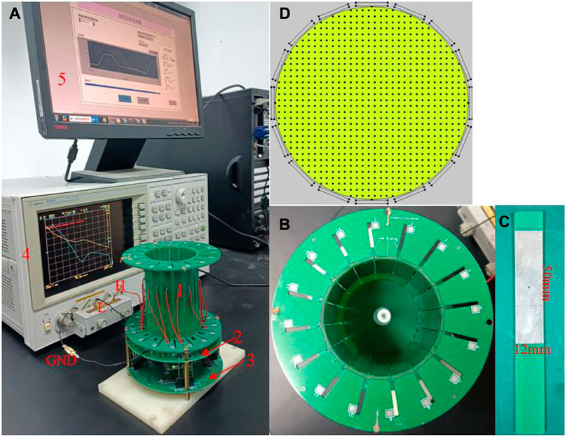
FIGURE 1. Photographs of the ECT measurement system and sensor. (A) Measurement system, (B) ECT sensor, (C) electrode, and (D) pixel points of the imaging area.

FIGURE 2

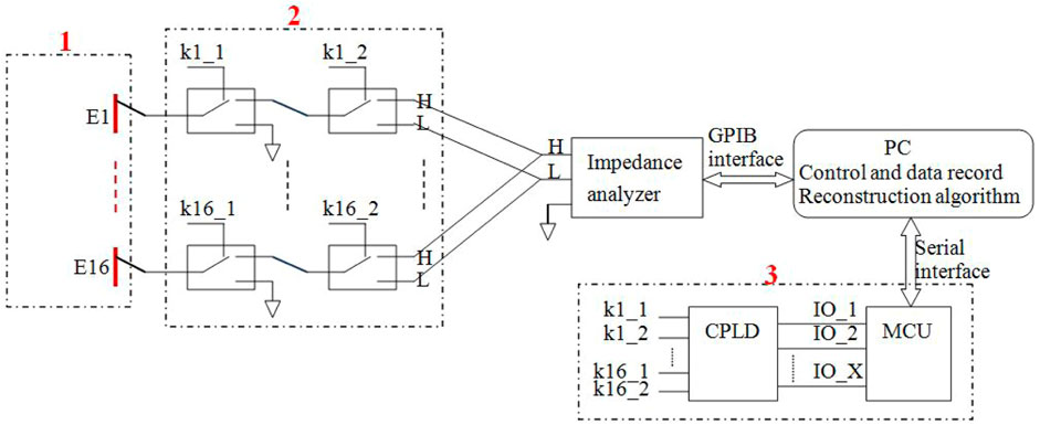
FIGURE 2. Schematic diagram of the electrical connection of the measuring system. The dashed box 1: 16 electrodes. The dashed box 2: The electrical connection of relay circuitry. The dashed box 3: The electrical connection of control circuitry.

The use of electromagnetic relays for electrode switching instead of analog switches is the primary difference between this ECT measuring system and the standard ECT system. The reason for this is that it has been found experimentally that the off-capacitance of the analog switches is very large (several pF–tens of pF) [23], and for a 16-electrode ECT, at least 16 analog switches are required, and the total analog switching circuit forms a stray capacitance of hundreds of pF. When disconnected from the circuit, one opposite electrode pair of the ECT sensor has a capacitance of approximately 0.3 pF; however, when connected to the analog switching circuit, this value would boost to hundreds of pF. The high stray capacitance greatly reduces the measuring accuracy and resolution of the capacitance induced by the object under test. When an electromagnetic relay is in an off condition, the terminals are disconnected physically, leading to a tiny off-capacitance. The capacitance of 120 electrode pairs in this ECT system was measured to be between 8.936 pF and 11.328 pF when the imaging area is empty. When the impedance analyzer was set to its greatest accuracy, the ECT system could achieve a precision of 0.0006 pF. The frequency sweep measurement test reveals that the ECT system has minimal measurement noise between 1 MHz and 10 MHz. The lower the frequency, the greater the noise, and the higher the frequency, the smaller the noise, but if the frequency is too high, the more the ECT system is affected by external interference, considering that the measurement frequency is chosen to be 3 MHz.

2.3 Image reconstruction algorithm

In this paper, we used the traditional conjugate gradient (CG) method for solving the linear inverse problem. The CG method has a fast convergence rate but is only applicable to a linear system of equations with a symmetric positive definite (SPD) coefficient matrix [24]. However, the sensitivity matrix S for the ECT problem is always non-symmetric and ill-conditioned. To obtain a stable solution, it is first necessary to regularize the sensitivity matrix S. Considering$\epsilon \left(x,y\right)$ and $S^{\prime }=\left(S^{T}S+\mu I\right)$, then Eq. 6 can be expressed as [25]

$S^{\prime }·g={\lambda }^{\prime }(7)$

The solution is then solved according to the idea of the CG method.

3 Experimental arrangements

3.1 Simulation arrangement

To check the imaging performance of the ECT sensor and to calculate the sensitivity matrix S (provided for the actual imaging later), simulations were first performed. The simulation was carried out using COMSOL Multiphysics and MATLAB on a PC equipped with an Intel Core i7 processor of 3.40 GHz. First, the same sensor model is created in COMSOL according to the size of the actual ECT sensor in Figure 1. The imaging area is set as a circle with a diameter of 60 mm (as shown in Figure 1D). For the inverse problem, the imaging area is divided into 32 × 32 grids, with the outer part of the circle removed, which results in 812 pixels inside the imaging area. The sensitivity of each of the 812 pixels is then calculated for each electrode pair. The sensitivity was calculated with the imaging zone under the air domain. The sensitivity of electrode pairs i–j at pixel point P (x, y) is shown in Eq. 8, with (E_xi, E_yi) being the x-directional electric field component and the y-directional electric field component at pixel point P when electrode i is used as the excitation electrode and (E_xj, E_yj) are the x-directional electric field component and the y-directional electric field component at pixel P when electrode j is used as the excitation electrode. Each electrode is set in turn as the excitation electrode, and E_x and E_y are calculated for all 812 pixel points. Finally, the sensitivity matrix for all electrode pairs is calculated according to Eq. 8.

$S_{ij}\left(x,y\right)=-E_{xi}\times E_{xj}+E_{yi}\times E_{yj}(8)$

This air domain sensitivity matrix is used for both simulation imaging and later actual imaging. Three simple permittivity distribution models (Figures 3A–C) and two ICH models (I1–I2 in Figure 3) are used for numerical simulation. As for simple models, the background material is air, and the relative permittivity of test objects is 4. The diameter of all the small circles in all simple models is 6 mm. The ICH model is based on the actual brain structure but is simplified by dividing it into five layers from the outside to the inside, simulating skull (rose red), cerebrospinal fluid (brown), gray matter (green), white matter (dark blue), and blood (wine red). The relative permittivity of each part in the ICH model is calibrated to the measured values of human brain tissue from the literature (Table 1). The small red circle in the ICH model is used to represent hemorrhage. The coordinate of the center of the imaging area in I1 or I2 is (0 mm, 0 mm). The small red circle in I1 and I2 represents hemorrhaging in the left hemisphere and right hemisphere, respectively. The diameters of the two small red circles are all 10 mm, and the central coordinates are (−9 mm and 7 mm) and (9 mm and 7 mm), respectively. To image brain hemorrhage, we first subtract the calculated capacitance data of I1 or I2 from the reference data, which are the calculated data with no bleeding present (with the red circles removed and the remainder retained).

FIGURE 3

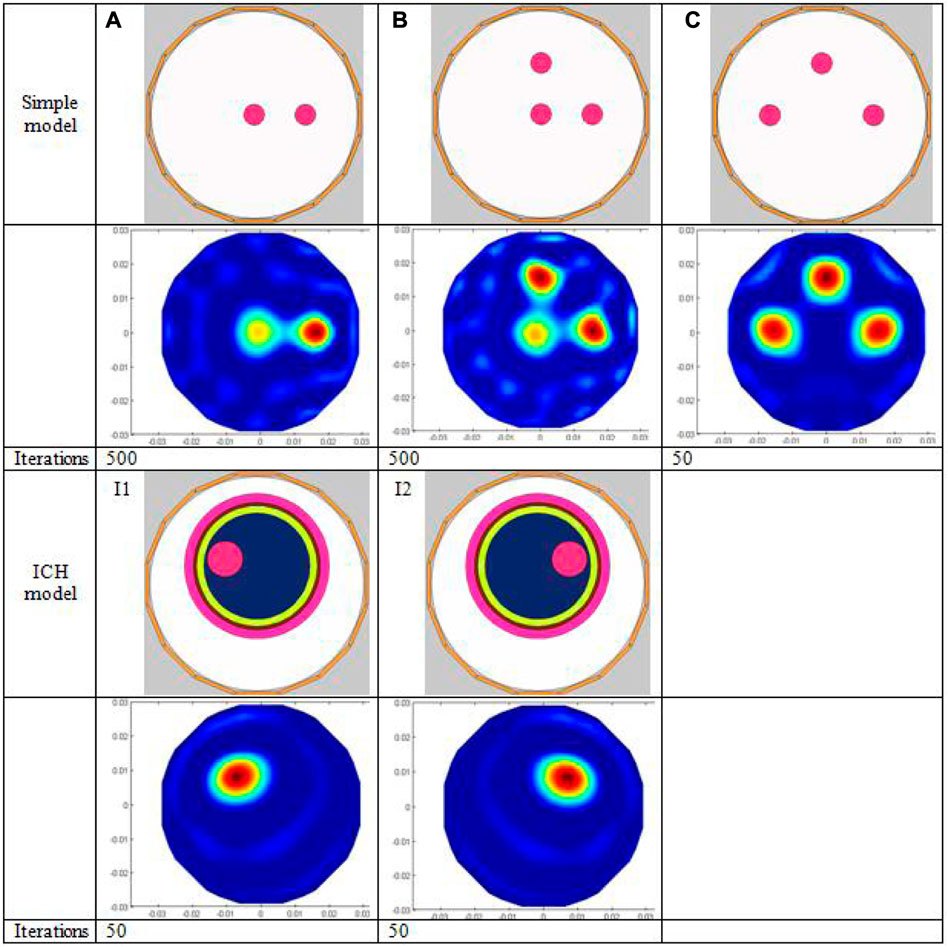
FIGURE 3. Simulation model and imaging results. The first three rows show the simple simulation models (A–C) followed by the corresponding imaging results and the number of iterations; the last three rows show the two ICH models (I1, I2), the corresponding imaging results, and the number of iterations, respectively

TABLE 1

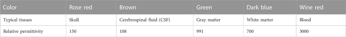
TABLE 1. Relative permittivity of each part in the ICH model (frequency 1 MHz) [11].

To assess the quality of image reconstruction, the relative image error and the correlation coefficient between the true model and reconstructed images are used as criteria. The definition of the relative image error and correlation coefficient is shown in Eqs 9, 10, respectively [21]. The lower the image error and the higher the correlation coefficient mean, the better the image reconstruction results.

$Imageerror=\frac{‖\widehat{g}-g‖}{‖g‖}\times 100\%(9)$

where

$Correlationcoefficient=\frac{{\displaystyle \sum _{i=1}^P}\left(g_i-\overline{g}\right)({\widehat{g}}_i-\overline{\widehat{g}})}{\sqrt{{\displaystyle \sum _{i=1}^P}{\left(g_i-\overline{g}\right)}^2{\displaystyle \sum _{i=1}^P}{\left({\widehat{g}}_i-\overline{\widehat{g}}\right)}^2}}(10)$

is the normalized pixel value reconstructed and g is the normalized permittivity vector of a true distribution in the model. $\widehat{g}$ and $\overline{\widehat{g}}$ are the mean values.

3.2 Actual physical model imaging experiments

As can be seen in Figure 4, the physical model imaging is divided into three parts:Ⅰ, Ⅱ, and Ⅲ. Three models of A1, A2, and A3 in Part Ⅰ are used to image blood at different locations. In models A1 and A2, a plastic tube containing anticoagulant fresh sheep blood (inner diameter 5 mm) is put in the center and 1/2 radius of the imaging region. In A3, two identical blood-filled plastic tubes are positioned at a 1/2 radius apart horizontally. B1, B2, and B3 are three models in Part Ⅱ, in which different solutions are placed in a big cylinder (56 mm inner diameter) and a miniature tube (with a diameter of 10 mm) which is fixed to the position at 1/2 radius of the big cylinder. For B1, water is placed in the large cylinder, while vegetable oil is placed in B2 and B3, and blood is placed inside the small tube for all the three models. First, the big cylinders and small tubes are measured once when empty; the resultant capacitance is used as a reference; next, the cylinders and the small tubes are filled with the appropriate solutions and measured once again; the resulting capacitance is subtracted from the reference capacitance to create an image. Thus, for the B1–B3 model imaging, blood is wrapped in water or vegetable oil. This kind of imaging is a static imaging used mostly to test ECT’s capacity to image targets against complicated backgrounds. Models in Part Ⅲ are C1 –C3. In these models, a tiny tube (inner diameter 8 mm, designated by 1, 2, and 3 in sequence) is positioned within a larger cylinder (inner diameter 56 mm) at 1/2 radius horizontally and vertically. The big cylinder’s is empty inside, devoid of any kind of solution. For C1, all three small tubes are filled with water; for C2, three small tubes 1, 2, and 3 are filled with vegetable oil, alcohol, and blood, respectively; for C3, three small tubes 1, 2, and 3 are filled with alcohol, water, and blood, respectively. With three small tubes filled with air, the subsequent measurement data are utilized as reference data. Part Ⅲ is designed to test the ECT’s capacity to image targets with different relative permittivity. The relative permittivity for all of the solutions employed in physical experiments is listed in Table 2, with blood showing the highest value, followed by water, 75% alcohol, and vegetable oil. Note that the blood used in this work has been diluted with the anticoagulant sodium heparin and that early studies showed that the permittivity of this kind of blood is substantially less than 700 listed in Table 2 but greater than that of water.

FIGURE 4

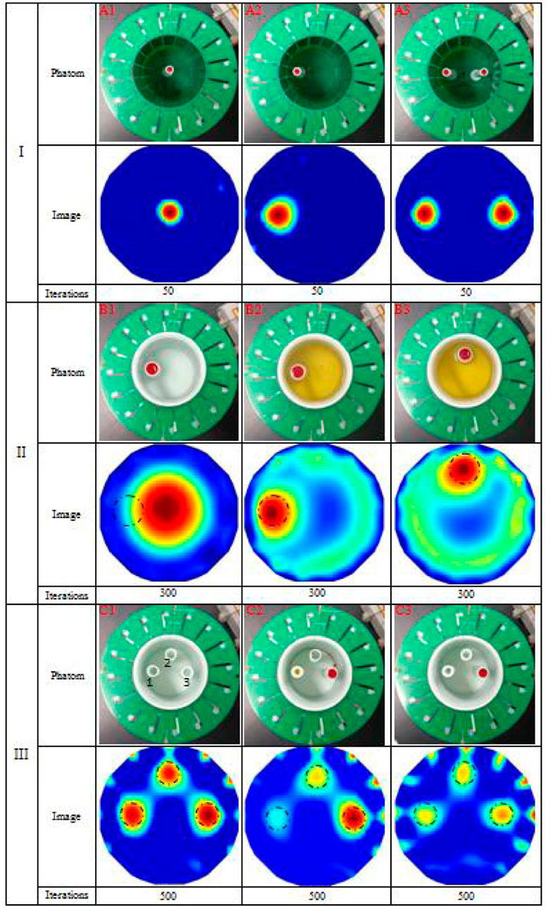
FIGURE 4. Physical experimental models and imaging results.

TABLE 2

TABLE 2. Relative permittivity of the four solutions (frequency 3 MHz).

For imaging of Part Ⅱ and Ⅲ, to quantitatively compare the pixel value levels of the reconstructed image of objects under test, an average pixel value parameter AVP is defined as follows:

$AVP=\frac{{\sum }_{i=1}^P{\widehat{g}}_i}{P}(11)$

For each reconstructed model image, the circular contour of each part image of the object under test was first manually circled, and then the AVP within that contour was calculated as shown in Eq. 11, with $\widehat{g}$ representing the value of each pixel within the contour and P representing the number of pixels within the contour. For B1–B3, the circular contour where the small tube is located is manually circled on each reconstructed image (the diameter being the same for B1–B3), and the AVPs of both the small tube and the remaining part (within the large cylinder) are calculated separately, expressed as AVP_C and AVP_R, respectively, and the ratio of AVP_C: AVP_R is calculated. For C1–C3, the circular contour (with the same diameter), where the three small tubes are located on each reconstructed image, is circled, the AVP of the three small tubes 1, 2, and 3, denoted by AVP₁, AVP₂, and AVP₃, respectively, is calculated, and the ratio of AVP₁: AVP₂: AVP₃ is calculated.

3.3 Isolated porcine brain hemorrhage imaging experiment

To test the feasibility of ECT for imaging actual ICH, we performed ex vivo imaging experiments before conducting animal experiments. The market-bought pig brain in vitro, a 3D-printed big cylinder (56 mm inner diameter) (with a tiny tube of 11 mm inner diameter printed at its inner 1/2 radius), and a syringe with 10 mL of sheep blood diluted with sodium heparin were prepared, as depicted in Figure 5. The pig brain slices were carefully placed into the larger cylinder, equally piled around the small tube, and firmly yet gently squeezed until their height matched that of the electrode. First, the big cylinder containing the pig brain slices was placed in the ECT sensor co-axially and measured once when the small tube is empty, and the resultant capacitance was utilized as the reference data. Then, the blood in the syringe was slowly injected into the small tube. The new capacitance measurement was taken after the small tube was filled. The imaging data are the difference between the reference capacitance and the data with blood injected. The big cylinder was rotated such that the small tube is located at the left of and below the imaging area, and the imaging test for the aforementioned process was carried out at the two positions (as shown in Figure 5), respectively.

FIGURE 5

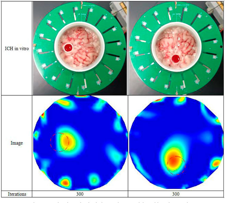
FIGURE 5. Isolated porcine brain hemorrhage models and imaging results.

4 Results and discussion

4.1 ECT measurement noise

The measured capacitance data for the 120 individual electrode pairs with an empty sensor field are shown in Figure 6, with a capacitance distribution ranging from 8.936 to 11.328 pF. This empty field capacitance is very small compared to that of the other ECT system and is entirely due to the use of electromagnetic relays. Figure 7 shows the measured capacitance of an adjacent electrode pair over 2 min, with 2 min being exactly the imaging time of one frame. The standard deviation was calculated to be 0.000127 pF.

FIGURE 6

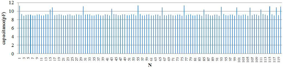
FIGURE 6. Capacitance measurements of 120 independent electrode pairs under an empty field.

FIGURE 7

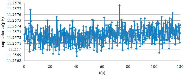
FIGURE 7. Measurement data of one adjacent electrode pair within 2 min.

4.2 Simulation imaging results

Figure 3 displays the simulated imaging results. For simple models A and B, even though all small red circles in the model are set to the same relative permittivity, the pixel value level of the small red circle in the center is substantially lower than that of the small circles positioned at 1/2 radius; thus, the image of the small circle in the center looks a bit hazy. The reason is that the center of the imaging zone for ECT has the lowest sensitivity due to the soft field properties of ECT. Although many advanced reconstruction algorithms in other papers have been found to mitigate this effect successfully, the conjugate gradient approach utilized in this study does not appear to be one of them. The imaging result of simple model C outperforms A and B. Since the radial distance from the center of each of the three smaller circles to the center of the imaging zone is the same (1/2 of the larger circle’s radius), the pixel values for each of the smaller circles are roughly the same. The number of iterations in the reconstruction of models A, B, and C are 500, 500, and 50, respectively. For the images of models A and B, the white spot of noise is considerably more pronounced than in the image of model C since the sensitivity of the center is the lowest, and a very high number of iterations are required to show the small circle in the middle. With model C, a decent reconstructed image can be obtained only after 50 iterations. Table 3 displays the image error (%) and the correlation coefficient of all models’ imaging; the image error (%) of model AB is higher than that of model C, and the correlation coefficient is lower for model AB. The imaging of ICH models I1 and I2 is clear, and the location and size of the hemorrhage are more accurately reflected due to the use of time-difference imaging in large part, in which data calculated with the hemorrhage circle existed is subtracted from data calculated with the hemorrhage circle removed. Second, the diameter of the small red circle in the ICH model is larger than that in the simple model. On the other hand, it shows that ECT can image targets behind multiple layers of material.

TABLE 3

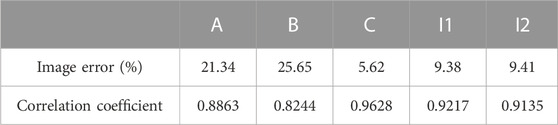
TABLE 3. Image error (%) and correlation coefficient for simulation results.

4.3 Physical experimental imaging results

Figure 4 displays the imaging outcomes of the physical experiments. Models A1–A3 in Part Ⅰ exhibit excellent results. The location of the blood in the image is spotted with its location in the model. Nonetheless, the unequal distribution of sensitivity in the imaging area contributes to a much smaller diameter of the blood image in A1 compared to A2 and A3. The imaging of the same object placed in the center has the lowest sensitivity; thus, its image appears smaller than that of the same object placed in other positions. In most cases, ECT can image blood.

The imaging results of models B1–B3 in Part Ⅱ is significantly poor. The results of B2 and B3 can still reflect the position and size of blood, but the backdrop appears as huge plaques, mainly because blood is surrounded by other high permittivity backgrounds (not air); thus, it belongs to static imaging rather than differential imaging. The B1 imaging results do not show the presence of the blood portion at all. This is mainly because blood is surrounded by water, and the permittivity of this blood diluted with sodium heparin is not much larger than that of water, as already described. The diameter of tubular blood is only 10 mm, which is only 1/6 of the diameter of water, so the change in capacitance caused by the blood part is very small and submerged in the capacitance change caused by water. Thus, it is difficult to show the presence of blood in the reconstructed image. Images of B2 and B3 show the presence of the blood component, and their location and size are very close to the real model. In addition, part of the reason is that the background of blood wrapped in B2 and B3 is replaced by vegetable oil, and the relative permittivity of vegetable oil is less than 4 (Table 2), which is much smaller than that of blood. For this reason, the imaging can emphasize the existence of the blood portion even though the diameter of tubular blood is much smaller than that of vegetable oil due to the substantial difference in relative permittivity. However, for imaging of models B2 and B3, a large area of plaque appeared in the background outside of the blood image, with areas of low pixel values appearing in the middle near the blood and areas of higher pixel values appearing near the electrode. On the one hand, this is still caused by uneven sensitivity of the imaging area, and on the other hand, it is because the soft field characteristic of ECT will cause the sensitivity distribution of the imaging area to change with the distribution of materials with multiple different permittivities. Table 4 gives the ratio of the average pixel values of the blood area and the remaining background in B2 and B3 images, which is expressed as AVP_C: AVP_R. The ratio of B2 and B3 is closer because in B2 and B3 only the position of blood is different and the rest of the conditions are identical. The average value of B2 and B3 is 51.93:1, which also indirectly reflects that the permittivity of blood is much higher than that of vegetable oil; however, it will not be equal to the actual permittivity ratio of blood to vegetable oil because the imaging will be affected by the volume and position of the objects besides permittivity. The average pixel value ratio in the image of B1 was not determined since blood could not be imaged. This experiment demonstrates that it is exceedingly difficult to conduct static imaging on an object with complex backgrounds with minor changes in permittivity, a recurring bottleneck in the field of electrical tomography.

TABLE 4

TABLE 4. Average pixel value ratio of blood to the background for imaging results in Part Ⅱ.

The imaging findings of C1–C3 in Part Ⅲ reveal the presence of three tubes of solution more clearly, although there are numerous high-pixel-value patches near the electrodes, which is primarily caused by the noise being increased as a result of the high number of iterations in image reconstruction. For C1, the three tubes are all filled with water and positioned at the same distance from the center, so the images of the three tubes with solution should theoretically be identical. The image of C1 shows that the three tubes’ pixel values are roughly comparable. The average pixel value ratio of the three tubes is given in Table 5 as AVP₁: AVP₂: AVP₃ = 1:0.91:1.24, which are close to each other, and the subtle differences may be caused by differences in the placement of the large cylinders. Due to the manual placement of the big cylinder, the center axis of the large cylinder does not exactly coincide with the center axis of the imaging area; therefore, there is a distance discrepancy between the centers of the three tubes and the center of the imaging area. The imaging of C2 reveals three circular regions ranging in color intensity from light to dark from left to right. The solutions in 1, 2, and 3 tubes in C2 are vegetable oil, alcohol, and blood in the order of increasing permittivity, which correlates to the color depths of the three tubes’ imaging areas. In Table 5, the ratio of the average pixel values for the three tubes of solutions of C2 is 1:21.82:158.67. Even though the ratio of the average pixel values of the three tubes does not match the ratio of the permittivity values of the three solutions as shown in Table 2, the size pattern is consistent. The discrepancies between the color depths of the three tube locations in the image of C3 are minute. Table 5 provides the average pixel value ratio of 1:1.18:1.45 for the three tube regions in C3 imaging, which grows steadily although the difference is similarly minimal. Also, 1, 2, and 3 tubes in C3 are filled with alcohol, water, and blood solutions, respectively. The relative permittivity of alcohol and water is 40 and 80, respectively, and that of blood is somewhat more than that of water. The ratio of permittivity of the three solutions climbs progressively from tiny to large, mirroring the ratio of the three tubes’ average pixel values. Nevertheless, the average pixel value ratio of the three tubes in C3 is significantly lower than that in C2, as evidenced by the images’ color tones. Because vegetable oil has a permittivity of 2–4, the contrast between the permittivity of vegetable oil, alcohol, and blood in C2 is larger than that of alcohol, water, and blood in C3. The three-part physical experiment demonstrates that our developed ECT system is capable of imaging blood, with the pixel values reflecting the varied permittivity distributions.

TABLE 5

TABLE 5. Average pixel value ratio of the three tube solutions for imaging results in Part Ⅲ.

4.4 Experimental results of brain hemorrhage imaging on isolated pigs

Figure 5 depicts the results of isolated porcine brain hemorrhage imaging tests. The red dashed circles in Figure 5 depict the real blood position. Although the imaging results can approximate the presence of blood, they deviate from the actual blood position. No matter whether blood was at 1/2 of the radius at the left or below in the actual situation, the imaging results deviated by about 3 mm from the center of the imaging area. In addition to the blood image area, there are other small regions with high pixel values in the images, notably around the electrodes. The most probable explanation for this is that the permittivity of blood is slightly larger than that of the isolated porcine brain and hence does not crush it. This effect is primarily attributable to the frozen porcine brain that was thawed and then doped with melt water, resulting in the porcine brain’s permittivity being drastically lowered. Thus, the actual difference of permittivity between pig brain and blood is minimal. Second, the pig brain belongs to the non-uniform dielectric distribution, which contains gray matter, white matter, cerebrospinal fluid, and a small amount of residual blood, so it is in homogeneous medium, thus leading to a large difference between the sensitivity distribution of the imaging area full of pig brain and full of air, and the sensitivity matrices used for imaging in this paper are all calculated when the imaging zone is full of air, leading to poor imaging of blood, which may also be the reason why the imaging results deviate from the actual location. Nevertheless, the imaging results reveal the presence of blood more distinctly. Since the permittivity of the plastic cylinder material is very small and the permittivity of the actual skull is smaller than that of other brain tissues, the large cylinder wall can be regarded as the skull, so that the ex vivo experimental model can be approximately equivalent to the structure of an actual human head; thus, this ex vivo pig brain hemorrhage imaging experiment demonstrates the feasibility of the technique.

5 Conclusion

Extremely high morbidity and mortality rates are associated with ICH, and early detection and treatment are the keys to reducing mortality and enhancing postoperative results. In addition, currently, there is no portable and diminutive brain hemorrhage detection gadget. In this study, we constructed a 16-electrode ECT system based on an impedance analyzer and proved its viability for imaging brain hemorrhage by means of numerical simulation and physical measurements. In the simulation tests, a five-layer spherical brain hemorrhage model was created, and the imaging results precisely depicted the location and size of the hemorrhage. In physical studies, an isolated pig brain hemorrhage model was created and measured by the developed ECT system for differential imaging; the imaging findings similarly demonstrated the existence of brain hemorrhage, although the location of the hemorrhage in the image was somewhat altered relative to the actual position. In conclusion, the results of the simulation and the ex vivo imaging experiments confirmed the feasibility of ECT for brain hemorrhage imaging; however, the accuracy and resolution of the imaging were not high enough to be used for actual brain hemorrhage imaging. Therefore, improvements are required. The subsequent stage is to initially enhance the ECT system’s performance. Second, a more advanced imaging algorithm should be developed to address the issue of imaging bias in ex vivo research. Additionally, ICH imaging tests in vivo should be conducted to examine the efficacy of ECT in actual hemorrhage imaging.

Data availability statement

The original contributions presented in the study are included in the article/supplementary, material, further inquiries can be directed to the corresponding authors.

Author contributions

GJ: methodology and ECT system design; RX and WZ: hardware design, simulation experiments, and physical experiments; ZB: algorithmic design; GJ and NL: writing—reviewing and editing.

Funding

This research was funded by the Foundation of Scientific and Technological Innovation Capability Promotion of the Army Medical University (2019XQY06).

Conflict of interest

The authors declare that the research was conducted in the absence of any commercial or financial relationships that could be construed as a potential conflict of interest.

Publisher’s note

All claims expressed in this article are solely those of the authors and do not necessarily represent those of their affiliated organizations, or those of the publisher, the editors, and the reviewers. Any product that may be evaluated in this article, or claim that may be made by its manufacturer, is not guaranteed or endorsed by the publisher.

References

1. Collaborators GBDS, Global, regional, and national burden of stroke, 1990-2016: A systematic analysis for the global burden of disease study 2019. Lancet Neurol (2021) 18, 439–58.

Google Scholar

2. Wang L, Liu J, Yang G, Peng B, Wang Y. The prevention and treatment of stroke in China is still facing great challenges—summary of China stroke prevention report 2018. Chin Circ J (2019) 34(02):6–20.

Google Scholar

3. AyazLzzetogluIzzetoglu HMK, Onaral B, Ben Dor B. Early diagnosis of traumatic intracranial hematomas. J Biomed Opt (2019) 24(5):1. doi:10.1117/1.jbo.24.5.051411

CrossRef Full Text | Google Scholar

4. Balami JS, White PM, McMeekin PJ, Ford GA, Buchan AM. Complications of endovascular treatment for acute ischemic stroke: Prevention and management. Int J Stroke (2018) 13(4):348–61. doi:10.1177/1747493017743051

PubMed Abstract | CrossRef Full Text | Google Scholar

5. BodensteinDavidMarkstaller MMK. Principles of electrical impedance tomography and its clinical application. Crit Care Med (2010) 37(2):713–24. doi:10.1097/CCM.0b013e3181958d2f

CrossRef Full Text | Google Scholar

6. Griffiths H. Magnetic induction tomography[J]. Meas Sci Tech (2001) 12:1126. doi:10.1088/0957-0233/12/8/319

CrossRef Full Text | Google Scholar

7. Braun F, Proena M, Lemay M, Limitations and challenges of EIT-based monitoring of stroke volume and pulmonary artery pressure[J]. Physiol Meas (2018) 39(1):014003. IOP Publishing. doi:10.1088/1361-6579/aa9828

PubMed Abstract | CrossRef Full Text | Google Scholar

8. Toivanen J, Hnninen A, Savolainen T, Monitoring hemorrhagic strokes using EIT[J] (2021).

Google Scholar

9. Mcdermott B, Elahi A, Santorelli A, O’Halloran M, Avery J, Porter E, Multi-frequency symmetry difference electrical impedance tomography with machine learning for human stroke diagnosis. Physiol Meas (2020) 41(7):075010 doi:10.1088/1361-6579/ab9e54

PubMed Abstract | CrossRef Full Text | Google Scholar

10. Watson S, Williams RJ, Griffiths H, A transceiver for direct phase measurement magnetic induction tomography[C]//International Conference of the IEEE Engineering in Medicine and Biology Society. In: Proceeding of the Engineering in Medicine and Biology Society, 2001. Proceedings of the 23rd Annual International Conference of the IEEE. IEEE (2001).

Google Scholar

11. Gabriel S, Lau RW, Gabriel C, Gabriel S, Lau RW, The dielectric properties of biological tissues: II. Measurements in the frequency range 10 Hz to 20 GHz. Phys Med Biol (1996) 41(11):2251–69. doi:10.1088/0031-9155/41/11/002

PubMed Abstract | CrossRef Full Text | Google Scholar

12. Be Z, Ya Q, Li G, Detection of rabbit intracranial hemorrhage based on permittivity[J]. Meas Sci Tech (2019)(11) 30.

Google Scholar

13. Bai Z, Li H, Chen J, Zhuang W, Li G, Jin G, et al. Research on the measurement of intracranial hemorrhage in rabbits by a parallel-plate capacitor. PeerJ (2021) 9(99):e10583. doi:10.7717/peerj.10583

PubMed Abstract | CrossRef Full Text | Google Scholar

14. Rashid WNA, Johana Rahim E, AbdulAbdullah R, Jaafar A, Mohmad HL. Electrical capacitance tomography: A review on portable ECT system and hardware design[J]. Sensor Rev (2016) 36(1).

Google Scholar

15. Warsito W, Marashdeh Q, Fan LS. Electrical capacitance volume tomography. IEEE Sensors J (2007) 7(4):525–35. doi:10.1109/jsen.2007.891952

CrossRef Full Text | Google Scholar

16. WangYang HW. Application of electrical capacitance tomography in pharmaceutical fluidised beds – a review. Chem Eng Sci (2020) 231:116236. doi:10.1016/j.ces.2020.116236

CrossRef Full Text | Google Scholar

17. Taruno WP, A novel sensor design for breast cancer scanner based on electrical capacitance volume tomography (ECVT). IEEE Sensors (2012) 1 – 4.

PubMed Abstract | CrossRef Full Text | Google Scholar

18. Taruno WP, Brain tumor detection using electrical capacitance volume tomography. In: 6th International IEEE/EMBS Conference on Neural Engineering (NER) (2013). 743–6.

Google Scholar

19. Taruno WP, Electrical Capacitance Volume Tomography for human brain motion activity observation. In: Proceeding of the Middle East Conference on Biomedical Engineering (MECBME) (2014). 147–50.

CrossRef Full Text | Google Scholar

20. Yang W. Q., Peng L Image reconstruction algorithms for electrical capacitance tomography[J]. Meas Sci Tech 2003(1):14.

Google Scholar

21. Ye J, Wang H, Yang W. Image reconstruction for electrical capacitance tomography based on sparse representation[J]. IEEE Trans Instrumentation Meas (2014) 64(1):89–102.

Google Scholar

22. Cui Z, Qi W, Qian X, Fan W, Zhang L, Yang W, et al. A review on image reconstruction algorithms for electrical capacitance/resistance tomography. Sensor Rev (2016) 36(4):429–45. doi:10.1108/sr-01-2016-0027

CrossRef Full Text | Google Scholar

23. Yusuf A, Harry SS, Sudiana D, Tamsir AS, Widada W, Taruno WP, et al. Switch configuration effect on stray capacitance in electrical capacitance volume tomography hardware[J]. TELKOMNIKA (Telecommunication Computing Electronics and Control) (2016) 14(2):456. doi:10.12928/telkomnika.v14i2.3328

CrossRef Full Text | Google Scholar

24. Axelsson O. Iterative solution methods. Cambridge: Cambridge University Press (1994).

Google Scholar

25. Yu C, Han J, Song Y, Liu W A novel conjugate gradient image reconstruction algorithm for electrical capacitance tomography system[C]//. In: Proceeding of the International Conference on Challenges in Environmental Science and Computer Engineering. IEEE (2010).

Google Scholar