Physics informed neural networks for phase field fracture modeling enhanced by length-scale decoupling degradation functions

The paper proposed a novel framework for efficient simulation of crack propagation in brittle materials. In the present work, the phase field represents the sharp crack surface with a diffuse fracture zone and captures the crack path implicitly. The partial differential equations of the phase field models are solved with physics informed neural networks (PINN) by minimizing the variational energy. We introduce to the PINN-based phase field model the degradation function that decouples the phase-field and physical length scales, whereby reducing the mesh density for resolving diffuse fracture zones. The numerical results demonstrate the accuracy and efficiency of the proposed algorithm.

1 Introduction

Predicting material and structural failure due to crack nucleation and extension is central to many engineering applications. Several numerical methods are developed to capture complex fracture phenomena, such as the finite element method [1], the boundary element method [2], the cohesion zone method [3,4], the extended finite element methods [5], the peridynamics Ha and Bobaru [6] and the phase field methods. In these methods, the phase field method has demonstrated advantages in description of complex fracture patterns. By introducing additional continuous field variables to track discrete discontinuities with diffuse fracture zones, the phase field method Bourdin et al. [7] unifies crack initiation, propagation, branching, and merging in structures.

In phase field method, the diffuse fracture region must be resolved with sufficient degrees of freedom to obtain an accurate solution. The length scale of the physical process zone is proportional to the ratio of the fracture energy to the square of the material strength. For most problems modeled by linear elastic fracture mechanics, the length scale of the physical process zone is very small compared to structures, but the commonly used formulas in fracture phase field approach does not distinguish between the phase field crack length scale the physical process zone length scale, which leads to prohibitive meshing requirement when extending the models with nanoscale phase field length to large structures. To alleviate the meshing burden, Wu et al. proposed a length-scale insensitive phase-field model [8], but the method is practically applicable to the scenario that the phase-field length scale and physical process zone length scale are in the same order of magnitude. Lo et al. [9] proposes a degradation function that separates the phase field length scale from physical length-scale, which enables one to simulate crack propagation in large scale structures.

As a branch of artificial intelligence, the deep learning based on Artificial Neural Networks has made tremendous progress with the explosive growth of data in the past decade [10–12] and applied in a wide range of areas. ANN were initially trained for Computer Visualization and Natural Language Processing tasks [13,14]. When it comes to the field of physical simulation, two major problems arise: firstly, it is cumbersome to obtain the data from complex engineering systems; secondly, the result predicted by the training data cannot ensure that the physical principles of the problem are satisfied. Hence, the effectiveness and reliability of ANN in characterizing physical phenomena are questionable. To overcome the difficulties, physics informed neural networks (PINN) [12,15–19] were put forward, which comply with the distribution of the training data as much as possible and meanwhile obey the laws of physics which are commonly formulated by partial differential equations. Compared to purely data-driven neural network learning, PINN allows learning with fewer data samples and obtaining models with greater generalization capability. Goswami et al. [20], Goswami et al. [21] firstly applied PINN to solve the phase field model for simulating the growth and propagation of fractures in brittle materials. Their results offer improved accuracy and efficiency, demonstrating the advantages of PINN in simulating moving boundary problems.

In the present work, we introduce the degradation function proposed by Lo et al. [9] to the PINN-based phase field method [20,21], in order to analyse crack growth in large structures with a data driven and mechanism based hybrid approach. We use three numerical simulation examples to demonstrate that the physical neural network combined with the proposed degradation function is correct and advantageous. The remaining o the paper is organized as follows. Section 2 introduces fracture phase field method and shows how the phase field length scale and the physical process zone length are decoupled. Section 3 elaborates on how the fracture phase field model is discretized with the PINN. The numerical examples are given and analysed in Section 4, and Section 5 is the conclusion and outlook of future work.

2 Phase field model of cracks

2.1 Conventional phase field crack modeling

The phase-field crack modeling of brittle fractures involves the integration of two fields: the elastic field u and the phase field d, and the crack propagation is determined according to the free energy minimization principle. Based on the energy decomposition proposed by Francfort and Marigo [22], the free energy of the fracture system is given as:

$E\left(u,\mathrm{\Gamma }\right)={\int }_{\mathrm{\Omega }}{\psi }_e\left(\epsilon \left(u\right)\right)\mathrm{d}x+G_c{\int }_{\mathrm{\Gamma }}\mathrm{d}s(1)$

where: G_c is the critical energy release rate, ψ_e is the elastic energy density, Γ is the fracture surface, and Ω is the problem domain. The right hand side of the equation is the sum of the elastic strain energy and the fracture surface energy, and the fracture phase field method in mechanics assumes that the crack should follow the direction of minimum free energy and be irreversible.

Since the boundary integral involved in the surface energy is not easy to handle, it is replaced by the crack density equation in the following:

${\psi }_c=\frac{G_c}{2l_0}\left(d^2+l_0^2|▽d{|}^2\right)(2)$

where: d is the order parameter; l is the diffuse crack width. Theoretically, the model draws on the elliptic regularization method of the Mumford-Shah generalization Lie et al. [23] in computer image segmentation (hence the model is also known as AT2).

Since the elastic strain energy cannot distinguish between positive and negative for stress and strain, Amor et al. [24] and Miehe et al. [25] proposed a tension-compression split of the elastic strain energy, which is defined as:

${\psi }_e\left(\epsilon ,d\right)=g\left(d\right){\psi }_e^{+}+{\psi }_e^{-}(3)$

where the elastic energy is determined by both the strain and the order parameter d. g(d) represents the degradation function, which is used to reduce the strength of material around the cracked region. To model material failure and crack propagation, the material should be fully elastic when it is intact and disappears when it is completely cracked. This is achieved by multiplying the elastic energy by the degradation function in the phase field description of the damaged materials.

In addition, to prevent the release of elastic energy after unloading from causing crack healing, Miehe et al. [26] proposed a very concise and effective solution by introducing a historical strain function:

$H\left(x,t\right)=\underset{\tau \in \left[0,t\right]}{\mathrm{m}\mathrm{a}\mathrm{x}}{\psi }_e^{+}(4)$

Eq. 4 indicates that the crack driving force is taken as the historical maximum tensile elastic energy. Even after re-unloading, the tensile elastic energy maintains its maximum value and thus prevents crack healing.

Substituting the crack density in Eq. 2 and the elastic energy in Eq. 5 into the free energy of the fracture system in Eq. 1:

$E\left(u,d\right)=g\left(d\right){\psi }_e^{+}+{\psi }_e^{-}+\frac{G_c}{2l}\left(d^2+l^2{\left|▽d\right|}^2\right)+g\left(d\right)H\left(x,t\right)(5)$

Finally, we seek the solution to minimize the free energy E, which consists of the elastic strain energy ψ_e and the fracture surface energy ψ_c.

2.2 Degradation function

The degradation function needs to satisfy the following conditions:

$\begin{array}{c}\hfill g\left(1\right)=1\\ \hfill g\left(0\right)=0\\ \hfill g_{\prime }\left(0\right)=0\end{array}(6)$

The most widely used degradation function in the literature is a quadratic function,

$g\left(d\right)={\left(1-d\right)}^2.(7)$

With this degradation function, for the AT2 model (d²) with uniform uniaxial tension, the peak stress is obtained as:

${\sigma }_c=\sqrt{\frac{27G_{c}E}{256l_0}}(8)$

Eq. 8 shows that the phase-field length, l₀ is not an independent parameter but dependent on the material strength, σ_c, fracture energy, G_c, and Young’s modulus, E. This length scale, which represents the size of the physical process zone, l_p, can be quite small for real materials. In the past, the typical approach has been to set l_p equal to l₀. However, this means that numerical solutions must have the ability to resolve the small l_p, which can be a challenge for large engineering structures. This is because the mesh size around cracks must be a fraction of l₀, at most l₀/2, leading to computationally intensive simulations. To overcome the difficulties, Lo et al. [9] proposed a new degradation as:

$g\left(d\right)=q\ast \left[1-{\left(\frac{q-1}{q}\right)}^{{\left(1-d\right)}^2}\right](9)$

This degradation function meets all the requirements of Eq. 6. Its shape depends on the value of q. When q is 200, the shape of the proposed degradation function in Eq. 23 is close to that of the classical degradation function in Eq. 7. When the value of q is slightly larger than 1, the shape of the degradation function g(d) will dramatically alter following marginal change of the value of q. This can be seen in Figure 1.

FIGURE 1

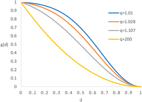
FIGURE 1. Shape of the proposed degradation function in this work. As the parameter q increases the degradation function approaches the standard quadratic, and as q decreases towards 1 the peak stress predicted by the model increases.

The peak stress for a bar under homogeneous uniaxial tension can be determined using the proposed degradation function, as follows:

${\sigma }_c^{\ast }=\frac{\sqrt{\frac{27G_{c}E}{256l_0}}}{\sqrt{\left(q-1\right)\ln \left(\frac{q}{q-1}\right)}}(10)$

It’s worth mentioning that we’ve introduced the notation ${\sigma }_c^{*}$ to represent the peak stress calculated using the alternative degradation function, differentiating it from the conventional peak stress (σ_c). Additionally, the physical length scale l_p in the case of the alternative degradation function is given as:

$l_p=\left(q-1\right)\ln \left(\frac{q}{q-1}\right)l_0.(11)$

This allows us to also express the peak stress with the proposed degradation function as follows:

${\sigma }_c^{\ast }=\sqrt{\frac{27G_{c}E}{256l_p}}(12)$

q can be used to maintain the same peak stress ${\sigma }_c^{*}$ in numerical simulations with the increase of the phase-field length, which allows for a coarser mesh in the proximity of cracks. Supposing G_c, E, and ${\sigma }_c^{*}$ are given as constants, when q is large, the sizes of the physical process zone, l_p, and the phase-field process zone, l₀, are comparable. Moreover, the finite element mesh must be refined according to l₀. If we would like to increase the l₀ by 4 times without changing the peak stress, ${\sigma }_c^{*}$ or the l_p. q needs to be 1.107 according to Eq. 10. If we aim to increase the length scale l₀ by 16 times while still maintaining the same peak stress, we find that q ≈ 1.0148. If we increase l₀ by 100 times, we find that q ≈ 1.00155. This demonstrates that the proposed degradation function allows for decoupling l₀ from l_p. Note that these results assume homogeneous post-peak behavior and that localized deformations have been suppressed. Importantly, it’s worth noting that the resulting peak stress remains the same for different phase-field length scales. Also note that the material is not damaged, i.e., d begins to increase from 0, until the strains exceed peak strains.

3 PINN-based fracture phase-field modeling

This section details the implementation of the phase field method based on PINN [20, 21]. Firstly, the deep neural network will be described, and secondly, the synthesis between the PINN phase field method with the degradation function mentioned in the above section is explained.

3.1 Deep neural networks

Deep learning is a branch of machine learning based on deep neural networks. In comparison with shallow neural networks, deep learning has more hidden layers and is more capable of fitting non-linearities. Neural network training consists of two steps, i.e., forward propagation and backward propagation. The forward propagation is used to train the neural network parameters, while the backward propagation is used to update the neural network parameters and find the optimal solution. In this paper, a feed-forward deep neural network is used for the study. The hidden layer of the deep neural network contains its main parameter weights W and biases b, and the parameters are continuously optimized by optimization algorithms (e.g., adaptive moment estimation (ADAM), proposed Newton method (L-BFGS), etc.) to find the optimal solution. Supposing that the network consists of L hidden layers, with layer 0 denoting the input layer and layer (L + 1) denoting the output layer, the expression of the neural network can be written as:

$z_i^l={\sigma }_{l-1}\left(\sum _{j=1}^{m_{l-1}}\left(W_{i,j}^l\left(z_j^{l-1}\right)+b_i^l\right)\right)(13)$

The calculation of the output Y in the feed-forward algorithm can be represented as follows: the activation function σ_l−1 in layer l is used in conjunction with the number of neurons m_l−1 in layer l − 1.

$\begin{array}{ccc}\hfill Y_l\hfill & \hfill =\hfill & \hfill {\sigma }_l\left(W_{l+1}{z}_l+b_{l+1}\right),\hfill \\ \hfill z_l\hfill & \hfill =\hfill & \hfill {\sigma }_{l-1}\left(W_l{z}_{l-1}+b_l\right),\hfill \\ \hfill z_{l-1}\hfill & \hfill =\hfill & \hfill {\sigma }_{l-2}\left(W_{l-1}{z}_{l-2}+b_{l-1}\right),\hfill \\ \hfill \hfill & \hfill \dots \hfill \\ \hfill z_1\hfill & \hfill =\hfill & \hfill {\sigma }_0\left(W_{1}x+b_1\right)\hfill \end{array}(14)$

where x represents the input to the neural network in Eq. 14. Forward propagation is used to train the neural network parameters, (w, b), which represent all the W_l and b_l parameters that appear in Eq. 14. We evaluate a neural network prediction result by the loss function, and if the loss value reaches low enough, (which is generally not possible to be 0) we end the neural network training. The common loss functions for regression are MAE loss, MSE loss, and smooth L1 loss. Their expressions are given by the following equations.

$L=\frac{1}{n}\sum _{i=1}^n\left|Y_i-N\left(x_i;W,b\right)\right|(15)$

$L=\frac{1}{n}\sum _{i=1}^n{\left(Y_i-N\left(x_i;W,b\right)\right)}^2(16)$

$\mathrm{s}\mathrm{m}\mathrm{o}\mathrm{o}\mathrm{t}\mathrm{h}{\mathrm{L}}_{\mathrm{1}}\left(x\right)=\left\{\begin{array}{cc}0.5{\left(Y_i-N\left(x_i;W,b\right)\right)}^2\hfill & \mathrm{i}\mathrm{f}|Y_i-N\left(x_i;W,b\right)|<1\hfill \\ |Y_i-N\left(x_i,W,b\right)|-0.5\hfill & \mathrm{o}\mathrm{t}\mathrm{h}\mathrm{e}\mathrm{r}\mathrm{w}\mathrm{i}\mathrm{s}\mathrm{e},\hfill \end{array}\right.(17)$

Y_i represents the target value and N(x_i; W, b) represents the predicted value of the neural network. Backward propagation is automatically performed based on the value of the loss function. Automated differentiation and weight update implemented in TensorFlow or PyTorch allow algorithm designers to perform their tasks without coding the back propagation from scratch. The reader is referred to LeCun et al. [27] for details of the adopted gradient calculation method and the layer-by-layer chain rule gradient derivation process. In the following section we focus on an algorithmic approach for solving problems using the variational energy-based physics informed neural network.

3.2 Variational energy based PINN

We can define the problem by a one-dimensional time-independent differential equation:

$F\left(u,u_x,\dots ,u_{x\dots x},x,f\left(x\right)\right)=0,(18)$

together with the Dirichlet boundary condition, which is defined as:

$u\left(x_D\right)=u_D(19)$

The deep neural network can be utilized to compute the field variable, represented by u, by considering variables such as the Dirichlet boundary point, represented by x_D, and the source term, represented by f(x). Furthermore, the first, second, and higher-order derivatives with respect to the independent variable x can be calculated using u_x, u_xx and u_x…x respectively. The variational energy principle has the distinctive benefit of automatically satisfying homogeneous Neumann boundary conditions. At this point, the expression for the variational energy is:

$V={\int }_{\mathrm{\Omega }}y\left(u,u_x,\dots ,u_{x\dots x},x,f\left(x\right)\right)d\mathrm{\Omega }(20)$

where y is the differentiable functional. Ω is the problem domain for which a solution is required, so the problem for which we require a solution can be expressed as follows:

$\begin{array}{cc}\hfill \hfill & \hfill u^{*}={\mathrm{argmin}}_{u}V\left(u\right)\hfill \\ \hfill \text{subject\hspace{0.17em}\hspace{0.17em}to}:\hfill & \hfill u\left(x_D\right)=u_D.\hfill \end{array}(21)$

The steps for solving the differential equation using a neural network are detailed as follows: First, we construct a neural network, N(x; W, b) with initial parameters. Second, we revise the neural network according to the boundary conditions. In terms of addressing the boundary conditions in the context of neural network, weak form and the strong form. When dealing with boundary conditions in a weak form, a penalty term reflecting the boundary condition is added to the loss function. But this may cause interference among different loss terms, which slows or even cripples the convergence of the problem. So, we prefer the strong form here and we redesign the output of the neural network so as to comply with the Dirichlet boundary condition.To this end, we set:

$u\approx {\tilde{u}}_D+B\left(x\right)\cdot N\left(x;W,b\right).(22)$

The function ${\tilde{u}}_D$ is selected such that it matches the value of u_D at the Dirichlet boundary points. Meanwhile, B(x) is equal to zero at the same boundary. There is no requirement for a boundary component in the calculation of the loss function. Thirdly, the output of the neural network existing in variable energy expression is calculated using an automatic differential technique. Having computed the first and higher-order derivatives of u, we can now calculate the variational energy at each quadrature point. This is done by using u_x from Eq. 22 and its derivatives obtained previously. The total variational energy of the system is then obtained by summing the energies at each point, as defined in Eq. 20. In this step we use the PDE (partial differential equation), i.e., the total variational energy, as the loss function of the neural network. The neural network constructed above is named physics informed neural network. The final step is to update the neural network parameters W and b by adjusting them so that the next neural network output value is closer to the target value.

According to the above steps, Goswami et al. [20], Goswami et al. [21] proposed a PINN combined with phase field method to simulate the fracture problem. The displacement control is applied for the loading process. To train the PINN, a fixed displacement step, denoted by △u, is taken and the strain-history function is updated at each displacement increment. Before training the network, the weights are initialized randomly from a Gaussian distribution with the Xavier initialization technique [11]. In order to calculate the parameters of the neural network at the first displacement step i, the Gaussian quadrature points and their corresponding weights are generated using the above process, and in the subsequent step, the automatic differentiation method is employed to calculate the displacement increment, △u, and the eigenvalues of the strain, (λ₁, …, λ_d), where d denotes the number of spatial dimensions. These eigenvalues are then utilized to determine ${\psi }_e^{+}$ and ${\psi }_e^{-}$.

Next we modify the degradation function in the initial PINN model as Lo et al. [9]:

$g\left(d\right)=q\ast \left[1-{\left(\frac{q-1}{q}\right)}^{{\left(1-d\right)}^2}\right](23)$

The initial crack is defined by the initial strain-history function, H(x, 0). This function is determined based on the closest distance between a point x in the domain and the initial crack, which represents the discrete crack [28]. The local strain-history functional approach allows for the specification of initial cracks in the system [26]. In particular, we set

$H\left(x,0\right)=\left\{\begin{array}{cc}\hfill \frac{B{G}_c}{2l_0}\left(1-\frac{2d\left(x,l\right)}{l_0}\right)\hfill & \hfill d\left(x,l\right)\le \frac{l_0}{2}\hfill \\ \hfill 0\hfill & \hfill d\left(x,l\right)\ge \frac{l_0}{2}\hfill \end{array}\right.(24)$

where G_c is a material property known as the critical energy release rate, representing the energy needed to produce a fracture surface with a unit area. The parameter l₀ controls how the crack spreads. In Eqs. 24, B is a scalar parameter that controls the magnitude of the scalar history field and is calculated as:

$\begin{array}{ccc}\hfill B=\frac{1}{1-d}\hfill & \hfill for\hfill & \hfill d<1\hfill \end{array}(25)$

As is shown in Eq. 22, the output of the neural network is modified to meet the boundary conditions.

As explained in Section 2, the solution to the crack problem is obtained by minimizing the free energy E. which consists of the elastic strain energy ψ_e and the fracture surface energy ψ_c. To use the variational energy based PINN approach to study the growth of fracture, the problem is formulated as:

$\begin{array}{cc}\hfill \mathrm{M}\mathrm{i}\mathrm{n}\mathrm{i}\mathrm{m}\mathrm{i}\mathrm{z}\mathrm{e}:& E={\psi }_e+{\psi }_c\hfill \\ \hfill \text{subject\hspace{0.17em}to}:& u=\bar{u}\mathrm{o}\mathrm{n}\partial {\mathrm{\Omega }}_D\hfill \\ \hfill \mathrm{w}\mathrm{h}\mathrm{e}\mathrm{r}\mathrm{e}:& {\psi }_e={\int }_{\mathrm{\Omega }}\left(g\left(d\right){\psi }^{+}\left(ϵ\right)+{\psi }^{-}\left(ϵ\right)\right)d\mathrm{\Omega }\hfill \\ \hfill & {\psi }_c={\int }_{\mathrm{\Omega }}\left(\frac{G_c}{2l_0}\left[\begin{array}{c}{d}^2+l_0^2{\left|\nabla d\right|}^2\end{array}\right]+g\left(d\right)H\left(x,t\right)\right)d\mathrm{\Omega }\hfill \end{array}(26)$

Note that integration is needed to calculate ψ_e and ψ_c in Eq. 26 for obtaining the elastic strain energy and the surface energy over the whole domain. Figure 2 shows a schematic diagram of the proposed PINN framework. For simplicity, only one layer of hidden layers is explicitly shown.

FIGURE 2

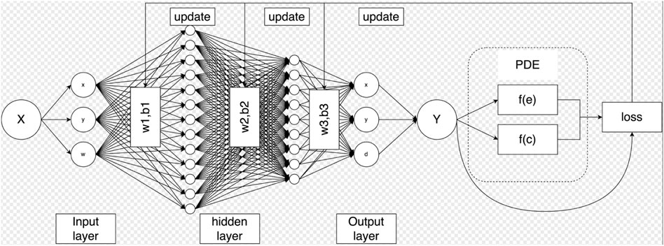
FIGURE 2. Schematic representation of the proposed physics informed neural network. X represents the input of the neural network, Y represents the output of the neural network, f(e) represents the elastic strain energy, and f(c) represents the fracture energy. For training, we have used the ADAM optimizer followed by L-BFGS.

4 Numerical examples

4.1 One dimensional cracked elastic bar

We are analyzing a bar with a crack located at the center (x = 0) and it is fixed at both ends (x = −1, x = 1). This bar is subjected to a sinusoidal load. The geometric setup is shown in Figure 3. For a given material, we take into account the elastic property E, material strength σ_c, and fracture energy G_c as the primary parameters. This implies that for the commonly used quadratic degradation function in Eq. 7, the length scale l₀ is not a separate variable and is valued as $l_0=27G_{c}E/256{\sigma }_c^2$. We choose the following parameters for this model: σ_c = 0.15MPa, G_c = 2.7N/m, E = 1MPa, and l₀ = l_p = 12.5 μm. The mesh size h in the vicinity of the crack is h = l₀. The crack at center is imposed by the following initial strain-history function:

$H\left(x,0\right)=\left\{\begin{array}{ccc}\hfill 1000\hfill & \hfill \mathrm{i}\mathrm{f}\hfill & \hfill d\left(x\right)\le l_0\hfill \\ \hfill 0\hfill & \hfill \mathrm{i}\mathrm{f}\hfill & \hfill d\left(x\right)>l_0\hfill \end{array}\right.(27)$

where l₀ is the length scale parameter. The displacement field satisfies the Dirichlet boundary conditions, i.e.,

$u\left(1\right)=u\left(-1\right)=0(28)$

The analytical solution of the displacement field Schillinger et al. [29] is discontinuous and is given by the following equation:

$u_{ex}=\left\{\begin{array}{ccc}\hfill \frac{1}{{\pi }^2}\sin \left(\pi x\right)-\frac{1+x}{\pi }\hfill & \hfill \mathrm{i}\mathrm{f}\hfill & \hfill x<0\hfill \\ \hfill \frac{1}{{\pi }^2}\sin \left(\pi x\right)+\frac{1-x}{\pi }\hfill & \hfill \mathrm{i}\mathrm{f}\hfill & \hfill x\ge 0\hfill \end{array}\right.(29)$

and phase field solutions is,

$d_{ex}=\exp \left(\frac{-|x-a|}{l_0}\right)(30)$

where the crack is located at ‘a’. For this problem, the configurations of the neural network are: three hidden layers and a subsequent linear layer, we use adaptive tanh activation function in the hidden layer, while for the last layer, we adopt a linear activation function. The optimization is first performed using the Adam optimizer, and then the L-BFGS optimizer is used, where the learning rate of the L-BFGS optimizer is α = 0.001. The one-dimensional elastic bar is divided into three regions: l_c: [−1, − 2L₀], c: [−2L₀, 2L₀], r_c: [2L₀, 1], where lc and rc respectively represent the left and right crack regions, and c is the crack region. To ensure that the output of the neural network fully satisfies the boundary conditions of Dirichlet, we set:

$u=\left[\left(x+1\right)\left(x-1\right)\right]u_{\theta }(31)$

where u_θ is the displacement field obtained as the output of the neural network. To optimize the proposed Physics-Informed Neural Network (PINN), we minimize the total variational energy of the system, which is defined in Eq. 20. To evaluate the precision of the results derived using this approach, we adopt two metrics: the relative error $L_2^{\mathit{rel}}$ and the root mean square error (RMSE).

FIGURE 3

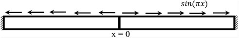
FIGURE 3. Geometrical setup of a one-dimensional elastic bar with crack.

Next, we study the effect of the proposed degradation function on the model. First, for the proposed degradation function, it can decouple between the length of the coupling field, l₀, and the physical length, l_p. By setting different q values, we can make l₀ multiple times larger than l_p. For instance, l₀ = 100l_p when q = 1.00155. Figure 4 shows the simulation results in cases of l₀ = l_p = 0.0125, 1/10L₀ = l_p = 0.00125 and 1/100L₀ = l_p = 0.000125. To ensure an impartial evaluation, both methods were tested using the same neural network architecture and the number of integral points. The results from the proposed method were then compared to those obtained from the AT2-based PINN approach. Figures 4A,B show the displacement field u and phase field d obtained using l_p = 0.0125. Visually, the obtained results overlap with the analytical solutions obtained using formulas Eqs. 29, 30. To quantify the accuracy of the proposed PINN method, relative errors and RMSEs corresponding to u and d are calculated. For u and d, the observed relative errors are 3.32% and 2.77%. In terms of the model size, 800 Gaussian points are involved. Corresponding to l_p = 0.00125 for u and d, relative prediction errors of 2.46% and 1.01%. Relative errors of u and d in case of l_p = 0.000125 of 20.56% and 48.28%. Note that the difference in Figures 4E,F is actually due to a lack of resolution at the material length scale. Therefore increasing the integration points appropriately and adjusting the number of training iterations may narrow the difference. The results shown in Figures 4E,F are not perfect. However, as the linear elastic fracture mechanics must meet the constraint of the phase-field process on a small scale zones, the constraint of the phase-field process on a small scale zones also applies to the proposed modeling method. Nevertheless, the phase field length scale can be selected independent of the inherent material process zone length scale, provided that the material processing zone length scale is sufficiently refined.

FIGURE 4

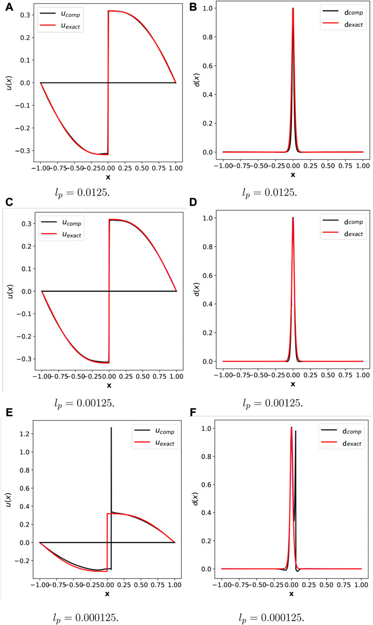
FIGURE 4. 1D elastic bar with crack using variation energy based PINN. Left column compares the exact displacement u_exact and the computed displacement u_comp. The right column compares the exact phase field d_exact and the computed phase field d_comp. (A) l_p = 0.0125, (B) l_p = 0.0125, (C) l_p = 0.00125, (D) l_p = 0.00125, (E) l_p = 0.000125, (F) l_p = 0.000125.

4.2 Single-edge notched plate subjected to tension

In this case, we take into consideration a unit square plate with a horizontal crack running from the midpoint of the left outer edge to the center of the plate. The problem’s geometry and boundary conditions are illustrated in Figure 5. The plate material has a tensile strength of σ_c = 2.54MPa, a fracture energy of G_c = 2.7N/m, a Young’s modulus of E = 282.69MPa, and a phase field length scale of l₀ = l_p = 12.5 μm. The mesh size, h, near the crack is h = l₀/4. The constant displacement increment applied during the computation is δv = 10⁻³mm. The crack path for the single-edge notched plate under tension was obtained using a fully connected neural network with three hidden layers, each of which has 50 neurons. The activation function for the first two layers adopt the tanh function, and for the last layer adopt the linear function. The initial crack was determined using the strain history functional described in Eq. 24. The boundary conditions imposed were Dirichlet boundary conditions.

$u\left(0,y\right)=v\left(x,0\right)=0,v\left(x,1\right)=\mathrm{\Delta }v(32)$

where u and v are the solutions of the elastic field along the x and y-axes, respectively. To satisfy the Dirichlet boundary conditions, the neural network outputs for the elastic field are modified as:

$u=\left[x\left(1-x\right)\right]\widehat{u}(33)$

$v=\left[y\left(y-1\right)\right]\widehat{v}+y\mathrm{\Delta }v(34)$

where $\widehat{u}$ and $\widehat{v}$ are obtained from the neural network. Figure 6 illustrates the crack propagation process in case of l_p = l₀ = 0.0125 mm. The result is very close to that of Goswami et al. [20].

FIGURE 5

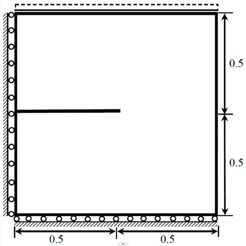
FIGURE 5. Geometrical setup and boundary conditions of the single-edge notched plate.

FIGURE 6

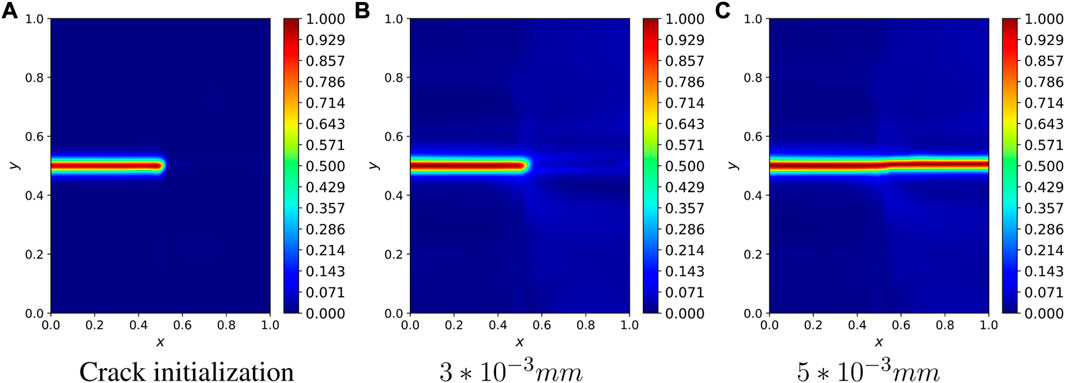
FIGURE 6. Phase field image of the single-edge notched plate at l₀ = l_p (A) Crack initialization, (B) 3 * 10⁻³ mm, (C) 5 * 10⁻³ mm.

As in the previous case, we first study the effect of the proposed degradation function on different physical length scale, l_p for the same size model. The ratio between l₀ and l_p is varied by setting different values of q. Figure 7 shows the simulation results for the cases l₀ = l_p = 0.0125mm, l₀ = 4l_p = 0.05 mm and l₀ = 10l_p = 0.125 mm. In the above simulation, we observe that when the length of the phase field increases, the number of required Gaussian integration points decreases considerably, when l₀ = l_p = 0.0125mm, the number of required integration points is: 20*20*16 (20 represents the mesh of elements and 16 represents the number of required integration points per element), when l₀ = 4l_p = 0.05mm, the number of required integration points is: 15*15*16, When l₀ = 10l_p = 0.125mm, the number of integration points required is: 12*12*16, and the same simulation speed is also increased. Therefore, assuming that the model is enlarged and the l_p is unchanged, does it mean that we can simulate the harsh conditions in the large-scale model where the physical length scale, l_p has to be small. We will therefore next investigate increasing the size of the model while keeping the length scale of the physical process zone constant. The previous example in Section 4.1 shows that decoupling the physical length scale from the phase field length is achievable albeit with limitations. The proposed degradation function allows to solve large-scale problem with much less computational cost. Suppose we multiply the length of the model edge by a factor of 4 and 10. In the meanwhile, the value of q is modified so that l₀ = 4l_p and l₀ = 10l_p. The value of σ_c remains constant all the time. The proposed degradation function allows to increase the size of l₀ and decrease the mesh, $\frac{1}{h}$ (which is closely related to the size of l₀, usually h = l₀/4), while keeping the physical length scale l_p constant. Simulation results for l₀ = 4l_p and l₀ = 10l_p are shown in figures Figure 8 and Figure 9. With the classical degradation function, if we want to increase the model by a factor of 10, we would need to add more integration points, whereas with the proposed degradation function, we can keep the number of integration points almost unchanged while increasing the model size by a factor of 10. We observe that the crack path shape is accurately captured by the larger length scale of the phase field. This adjustment to the phase field model formulation, therefore, allows for an increased sample size without the need for a significant increase in the computational volume of the length scale of the material processing zone.

FIGURE 7

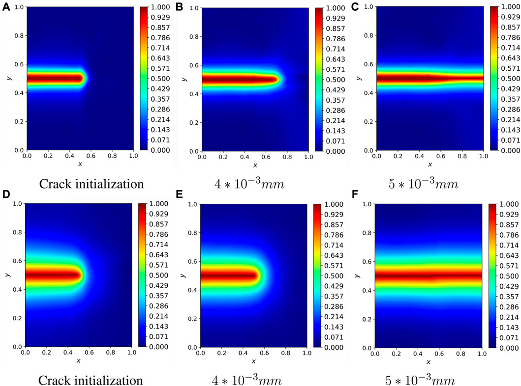
FIGURE 7. Phase field images of single-edge notched plates with the same model size and different l₀ values. The upper half: l₀ = 4l_p=0.05. The low half: l₀ = 10l_p = 0.125. (A) Crack initialization, (B) 4 ∗ 10⁻³ mm, (C) 5 ∗ 10⁻³ mm, (D) Crack initialization, (E) 4 ∗ 10⁻³ mm, (F) 5 ∗ 10⁻³ mm.

FIGURE 8

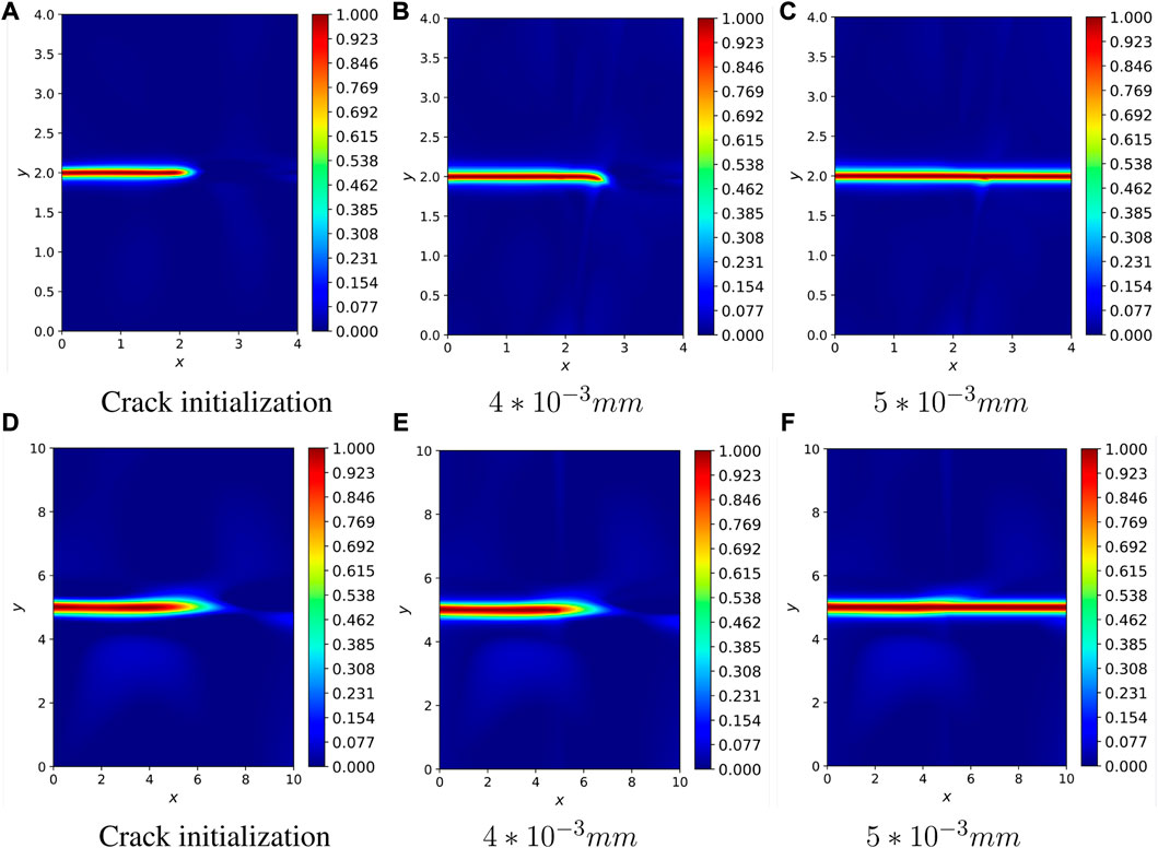
FIGURE 8. Phase field images of single-edge notched plates with 4 and 10 times of model enlargement while maintaining the peak stress unchanged. The upper half: l₀ = 4l_p. The low half: l₀ = 10l_p, (A) Crack initialization, (B) 4 ∗ 10⁻³ mm, (C) 5 ∗ 10⁻³ mm, (D) Crack initialization, (E) 4 ∗ 10⁻³ mm, (F) 5 ∗ 10⁻³ mm.

FIGURE 9

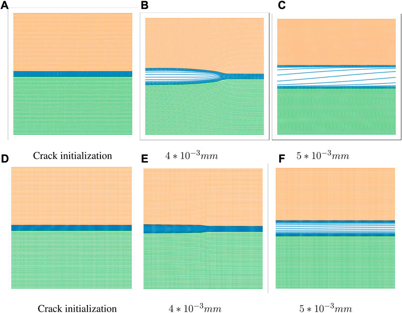
FIGURE 9. Scatter plots of single-sided notched plates with 4 and 10 times of model enlargement while maintaining the peak stress unchanged. The upper half: l₀ = 4L_p. The low half: l₀ = 10l_p, (A) Crack initialization, (B) 4 ∗ 10⁻³ mm, (C) 5 ∗ 10⁻³ mm, (D) Crack initialization, (E) 4 ∗ 10⁻³ mm, (F) 5 ∗ 10⁻³ mm.

4.3 Symmetrically double-edge notched plate sujected to tension

To verify the proposed method, we add another case, in which a double-edge notched plate subjected to a tensile load (see Figure 10) is considered. The material parameters are σ_c = 2.54Mpa, G_c = 2.7*10N/m, E = 282.69Mpa, and l₀ = l_p = 12.5 μm.

FIGURE 10

FIGURE 10. Geometrical setup and boundary conditions of the symmetrically double-edge notched plate.

To determine the crack path, we employed a fully connected neural network that includes four hidden layers, each of which has 50 neurons. The first three layers use the tanh activation function, while the final layer uses the linear activation. Both of cracks were initiated using the strain history functional, and the Dirichlet boundary conditions are specified:

$u\left(x,0\right)=v\left(x,0\right)=0,v\left(x,1\right)=\mathrm{\Delta }v(35)$

The solution for the elastic field along the x and y-axes are represented by u and v, respectively. In order to determine the crack path, a constant displacement increment of δu = 0.5∗10⁻⁴ mm has been applied. The output from the neural network for the elastic field is adjusted to conform with the Dirichlet boundary conditions:

$u=y\widehat{u}(36)$

$v=\left[y\left(y-1\right)\right]\widehat{v}+y\mathrm{\Delta }v(37)$

where $\widehat{u}$ and $\widehat{v}$ are obtained from the neural network. The value of q is set to be 200. Figure 11 show the predicted crack propagation as a function of the tensile displacement. The predicted results are compared with the results in Goswami et al. [20], and our findings are highly consistent with the results reported in the literature.

FIGURE 11

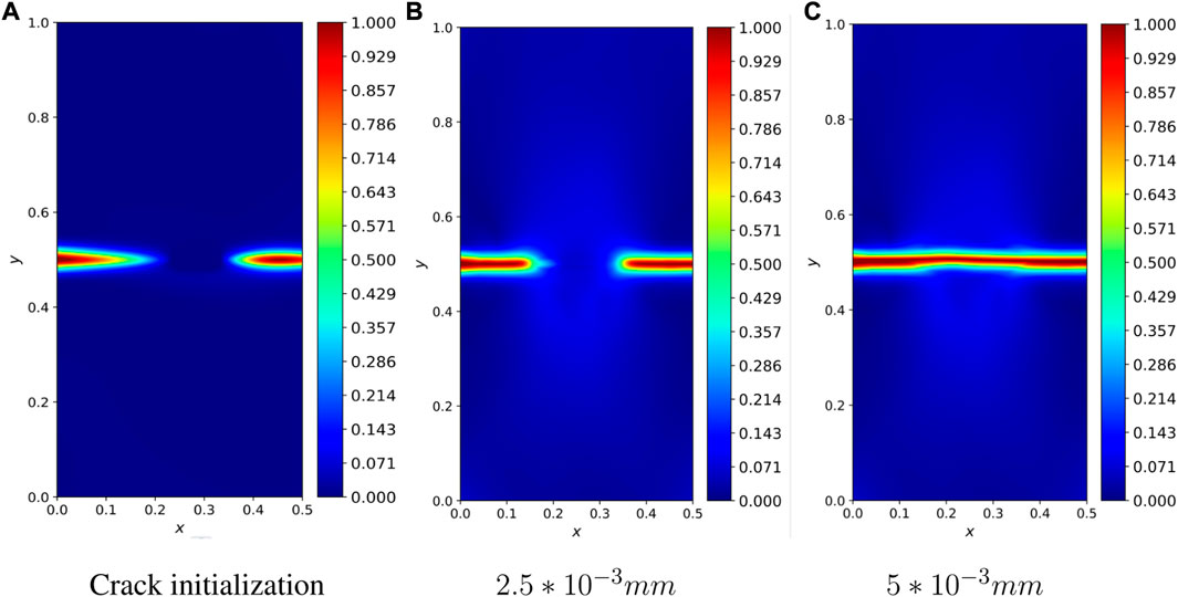
FIGURE 11. Phase field images of Symmetric double notched plates at l₀ = l_p, (A) Crack initialization, (B) 2.5 * 10⁻³ mm, (C) 5 * 10⁻³ mm.

We multiply the lengths of the model edges by factors of 4 and 10, and modify the value of q so that l₀ = 4l_p and l₀ = 10l_p. The value of σ_c is kept constant. The simulation results are shown in Figure 12 and Figure 13. Compared to the classical degradation function, there is no substantial increase in the running time when the model is expanded by a factor of 10 (mainly a small increase in the number of neural network iterations). We can find that with by introducing the length-scale separating degradation function to the PINN-based phase field model, maintaining a given mesh density sufficient to solve a larger scale model.

FIGURE 12

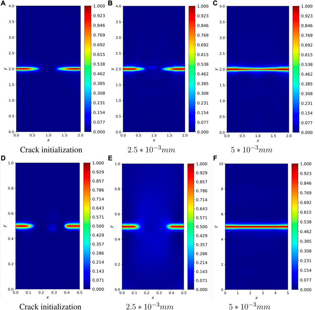
FIGURE 12. Phase field images of Symmetric double notched plates with 4 and 10 times of model enlargement while maintaining the peak stress unchanged. The upper half: l₀ = 4l_p. The low half: l₀ = 10l_p, (A) Crack initialization, (B) 2.5 * 10⁻³ mm, (C) 5 * 10⁻³ mm, (D) Crack initialization, (E) 2.5 * 10⁻³ mm, (F) 5 * 10⁻³ mm.

FIGURE 13

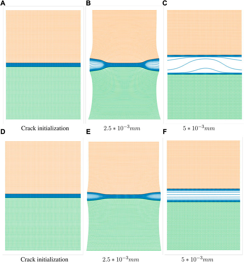
FIGURE 13. Scatter plots of Symmetric double notched plates with 4 and 10 times of model enlargement while maintaining the peak stress unchanged. The upper half: l₀ = 4l_p. The low half: l₀ = 10l_p, (A) Crack initialization, (B) 2.5 * 10⁻³ mm, (C) 5 * 10⁻³ mm, (D) Crack initialization, (E) 2.5 * 10⁻³ mm, (F) 5 * 10⁻³ mm.

5 Conclusion and outlook

In this paper, we enhanced PINN-based phase field method (Goswami et al. [20], Goswami et al. [21]) with the degradation functions proposed by Lo et al. [9] in order to simulate fracture propagation in large structures. In conventional phase field method, the length scale of the phase field length scale is set to equate the physical length scale, which is very small compared to the structure size. Because a very refined mesh is needed to represent the diffuse fracture zone, it is impractical to apply PINN-based phase field method to large-scale models. To solve this problem, we introduce to PINN-based phase field simulation the degradation function that decouples the length scales of the phase field and the physical process zone. The merits and limitations of the modified phase field approach are discussed through several numerical examples. The proposed method combines the advantages of data driven and mechanism based computational approaches and improved its efficiency in fracture simulation. Although these examples are only for 2D problems, it is expected that the method could be applied to 3D situations without issue. In the future, we will investigate the uncertainty quantification of fractures with the present method. In addition, we will extend the present method to the hydraulic fracture problems.

Data availability statement

The original contributions presented in the study are included in the article/supplementary material, further inquiries can be directed to the corresponding author.

Author contributions

HL: Software, Methodology, Writing, Administration; PZ: Software, Writing; MZ: Methodology, Revision; PW: Methodology; YL: Methodology, Adminstration. All authors contributed to the article and approved the submitted version.

Funding

The authors appreciate the financial support from the National Natural Science Foundation of China (NSFC) under Grant Nos. 52274222 and 51904202.

Conflict of interest

Author PW was employed by Beijing Huituo Infinite Technology Co., Ltd.

The remaining authors declare that the research was conducted in the absence of any commercial or financial relationships that could be construed as a potential conflict of interest.

Publisher’s note

All claims expressed in this article are solely those of the authors and do not necessarily represent those of their affiliated organizations, or those of the publisher, the editors and the reviewers. Any product that may be evaluated in this article, or claim that may be made by its manufacturer, is not guaranteed or endorsed by the publisher.

References

1. Moës N, Dolbow J, Belytschko T. A finite element method for crack growth without remeshing. Int J Numer Methods Eng (1999) 46:131–50. doi:10.1002/(sici)1097-0207(19990910)46:1<131:aid-nme726>3.0.co;2-j

CrossRef Full Text | Google Scholar

2. Aliabadi MH. The boundary element method, volume 2: Applications in solids and structures, vol. 2. New York, NY, USA: John Wiley & Sons (2002).

Google Scholar

3. Pereira K, Wahab MA. Fretting fatigue lifetime estimation using a cyclic cohesive zone model. Tribology Int (2020) 141:105899. doi:10.1016/j.triboint.2019.105899

CrossRef Full Text | Google Scholar

4. Pereira K, Bhatti N, Wahab MA. Prediction of fretting fatigue crack initiation location and direction using cohesive zone model. Tribology Int (2018) 127:245–54. doi:10.1016/j.triboint.2018.05.038

CrossRef Full Text | Google Scholar

5. Zi G, Belytschko T. New crack-tip elements for XFEM and applications to cohesive cracks. Int J Numer Methods Eng (2003) 57:2221–40. doi:10.1002/nme.849

CrossRef Full Text | Google Scholar

6. Ha YD, Bobaru F. Studies of dynamic crack propagation and crack branching with peridynamics. Int J Fracture (2010) 162:229–44. doi:10.1007/s10704-010-9442-4

CrossRef Full Text | Google Scholar

7. Bourdin B, Francfort GA, Marigo J-J. Numerical experiments in revisited brittle fracture. J Mech Phys Sol (2000) 48:797–826. doi:10.1016/s0022-5096(99)00028-9

CrossRef Full Text | Google Scholar

8. Wu J.Y., Nguyen V.P. (2018). A length scale insensitive phase-field damage model for brittle fracture. 392 Journal of the Mechanics and Physics of Solids. 119, 20-42.

CrossRef Full Text | Google Scholar

9. Lo Y-S, Hughes TJ, Landis CM. Phase-field fracture modeling for large structures. J Mech Phys Sol (2023) 171:105118. doi:10.1016/j.jmps.2022.105118

CrossRef Full Text | Google Scholar

10. Li Z, Liu F, Yang W, Peng S, Zhou J. A survey of convolutional neural networks: Analysis, applications, and prospects. IEEE Trans Neural networks Learn Syst (2021) 33:6999–7019. doi:10.1109/tnnls.2021.3084827

CrossRef Full Text | Google Scholar

11. Glorot X, Bengio Y. Understanding the difficulty of training deep feedforward neural networks. In: Proceedings of the thirteenth international conference on artificial intelligence and statistics (JMLR Workshop and Conference Proceedings) (2010). p. 249–56.

Google Scholar

12. Karumuri S, Tripathy R, Bilionis I, Panchal J. Simulator-free solution of high-dimensional stochastic elliptic partial differential equations using deep neural networks. J Comput Phys (2020) 404:109120. doi:10.1016/j.jcp.2019.109120

CrossRef Full Text | Google Scholar

13. Simonyan K, Zisserman A. Very deep convolutional networks for large-scale image recognition (2014). arXiv preprint arXiv:1409.1556.

Google Scholar

14. Albawi S, Mohammed TA, Al-Zawi S. Understanding of a convolutional neural network. In: 2017 international conference on engineering and technology (ICET). Antalya, Turkey: IEEE (2017). p. 1–6. doi:10.1109/ICEngTechnol.2017.8308186

CrossRef Full Text | Google Scholar

15. Raissi M, Perdikaris P, Karniadakis GE. Physics-informed neural networks: A deep learning framework for solving forward and inverse problems involving nonlinear partial differential equations. J Comput Phys (2019) 378:686–707. doi:10.1016/j.jcp.2018.10.045

CrossRef Full Text | Google Scholar

16. Raissi M. Deep hidden physics models: Deep learning of nonlinear partial differential equations. J Machine Learn Res (2018) 19:932–55.

Google Scholar

17. Raissi M, Yazdani A, Karniadakis GE. Hidden fluid mechanics: A Navier-Stokes informed deep learning framework for assimilating flow visualization data (2018). arXiv preprint arXiv:1808.04327.

Google Scholar

18. Zhu Y, Zabaras N, Koutsourelakis P-S, Perdikaris P. Physics-constrained deep learning for high-dimensional surrogate modeling and uncertainty quantification without labeled data. J Comput Phys (2019) 394:56–81. doi:10.1016/j.jcp.2019.05.024

CrossRef Full Text | Google Scholar

19. Geneva N, Zabaras N. Modeling the dynamics of PDE systems with physics-constrained deep auto-regressive networks. J Comput Phys (2020) 403:109056. doi:10.1016/j.jcp.2019.109056

CrossRef Full Text | Google Scholar

20. Goswami S, Anitescu C, Chakraborty S, Rabczuk T. Transfer learning enhanced physics informed neural network for phase-field modeling of fracture. Theor Appl Fracture Mech (2020) 106:102447. doi:10.1016/j.tafmec.2019.102447

CrossRef Full Text | Google Scholar

21. Goswami S, Anitescu C, Rabczuk T. Adaptive phase field analysis with dual hierarchical meshes for brittle fracture. Eng Fracture Mech (2019) 218:106608. doi:10.1016/j.engfracmech.2019.106608

CrossRef Full Text | Google Scholar

22. Francfort GA, Marigo JJ. Revisiting brittle fracture as an energy minimization problem. J Mech Phys Sol (1998) 46:1319–42. doi:10.1016/s0022-5096(98)00034-9

CrossRef Full Text | Google Scholar

23. Lie J, Lysaker M, Tai X-C. A binary level set model and some applications to mumford-shah image segmentation. IEEE Trans image Process (2006) 15:1171–81. doi:10.1109/tip.2005.863956

PubMed Abstract | CrossRef Full Text | Google Scholar

24. Amor H, Marigo JJ, Maurini C. Regularized formulation of the variational brittle fracture with unilateral contact: Numerical experiments. J Mech Phys Sol (2009) 57:1209–29. doi:10.1016/j.jmps.2009.04.011

CrossRef Full Text | Google Scholar

25. Miehe C, Welschinger F, Hofacker M. Thermodynamically consistent phase-field models of fracture: Variational principles and multi-field fe implementations. Int J Numer Methods Eng (2010) 83:1273–311. doi:10.1002/nme.2861

CrossRef Full Text | Google Scholar

26. Miehe C, Hofacker M, Welschinger F. A phase field model for rate-independent crack propagation: Robust algorithmic implementation based on operator splits. Comput Methods Appl Mech Eng (2010) 199:2765–78. doi:10.1016/j.cma.2010.04.011

CrossRef Full Text | Google Scholar

27. LeCun Y, Bengio Y, Hinton G. Deep learning. Nature (2015) 521:436–44. doi:10.1038/nature14539

PubMed Abstract | CrossRef Full Text | Google Scholar

28. Borden MJ, Verhoosel CV, Scott MA, Hughes TJ, Landis CM. A phase-field description of dynamic brittle fracture. Comput Methods Appl Mech Eng (2012) 217:77–95. doi:10.1016/j.cma.2012.01.008

CrossRef Full Text | Google Scholar

29. Schillinger D, Borden MJ, Stolarski HK. Isogeometric collocation for phase-field fracture models. Comput Methods Appl Mech Eng (2015) 284:583–610. doi:10.1016/j.cma.2014.09.032

CrossRef Full Text | Google Scholar