
94% of researchers rate our articles as excellent or good
Learn more about the work of our research integrity team to safeguard the quality of each article we publish.
Find out more
ORIGINAL RESEARCH article
Front. Phys., 27 September 2023
Sec. Medical Physics and Imaging
Volume 11 - 2023 | https://doi.org/10.3389/fphy.2023.1124980
This article is part of the Research TopicNovel MRI BiomarkersView all 5 articles
 Christoph Zöllner1*
 Sophia Kronthaler1
 Kilian Weiss2
 Christof Boehm1
 Jonathan Stelter1Jürgen Rahmer3
 Peter Börnert3Johannes M. Peeters4Daniela Junker1
 Dimitrios C. Karampinos1
Purpose: Multi-echo Stack-of-stars (SoS) radial k-space trajectories with golden angle ordering are becoming popular for free-breathing abdominal Dixon imaging and proton density fat fraction (PDFF) mapping. Gradient chain imperfections including eddy currents and system delays are known to affect the image quality of radial imaging and to confound the estimation of PDFF mapping. This work proposes a retrospective trajectory correction method based on a simple gradient modulation transfer function (GMTF) measurement to predict and correct gradient chain induced k-space trajectory errors.
Methods: The GMTF was measured using the standard hardware of a 3 Tesla scanner on a phantom using the thin slice method and was applied to a 3D radial SoS Dixon imaging sequence. The impact of the GMTF-based correction on image reconstruction and PDFF quantification was investigated using numerical simulations and validated on experimental phantom data as well as on in vivo leg and liver data of healthy volunteers.
Results: Correcting the k-space trajectories with the measured GMTF during image reconstruction reduced PDFF quantification errors for phantom and in vivo acquisitions. A Bland-Altman comparison of the measured PDFF phantom and reference data confirmed that the GMTF correction narrowed down the limits of agreement (LoA) from 1.3%
Conclusion: The proposed GMTF-based k-space trajectory correction is a fast alternative method for avoiding PDFF quantitation errors caused by gradient-system induced k-space trajectory errors in 3D radial multi-echo gradient-echo acquisitions.
Chemical shift encoding based water-fat separation techniques have been emerging for efficient fat suppression and fat quantification across organs [1, 2]. By acquiring the MR signal at different echo times, the so-called Dixon techniques encode water and fat in the time domain. The water and fat images can be estimated by fitting a signal model that accounts for confounding factors such as the T1 bias [3, 4], the T2* decay [5–7], the spectral complexity of fat [8], the noise bias [3] and eddy currents [9, 10] in a way that consequently a quantitative proton-density fat fraction (PDFF) map can be calculated. In abdominal MRI, the liver PDFF is an established biomarker for assessment of hepatic steatosis [11, 12] and is being used also beyond routine diagnostic imaging in lifestyle intervention studies [13].
While abdominal PDFF mapping is performed conventionally with Cartesian k-space trajectories [6–10], abdominal Dixon acquisitions can suffer from high motion sensitivity. They are therefore typically performed during a breath-hold, which limits achievable volumetric coverage, spatial resolution, or signal-to-noise ratio. This complicates the application of Dixon methods in subjects unable to suspend respiration, such as sick, elderly, or pediatric patients. Radial acquisitions are more robust to motion than Cartesian acquisitions, since they sample the k-space center continuously [14]. Radial stack-of-stars acquisitions enable the continuous sampling of the k-space center in 3D imaging and have been combined with Dixon imaging [15]. There have been multiple recent works proposing free-breathing motion-averaged or motion-resolved multi-echo radial SoS acquisitions to quantify PDFF in a free-breathing mode [16–21].
Due to varying readout directions, radial acquisitions are more sensitive to phase errors induced by gradient chain imperfections than their Cartesian counterpart. The gradient chain connects the input of the three physical x-, y- and z-waveforms to the gradient fields in the scanner bore and consists of pre-emphasis for eddy current compensation, the three gradient amplifiers, and respective gradient coils. Gradient system imperfections, more precisely eddy currents, gradient system delays and vibrations, or an inadequate pre-emphasis, cause k-space trajectory errors in radial acquisitions, resulting in deteriorated image quality [22–24]. It is already known from Cartesian acquisitions that phase errors induced by eddy currents cause a bias in abdominal fat quantification when using complex-based [25] chemical shift encoding based water–fat separation techniques [26–28]. Thus, when radial k-space trajectories are used for chemical shift encoding based water–fat separation, gradient chain imperfections are expected to affect the image quality of the multi-echo images and to induce bias in the PDFF quantification.
Eddy current correction techniques either use specialized NMR field probes to measure the gradients directly [29–31], perform separate calibration scans [32–35] or estimate the errors directly from the measured raw data without any additional calibration scans [36–39]. It had also been shown that eddy currents can be corrected by measuring the transfer function that describes the gradient system characteristics. In the context of radial water–fat imaging, most previous methods relied on the acquisition of calibration lines for each gradient axis with opposite polarity to determine the gradient timing errors [15–21]. However, the acquisition of such calibration lines prolongs the acquisition time and must be repeated for each scan. It has been also demonstrated that a data-driven correction can estimate k-space shifts from radial raw data [40] and be applied in the context of PDFF mapping using a radial SoS acquisition [41]. A more general approach to correcting the errors induced by the gradient system imperfections can be achieved with the use of a gradient impulse response function (GIRF) [32, 42] or its Fourier transform, the gradient modulation transfer function (GMTF), under the assumption that the gradient system behaves linearly and time invariant. The GMTF measurement enables full characterization of the scanner gradient system chain in frequency space. Once the GMTF is known, arbitrary gradient waveforms from any pulse sequence can be corrected. The GMTF itself can be measured either with special NMR field probes [29, 30, 42, 43], or using the thin slice method in simple phantoms [32, 33], [44–46]. It has been shown that a GMTF-based trajectory correction for gradient imperfections improves image quality in non-Cartesian spiral acquisitions [32, 47]. However, it has not been applied to abdominal radial SoS Dixon imaging yet.
The purpose of this work is to propose a correction for gradient chain imperfections in abdominal radial SoS-based PDFF mapping based on a GMTF measurement, using the thin slice method without the need of any additional hardware. The impact of the GMTF correction on the PDFF quantification is investigated in simulations and validated in phantom and in vivo scans.
Each linear time invariant system can be fully characterized by its impulse response function, which describes the time-domain response of the system to an idealized point impulse [48]. The Fourier transform of this impulse response function yields the modulation transfer function. For most applications the MRI gradient chain can be treated as a linear time invariant system and as such it can be described by the GIRF
Written in the frequency domain the convolution becomes a multiplication:
where
The measurement of the GMTF/GIRF itself is based on a thin slice method by Rahmer et al [45] which was simplified by Kronthaler et al [50] for the application in radial imaging. The thin slice method is based on the work by Duyn et al [33], where it was shown that the excitation of a thin slice, generating a 1D virtual probe, is sufficient to measure the behavior of the gradient system without any additional hardware. Applying a test gradient along the direction of the slice selection of the 1D probe allows the measurement of the response to the test gradient.
Neglecting B0 drift, through-slice dephasing and assuming homogeneous fields in y and z direction, the following signal model describes such a 1D probe GIRF measurement in the x-direction, with the distance
i.e.,
The evolution of
The spatial 0th order term is related to temporal variations in the B0 field and the first order terms to temporal variations of the field gradients. k1, k2 and k3 can be identified as the k-space coordinates kx, ky and kz. A 1D measurement in the x-direction corresponds to
To get rid of confounding signal contributions (
In order to measure the spatial variation of the system response, several slices at different off-center locations are excited. The measured phase is then expanded into polynomials up to the second order [46] given by
The real gradient applied along the x-axis can be then calculated using the first-order component of the fitted phase.
The GMTF is calculated in the Fourier domain as follows [42, 52].
Rahmer et al. extended the GMTF measurement to 3D by adding a phase encoding gradient. They reported that a 1D GMTF measurement is sufficient since second order components were often negligible. Thus, a simplified measurement technique was used in this work to estimate the first order response by measuring the signal from 4 parallel off-center slices per gradient axis [50].
A spherical phantom (diameter 166 mm, volume 2 liters), containing CuSO4-doped water (relaxation time values at 3 Tesla: T1 ≈ 280 ms and a T2 ≈ 240 ms) was used to measure the GMTF. Four slices of 1.5 mm thickness were excited with an excitation pulse with length 1.6 ms, a maximum amplitude of 5.45 μT and a flip angle of 45°. The four slices were located at distances of −26.25 mm, −8.75 mm, 8.75 mm, and 26.25 mm from the iso-center. A chirp waveform was chosen as the input test gradient with a frequency range of 0.1–10.0 kHz with an acquisition window of 80 ms (Figure 1). The measurement was performed separately along each gradient axis.
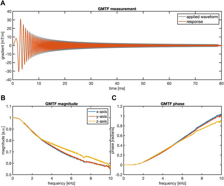
FIGURE 1. GMTF measurement results. (A) The applied chirp gradient waveform and its measured response in the time domain which are used to calculate the magnitude (B) and the phase (C) of the GMTF for each gradient direction. In (A) only the response of the x-direction gradient is shown for the sake of clarity.
The performance of the GMTF correction method was demonstrated for PDFF mapping using a radial SoS acquisition employing a multi-echo readout (Figure 2A) on a 3 T system (Elition X, Philips Healthcare, Best, the Netherlands). The spokes in the kx-ky-plane were acquired in a pseudo golden angle ordering [53], which provides a homogeneous distribution of the acquired spokes in k-space while still relying on a golden angle increment of 111.25°. Radial spokes with the same azimuthal angle were acquired for all kz increments prior to azimuthal angle rotation. The Cartesian kz-dimension was aligned with the B0-direction. SENSE acceleration was also applied in the z-dimension for scan time reduction [54].
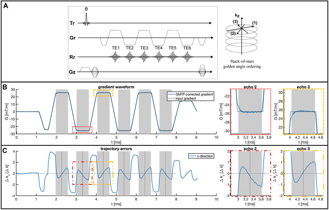
FIGURE 2. GMTF-based trajectory error estimation. (A) The six-echo gradient-echo radial stack-of-stars sequence with pseudo golden angle ordering used for PDFF mapping. (B) GMTF correction of the input gradient waveform for one TR. The gray areas mark the acquisition windows of the single echoes. Zoomed-in views of the second and third echo are shown on the right highlighting the gradient chain induced deviations at the beginning of each echo readout. (C) Corresponding corrected trajectory errors for the x-encoding direction for one TR, based on the GMTF-corrected gradient waveform. The echo times are marked by the vertical black lines. Zoomed in views of echo 2 and 3 are shown on the right in (B) and (C).
The GMTF correction method was implemented as a retrospective correction of the trajectory during the image reconstruction process [43, 47, 50, 52]. Before applying the GMTF correction to any logical gradients, the gradients were transformed to the physical gradient system by linear transformations. After applying the GMTF, the inverse transformation was used to calculate the corrected logical gradients. To obtain the exact k-space positions of the acquired data points, the real gradient waveform was predicted by convolving the input gradient waveform with the measured GIRF in the time domain. This convolution operation was performed as a multiplication of the Fourier-transformed input gradient waveform of a whole repetition time with the GMTF, thus providing the corrected gradient waveform of all six echoes (Figure 2B). Integration of this gradient waveform yielded the GMTF-corrected trajectory and a gridding-based non-Cartesian image reconstruction was performed subsequently. The data was gridded in the kx-ky-plane with the corresponding trajectories using a Kaiser-Bessel kernel of width 4 k-space sampling steps and a gridding oversampling factor of 1.25. The gridding operation, the Fourier transform in 3D and the SENSE unfolding in the third Cartesian-sampled z-dimension were performed using an image reconstruction toolbox (ReconFrame, Gyrotools, Switzerland). The same toolbox was also used to access all necessary information about the gradient objects for each sequence from the raw data to reconstruct the gradient waveform, which will be used during the GMTF correction.
An additional data-driven correction method for gradient delays was implemented to compare it with the performance of the proposed GMTF correction. The intrinsic design of the SoS trajectory allows for a data-driven correction of gradient delay induced k-space shifts. Spokes of approximately opposite readout polarity within the kx-ky-plane were used to estimate these k-space shifts [24, 40]. Given that a constant shift in k-space can be represented as a linear phase term in image space, according to the Fourier shift theorem, the k-space shift was determined by fitting the linear phase in image space [28]: Therefore, the signal of each spoke was correlated in image space with the signal of the corresponding spoke with opposite readout direction to estimate a linear phase offset. Following that, the estimated linear phase offset was applied to each spoke in image space. It must be noted that this spoke alignment method corrects the k-space signal by shifting the signal along the frequency encoding direction while not changing the k-space trajectory. The spoke alignment method can be thus simply performed prior to the gridding routine.
A simulation was performed to investigate the impact of gradient chain induced trajectory errors on PDFF quantification. Therefore, the correction of a six-echo gradient-echo acquisition in a water-only spherical numerical phantom was investigated. K-space data was simulated from a numerical water phantom via a NUFFT operation based on the GMTF-corrected trajectory to generate the reference data. Gradient-chain system errors were modeled by performing a NUFFT reconstruction of this data with the uncorrected ideal trajectory which does not account for any gradient imperfections. A reference reconstruction was performed with the GMTF-corrected trajectory and both reconstructed data sets were passed through a water–fat separation pipeline to generate PDFF maps. All NUFFT operations were performed via the NUFFT implementation from BART [55] and all sequence parameters and the trajectories were selected based on the water phantom measurements (for a detailed list of parameters, please refer to the subsection “Phantom measurements” below). A T2*- decay of 20 ms was assumed for the water signal during signal simulation. PDFF maps were obtained via a complex-based water–fat separation assuming a single T2* decay and the same multi-peak fat spectrum that is used for processing the measured phantom data. The water-fat separation problem was solved based on a variable-layer single-min-cut graph-cut algorithm [56]. The GMTF-corrected and uncorrected PDFF maps were compared qualitatively.
Two different phantoms were scanned to evaluate the performance of the GMTF correction. First, a simple water bottle phantom was scanned to replicate the simulation setup, using a 3D six-echo gradient-echo radial SoS sequence with pseudo golden angle ordering. The exact sequence parameters were TE = 1.40 ms/2.44 ms/3.47 ms/4.51 ms/5.55 ms/6.59 ms, TR = 10.40 ms, flip angle = 3°, in-plane resolution = 1.5 × 1.5 mm2, slice thickness = 3.0 mm, FOV = 450 × 450 × 159 mm3, 391 spokes, 300 samples per spoke, 53 slices, bandwidth = 1613 Hz/pixel, scan time of 5 min 13 s. Second, a PDFF phantom (Calimetrix, Madison, USA) containing 15 vials with different fat fractions ranging from 0% to 100% (PDFF reference values of the vials [%]: 0.1
Both phantom scans were reconstructed with the original k-space trajectory and the GMTF-corrected k-space trajectory. The PDFF phantom data was additionally corrected with the spoke alignment method for comparison. Subsequently, PDFF maps were calculated based on a complex-based water–fat separation with a variable-layer single-min-cut graph-cut algorithm. The magnitude discrimination approach was employed to minimize noise bias effects [3]. A peanut oil-based fat model was used to fit the signal of the phantom acquisitions to account for temperature shift and the fat composition of the PDFF phantom [57].
The PDFF reference values of the PDFF phantom were obtained with a Cartesian 6 echo time-interleaved multi-echo gradient echo sequence with two interleaves and monopolar gradient readouts [28] and the following parameters: TE1 = 1.24 ms, delta TE = 1.0 ms, TR = 7.8 ms, flip angle = 3.0°, resolution = 1.5 × 1.5 × 1.5 mm3, FOV = 190 × 190 × 190 mm3, bandwidth = 1415.2 Hz/pixel, scan duration = 3 min 38 s. The PDFF maps were calculated based on the scanner-reconstructed multi-echo images after phase-correction [28] with a complex-based water–fat separation with a variable-layer single-min-cut graph-cut algorithm.
The effect of the GMTF correction on PDFF quantification was also investigated in two in vivo anatomies, the liver and the upper thighs, as a reference for an anatomy without respiratory motion effects. Therefore both anatomies were scanned with the proposed SoS sequence and a low resolution Cartesian reference scan. The radial data was corrected with the proposed GMTF correction and the data-driven spoke alignment method respectively. PDFF maps of the corrected and uncorrected radial data sets were compared with the Cartesian reference PDFF maps qualitatively and via a ROI analysis for the liver data.
In vivo imaging of the liver and the upper thighs was performed on 11 healthy volunteers after approval by the institutional review board (Klinikum rechts der Isar, Technical University of Munich, Munich, Germany) and informed written consent by each subject. Imaging of the liver and the legs was performed axially with a 3D high resolution six-echo radial SoS sequence with pseudo golden angle ordering. The Cartesian z-dimension of the SoS trajectory was aligned with the patient’s feet–head axis.
The thighs were scanned with the radial SoS sequence using the following parameters: TE = 1.40 ms/2.43 ms/3.47 ms/4.51 ms/5.55 ms/6.59 ms, TR = 10.40 ms, flip angle = 3°, in-plane resolution = 1.5 × 1.5 mm2, slice thickness = 3.0 mm, FOV = 450 × 450 × 201 mm3, 391 spokes, 300 samples per spoke, 42 slices, bandwidth = 1634 Hz/pixel, scan time of 4 min 33 s, and SENSE acceleration factor of 1.6 in the Cartesian-sampled dimension.
Liver radial SoS imaging was performed using the following parameters: TE = 1.38 ms/2.41 ms/3.44 ms/4.48 ms/5.51 ms/6.55 ms, TR 10.0 ms, flip angle = 3°, in-plane resolution = 1.5 × 1.5 mm2, slice thickness = 3.0 mm, FOV = 450 × 450 × 201 mm3, 391 spokes, 300 samples per spoke, 42 slices, bandwidth = 1603 Hz/pixel, average scan time of 8 min 10 s, and SENSE acceleration factor of 1.6 in the Cartesian-sampled dimension. Breathing motion was compensated with a 1D-pencil beam navigator, placed in the feet–head direction within the liver dome and the diaphragm.
Both anatomies were scanned additionally with a low resolution 3D Cartesian Dixon sequence which is clinically used for PDFF assessment in the liver with the following parameters: TE = 0.92 ms/1.56 ms/2.21 ms/2.85 ms/3.50 ms/4.14 ms, TR = 10.0 ms, flip angle = 3°, in-plane resolution = 3.2 × 3.2 mm2, slice thickness = 6.0 mm, FOV = 450 × 450 × 198 mm3, scan time of 17 s (to fit in a single breath-hold for the liver acquisition). The Cartesian breath-hold scans were reconstructed and the water–fat separation steps were performed with the manufacturer’s online implementation.
The radial SoS scans were reconstructed offline without any trajectory correction, with the spoke alignment method and with the proposed GMTF correction method. PDFF maps were estimated with a complex-based water–fat separation with a variable-layer single-min-cut graph-cut algorithm. 9-peak fat models were used for the PDFF calculation of the liver [58] and leg [59] data sets.
Mean value and standard deviation of the corrected and uncorrected liver PDFF distributions were determined based on 4 ROIs (area = 4 cm2) placed at right, left, anterior and posterior positions of the liver [60].
Figure 1A shows the measured first order response to the chirp waveform test gradient for the x-gradient axis. Based on the response, the magnitude (Figure 1B) and phase (Figure 1C) of the GMTF
Figure 2B shows the result of the convolution of the gradient input waveform with the measured GMTF for the x-gradient direction. Large eddy current induced deviations of the GMTF-corrected waveform from the ideal input waveform were visible during the ramp-up process of each gradient and at the beginning of each echo readout. These errors were caused by short term eddy currents that decayed after the plateau of each gradient was reached. Long term eddy currents were not visible within one TR. Figure 2C shows the resulting trajectory errors for an exemplary radial spoke in the kx-direction, calculated based on the different sampling positions obtained with the GMTF-corrected gradient waveform and the uncorrected input waveform. The trajectory error varied during the echo readout: The largest errors were observed at the beginning and the end of each readout, where high spatial frequencies were sampled, reaching shifts of up to one k-space sampling step. Varying shifts were observed along the spoke and at the k-space center, while comparing odd and even echoes of the multi-echo acquisition.
The simulated impact of the trajectory errors propagating into the PDFF quantification is presented in Figure 3. Figure 3A shows the PDFF maps obtained from the simulated six-echo data of a water-only (PDFF = 0) sphere (Figure 3B) reconstructed with the uncorrected trajectory and the GMTF-corrected trajectory. The PDFF map obtained from the uncorrected data showed an inhomogeneous PDFF distribution. PDFF values reached values higher than 2% in the center of the sphere, while the values dropped significantly symmetrically towards the edge of the object to negative PDFF values as low as −8%. In contrast, the corrected PDFF map had a homogeneous distribution around zero as expected, showing only light reconstruction artifacts, stemming from the NUFFT operations. For example, ringing artifacts were visible at the edge of the phantom or the outer FOV. PDFF line profiles across the phantom are plotted in Figure 3C.
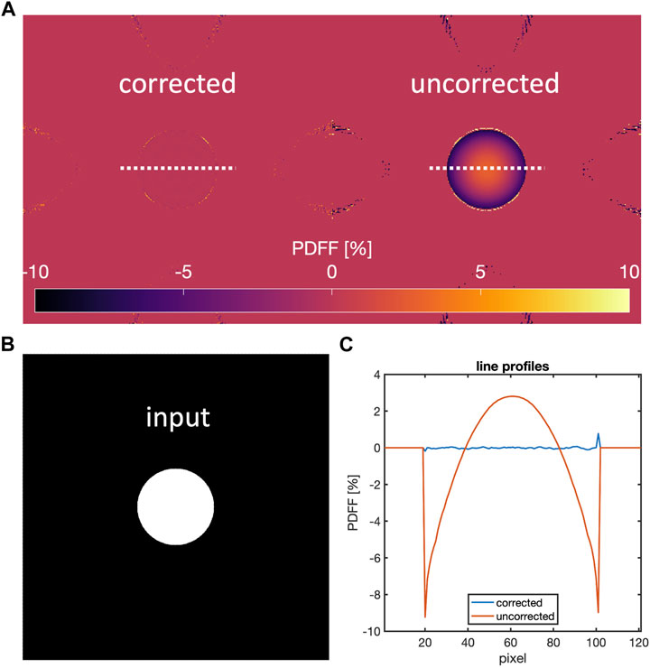
FIGURE 3. Numerical simulations of gradient-chain induced effects. (A) PDFF maps obtained from simulated six-echo data on a water sphere (B) generated with the GMTF-corrected trajectory and reconstructed with the corrected trajectory (upper left) and uncorrected trajectory (upper right). (C) shows PDFF line profiles along the dashed lines in (A). The trajectory errors cause PDFF estimation errors of up to 2% PDFF in the center and up to −8% PDFF at the edge of the numerical phantom.
Figure 4 shows PDFF maps of a water bottle phantom scan that were obtained from data reconstructed with the uncorrected trajectory and with the GMTF-corrected k-space trajectory. Using the uncorrected gradient waveform in the reconstruction process resulted in an inhomogeneous PDFF distribution with a positive PDFF bias towards the upper edge of the phantom and negative PDFF values around −5% PDFF at the bottom edge. In contrast, the reconstruction with the GMTF-corrected trajectory reduced the severe negative PDFF underestimations at the bottom edge, yielding a more homogeneous PDFF map than the uncorrected reconstruction.
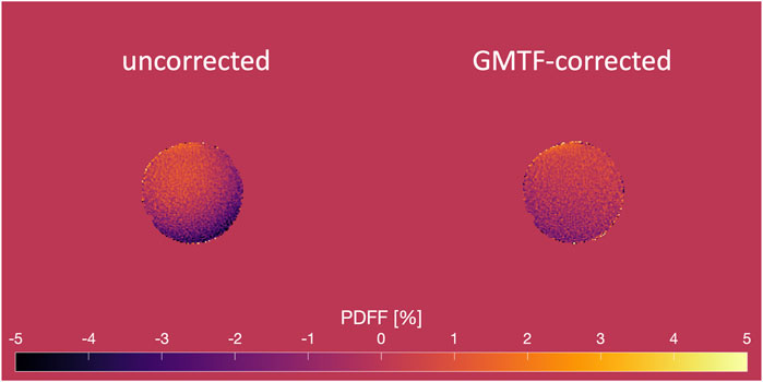
FIGURE 4. PDFF results of a water bottle phantom scan using a six-echo radial SoS acquisition. The PDFF map obtained from the uncorrected data (left) is inhomogeneous with a severe negative PDFF bias at the bottom right edge of the phantom. The GMTF correction results in a more homogeneous distribution and improves the negative PDFF bias at the bottom edge (right).
The results of the GMTF correction applied to the PDFF phantom scan are presented in Figure 5. Figure 5A displays the PDFF maps estimated with and without the GMTF correction applied during the image reconstruction step as well as PDFF maps from data corrected with the spoke alignment method. The visualization in the 0%–100% PDFF range revealed errors for the high PDFF fraction vials, especially the 82.5% and the 90.8% vial were over- or underestimated, respectively, when no GMTF correction was applied. Linear regression plots over the full 0%–100% PDFF range for uncorrected and corrected data are shown in Figure 5B and the corresponding Bland-Altman plots in Figure 5C. The linear regression test between the uncorrected data and the reference PDFF values yielded a coefficient of determination r2 = 0.990. According to the Bland-Altman analysis the mean difference (MD) was 1.3% with limits of agreement (LoA) of MD
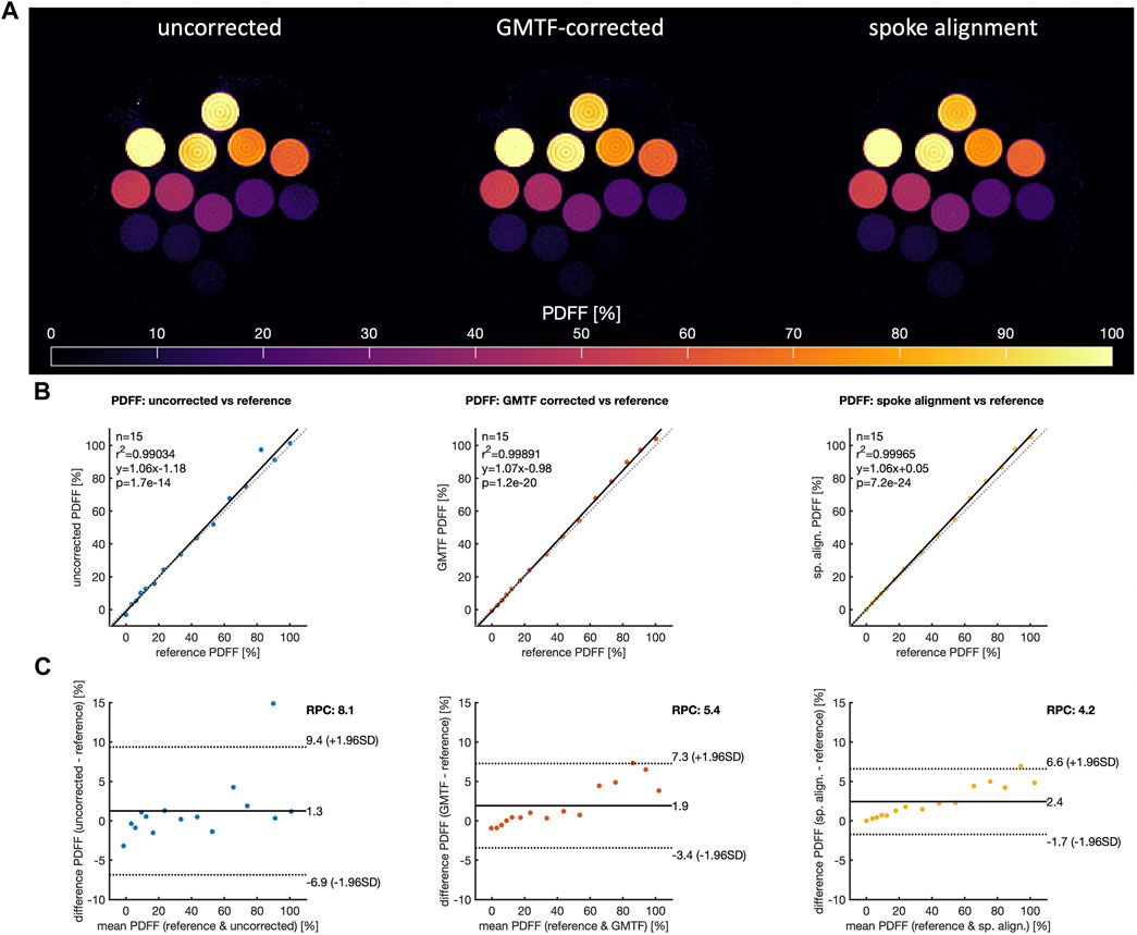
FIGURE 5. GMTF correction results of the PDFF phantom acquisition. (A) uncorrected, GMTF-corrected and spoke alignment-corrected PDFF maps. (B) linear regression comparison of PDFF values obtained from uncorrected data (left), GMTF-corrected data (center) and data corrected with the spoke alignment method (right) to the reference values. (C) corresponding Bland-Altman comparison of PDFF values to the reference values. The dashed line represents the identity in the linear regression plot, the solid black line the linear fit to the data. Bland-Altman plots: the solid black line marks the mean difference (MD), the dashed lines show the limits of agreement (LoA = MD
Applying the GMTF correction improved the linear correlation between the corrected PDFF values and the reference values with a coefficient of determination of r2 = 0.999. The LoA were narrowed down to 1.9%
Since PDFF vials with a PDFF above 50% showed larger errors in the uncorrected and corrected case than the vials below 50%, the same statistical analysis was performed separately for the lower PDFF range of 0%–50% containing 9 vials (see Figure 6). When displaying the corrected and uncorrected PDFF maps in a tighter intensity window (see Figure 6A), PDFF variations in the water-only bath around the fat fraction vials became visible. PDFF values of up to −10% were observed for the uncorrected case in the water bath region of the phantom at the right bottom edge and in locations between the high PDFF vials. Applying the GMTF correction improved the quality of the PDFF map. Linear regression comparisons to the PDFF reference values within the 0%–50% range are shown for the uncorrected, GMTF corrected and spoke alignment-corrected data in Figure 6B and the corresponding Bland-Altman comparison results in Figure 6C. Applying the GMTF correction improved the linear regression test from r2 = 0.99 to r2 = 1.00 in the 0%–50% PDFF range. The Bland-Altman analysis in the same range confirmed an improvement of the PDFF maps by the GMTF correction. MD of the uncorrected data was −0.26% with LoA of MD
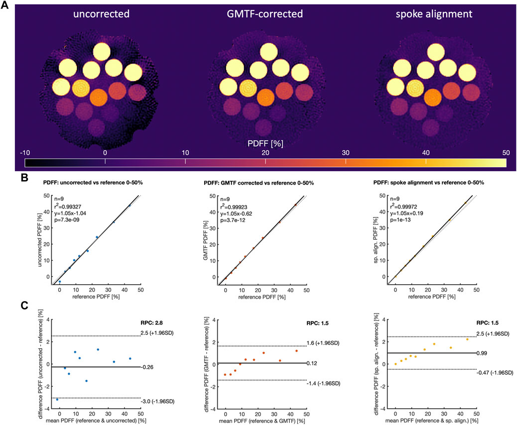
FIGURE 6. Analysis of the GMTF correction results the PDFF phantom acquisition within the 0%–50% PDFF range. (A) uncorrected, GMTF-corrected and spoke alignment-corrected PDFF maps from Figure 5 in a tighter PDFF window highlight negative PDFF quantification errors in the water area of the phantom and the 0% vial. (B) linear regression comparison of PDFF values obtained from uncorrected data (left), GMTF-corrected data (center) and data corrected with the spoke alignment method (right) to the reference values for vials with PDFF in the range 0%–50%. (C) corresponding Bland-Altman comparison of PDFF values to the reference values for vials with PDFF in the range 0%–50%. The dashed line represents the identity in the linear regression plot, the solid black line the linear fit to the data. Bland-Altman plots: the solid black line marks the mean difference (MD), the dashed lines show the limits of agreement [LoA = MD
A PDFF map comparison of the upper thigh of a healthy volunteer is displayed in Figure 7. The uncorrected PDFF map showed severe spatial inhomogeneity induced by trajectory errors at the left and right edges of the FOV causing negative PDFF values inside the muscle and quantification errors at the right edge of the right thigh. The PDFF map obtained from the data reconstructed with the proposed GMTF correction showed clear improvement over the uncorrected PDFF map. The quantification errors on the right side of the right thigh and the negative PDFF values in the left thigh could be corrected. The overall appearance of the PDFF map inside the thigh muscle was more homogeneous and in better agreement with the conventional low-resolution Cartesian acquisition. The data-driven spoke alignment approach was also able to correct for trajectory errors of the uncorrected data and achieved a comparable PDFF map quality as the GMTF correction.
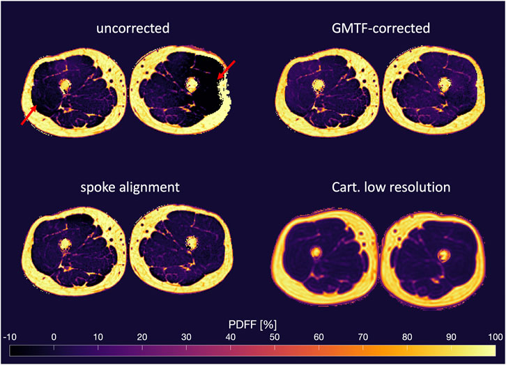
FIGURE 7. PDFF map comparison of the upper thigh of a healthy volunteer. PDFF maps obtained from uncorrected images (top left), GMRF-corrected images (top right) and images corrected with the spoke alignment method (bottom left). Bottom right: PDFF map from a low-resolution Cartesian acquisition for comparison. Negative PDFF estimation errors and inhomogeneous PDFF distributions in the muscle tissue of the uncorrected data (indicated by red arrows) are corrected with both the GMTF and the spoke alignment method.
A similar PDFF map comparison for an axial liver acquisition of a healthy volunteer is shown in Figure 8. The PDFF map derived from the uncorrected echo images of the radial SoS sequence was heavily affected by trajectory errors, resulting in PDFF inhomogeneities. Quantification errors in subcutaneous adipose tissue were particularly noticeable near the FOV’s right edge. Severe negative PDFF underestimations of up to −20% were observed at the lateral back muscles, the spleen and the right liver lobe. The overall quality of the PDFF map estimated from GMTF-corrected images was significantly higher. Errors in the right side’s subcutaneous adipose tissue were removed, and the full body outline was restored. The PDFF distribution within the liver was more homogeneous than in the uncorrected case and negative PDFF values in the spleen, right liver lobe and lateral back muscles were corrected as well. The PDFF map agreed in terms of homogeneity with the low-resolution Cartesian breath-hold acquisition. The spoke alignment correction was also able to correct most of the trajectory errors and yielded a PDFF map quality comparable to that of the GMTF correction. In the PDFF maps corrected with both the spoke alignment and the GMTF-correction methods, only minor negative PDFF underestimations were observed at fat–organ tissue and fat–muscle interfaces, as well as in motion-affected areas such as the right liver lobe and the sternum, which are challenging areas for water–fat separation. The liver ROI analysis of the corrected and uncorrected PDFF maps (Figure 9) confirmed that the GMTF correction reduced the standard deviation of the liver PDFF in comparison with the uncorrected data for each subject. After the GMTF correction, the mean liver PDFF agreed with the Cartesian reference mean PDFF within their standard deviation. Comparable correction results were observed for the spoke alignment method. The smallest correction improvements were observed in subjects 3 and 9, which also had the smallest abdominal cavity size.
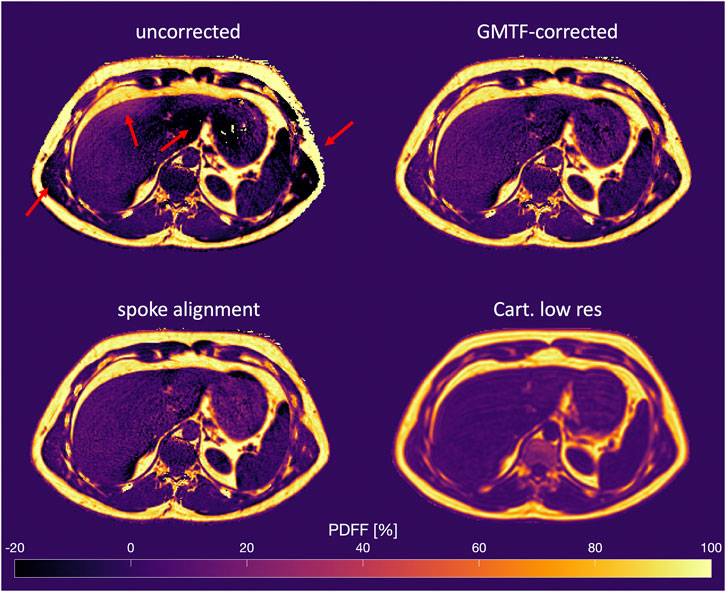
FIGURE 8. PDFF map comparison from a liver scan of a healthy volunteer. PDFF maps obtained from uncorrected images (top left), GMTF-corrected images (top right) and images corrected with the spoke alignment method (bottom left). Bottom right: PDFF map from a low-resolution Cartesian breath-hold acquisition for comparison. The red arrows highlight PDFF quantification errors for the uncorrected data. GMTF and spoke alignment method remove PDFF errors and achieve a homogeneous PDFF distribution in the liver.
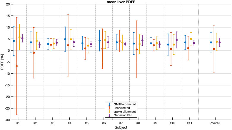
FIGURE 9. Mean liver PDFF over the different liver regions in eleven healthy volunteers. PDFF results obtained from uncorrected data (red), GMTF-corrected data (blue), data corrected with the spoke alignment method (yellow) and data from a low resolution Cartesian breath-hold acquisition (purple). The error bars represent the standard deviation over the different liver regions for a single subject. On the right the mean values over all eleven subjects are shown with the combined standard deviations.
Eddy currents and gradient system delays are known to cause PDFF quantification errors in both Cartesian [26–28] and radial [16, 17, 19, 20] acquisitions. Radial acquisitions have recently emerged as a viable approach for accomplishing free-breathing PDFF mapping. However, in radial acquisitions a correction of k-space trajectory errors induced by gradient chain imperfections is required to obtain meaningful PDFF maps. The present work shows that a GMTF-based trajectory correction can achieve robust PDFF mapping results when using a radial SoS sequence.
Most previous methods to correct for gradient chain imperfections in radial water–fat imaging relied on the acquisition of calibration lines with opposite polarity [15–21] and recently on estimating the k-space shifts from the radial raw data directly [41]. A GMTF-based trajectory correction method has been applied in cardiac PDFF mapping using a 3D radial sequence lately [61].
The proposed GMTF method provides a flexible correction method for gradient system imperfections which is independent of the applied imaging parameters. A single calibration measurement and a chirp based LTI model [32, 43, 52] are sufficient to obtain the required GMTF to characterize the gradient system chain. As shown previously a GMTF can remain stable over several years [47]. The proposed trajectory correction method could thus be applied in all subsequent image reconstructions from the same scanner without the need of additional calibration scans.
The anisotropic eddy current behavior for the respective gradient axes was measured and corrected based on the extracted GMTF. Only first-order gradient terms responsible for linear eddy currents were considered for the correction step. To include higher-order terms, the phantom method could be extended to 3D by applying phase encoding [45], or a field camera [42, 47] could be used.
The simulation results showed that trajectory errors, predicted by the GMTF measurement, cause magnitude errors in the reconstructed echo images (see Supplementary Figure S1), which translate to PDFF quantification errors. Especially the negative PDFF bias in the numerical phantom could also be observed in the corresponding uncorrected water bottle phantom scan as well as in the water area of the PDFF phantom scan. In both cases the GMTF correction was able to correct the negative PDFF bias in the water area and retrieve a homogeneous PDFF map. In general, the proposed GMTF method improved the PDFF estimation of the PDFF phantom scan, by increasing the linear correlation between the measured and reference PDFF values, as well as reducing the standard deviation of the mean difference between the measured and the reference PDFF over the full range of 0%–100% PDFF. Especially the low fat fraction range of the PDFF phantom scan illustrated the impact of the GMTF-based trajectory correction.
Both scanned in vivo anatomies, the upper thigh and the liver, showed the impact of the gradient chain induced trajectory errors on the PDFF maps and proved the need of eddy current correction for precise PDFF mapping in radial Dixon imaging. Uncorrected PDFF maps for both anatomies had significant errors in PDFF values. In both cases the proposed GMTF method was able to correct these errors and to retrieve meaningful PDFF maps. Correcting the liver acquisition data improved the PDFF estimation of the liver, by reducing the standard deviation of the mean liver PDFF across liver regions of each subject and by reducing the bias of the mean liver PDFF.
The GMTF correction achieved comparable results as the data-driven approach based on aligning radial spokes of opposite polarity. Despite comparable results, the two methods operate in different ways. The spoke alignment method can inherently correct only constant shifts along the k-space spoke. While the GMTF method is also able to correct linear phase errors by measuring trajectory shifts in k-space, these shifts are not required to be constant over the whole spoke. On the contrary, the results of the trajectory correction yielded larger shifts at the beginning and the end of each spoke, thus affecting the high spatial frequency components of the reconstructed images. While the presented data-driven approaches and methods relying on the acquisition of calibration scans can only shift k-space data, the GMTF-based correction is able to shift and warp k-space sampling positions.
Furthermore, the proposed GMTF method is faster and less computationally demanding than the spoke alignment method. While the fitting operation of the k-space shift during the spoke alignment has to be performed per imaging slice, per angle and per echo, the GMTF correction requires only a single convolution of the input gradient waveform and its integration to calculate a trajectory for a full TR. The proposed GMTF method added only a few seconds to the reconstruction pipeline. It can be thus easily added to any existing non-Cartesian reconstruction pipeline which is able to use the predicted trajectory in a gridding- or NUFFT-based reconstruction.
The present work has several limitations: First, precise knowledge of the input gradient waveform is necessary for a GMTF-based correction method to predict the real gradient waveform. Depending on the manufacturer and the applied sequence, this knowledge may require access to the pulse sequence programming. Second, the GMTF used in this work was only measured up to 10 kHz. While this range is sufficient to cover the frequencies of typical Dixon readout gradient waveforms, this may not be the case for arbitrary waveforms. In this case, a GMTF with a higher frequency range would be necessary. Third, the effect of B0 eddy currents was neglected in this work, since the main contributions were expected to stem from linear eddy currents. This correction however could be easily implemented because the B0 transfer function can be extracted from the acquired GMTF data. Fourth, geometric distortions caused by spatial nonlinearities in the gradient fields at the FOV edge are not adapted by the proposed method. These nonlinearities are static and do not account for eddy current-induced dynamic trajectory errors. Fifth, a comparison to a GMTF obtained with NMR field probes could not be investigated unfortunately due to the lack of such a field camera device [32, 34]. Sixth, all SoS acquisitions in this work were performed in the same orientation with the SoS axis being aligned with the z-direction. When using double-oblique orientations, the trajectory can be corrected with the GMTF, but 3D encoding and 3D gridding have to be used instead of 2D gridding. Finally, GMTF correction was only evaluated on a pool of healthy volunteers with normal PDFF values. A further clinical evaluation of patients with increased liver PDFF would be of interest.
The present work showed that a simple phantom-based GMTF measurement without any additional scanner hardware can be used to correct k-space trajectories in radial SoS Dixon acquisitions for gradient system imperfections. It was demonstrated that the GMTF-based trajectory correction improves PDFF quantification in radial SoS Dixon acquisitions in phantoms and in vivo.
The datasets presented in this article are not readily available because the in vivo data cannot be shared according to the ethics approval. The phantom data can be shared upon request. Basic GMTF measurement results from a Philips system and means to efficiently obtain them are published in (JR, Mazurkewitz P, PB, Nielsen T. Magn Reson Med. 2019 Dec; 82(6):2146-2159). Requests to access the datasets should be directed to christoph.zoellner@tum.de, www.bmrr.de.
The studies involving humans were approved by the ethics committee of Klinikum rechts der Isar, Technical University of Munich, Munich, Germany. The studies were conducted in accordance with the local legislation and institutional requirements. The participants provided their written informed consent to participate in this study.
CZ, SK, and DK conceived and planned the project. JR and PB developed and provided the fundamentals of the GMTF measurement method. CZ carried out all measurements, performed the numerical simulations, processed and analyzed the data. CB and JS designed the water-fat separation code. KW, JP, SK, DJ, and DK aided in interpreting the results. CZ drafted the manuscript and designed the figures with input from all authors. All authors contributed to the article and approved the submitted version.
The present work received funding support by the German Research Foundation (project number 455422993, FOR5298-iMAGOP1 and SFB824/A9).
The authors would like to acknowledge Dr. Stefan Ruschke and Dr. Shuo Zhang for helpful discussions. The authors would like to thank Dr. Peter Mazurkewitz for help with the GMTF measurement technique. The authors would finally like to acknowledge general research support from Philips Healthcare.
The authors KW, JR, PB, and JP are employed by Philips. DK receives research funding from Philips Healthcare outside the scope of the present manuscript.
The remaining authors declare that the research was conducted in the absence of any commercial or financial relationships that could be construed as a potential conflict of interest.
All claims expressed in this article are solely those of the authors and do not necessarily represent those of their affiliated organizations, or those of the publisher, the editors and the reviewers. Any product that may be evaluated in this article, or claim that may be made by its manufacturer, is not guaranteed or endorsed by the publisher.
The Supplementary Material for this article can be found online at: https://www.frontiersin.org/articles/10.3389/fphy.2023.1124980/full#supplementary-material
1. Bley TA, Wieben O, François CJ, Brittain JH, Reeder SB. Fat and water magnetic resonance imaging. J Magn Reson Imaging (2010) 31(1):4–18. doi:10.1002/jmri.21895
2. Hu HH, Branca RT, Hernando D, Karampinos DC, Machann J, McKenzie CA, et al. Magnetic resonance imaging of obesity and metabolic disorders: Summary from the 2019 ISMRM Workshop. Magn Reson Med (2020) 83(5):1565–76. doi:10.1002/mrm.28103
3. Liu CY, McKenzie CA, Yu H, Brittain JH, Reeder SB. Fat quantification with IDEAL gradient echo imaging: correction of bias from T1 and noise. Magn Reson Med (2007) 58(2):354–64. doi:10.1002/mrm.21301
4. Karampinos DC, Yu H, Shimakawa A, Link TM, Majumdar S. T1-corrected fat quantification using chemical shift-based water/fat separation: application to skeletal muscle. Magn Reson Med (2011) 66(5):1312–26. doi:10.1002/mrm.22925
5. Yu H, McKenzie CA, Shimakawa A, Vu AT, Brau AC, Beatty PJ, et al. Multiecho reconstruction for simultaneous water-fat decomposition and T2* estimation. J Magn Reson Imaging (2007) 26(4):1153–61. doi:10.1002/jmri.21090
6. Bydder M, Yokoo T, Hamilton G, Middleton MS, Chavez AD, Schwimmer JB, et al. Relaxation effects in the quantification of fat using gradient echo imaging. Magn Reson Imaging (2008) 26(3):347–59. doi:10.1016/j.mri.2007.08.012
7. Berglund J, Kullberg J. Three-dimensional water/fat separation and T 2 * estimation based on whole-image optimization-Application in breathhold liver imaging at 1.5 T. Magn Reson Med (2012) 67(6):1684–93. doi:10.1002/mrm.23185
8. Yu H, Shimakawa A, McKenzie CA, Brodsky E, Brittain JH, Reeder SB. Multiecho water-fat separation and simultaneous R*2 estimation with multifrequency fat spectrum modeling. Magn Reson Med (2008) 60(5):1122–34. doi:10.1002/mrm.21737
9. Yu H, Shimakawa A, Hines CDG, McKenzie CA, Hamilton G, Sirlin CB, et al. Combination of complex-based and magnitude-based multiecho water-fat separation for accurate quantification of fat-fraction. Magn Reson Med (2011) 66(1):199–206. doi:10.1002/mrm.22840
10. Peterson P, Månsson S. Fat quantification using multiecho sequences with bipolar gradients: Investigation of accuracy and noise performance. Magn Reson Med (2014) 71(1):219–29. doi:10.1002/mrm.24657
11. Reeder SB, Cruite I, Hamilton G, Sirlin CB. Quantitative assessment of liver fat with magnetic resonance imaging and spectroscopy. J Magn Reson Imaging (2011) 34(4):729–49. doi:10.1002/jmri.22580
12. Hu HH, Yokoo T, Bashir MR, Sirlin CB, Hernando D, Malyarenko D, et al. Linearity and bias of proton density fat fraction as a quantitative imaging biomarker: A multicenter, multiplatform, multivendor phantom study. Radiology (2021) 298(3):640–51. doi:10.1148/radiol.2021202912
13. Syväri J, Junker D, Patzelt L, Kappo K, Al Sadat L, Erfanian S, et al. Longitudinal changes on liver proton density fat fraction differ between liver segments. Quant Imaging Med Surg (2021) 11(5):1701–9. doi:10.21037/qims-20-873
14. Block KT, Chandarana H, Milla S, Bruno M, Mulholland T, Fatterpekar G, et al. Towards routine clinical use of radial stack-of-stars 3D gradient-echo sequences for reducing motion sensitivity. J Korean Soc Magn Reson Med (2014) 18(2):87. doi:10.13104/jksmrm.2014.18.2.87
15. Benkert T, Feng L, Sodickson DK, Chandarana H, Block KT. Free-breathing volumetric fat/water separation by combining radial sampling, compressed sensing, and parallel imaging. Magn Reson Med (2017) 78(2):565–76. doi:10.1002/mrm.26392
16. Armstrong T, Dregely I, Stemmer A, Han F, Natsuaki Y, Sung K, et al. Free-breathing liver fat quantification using a multiecho 3D stack-of-radial technique. Magn Reson Med (2018) 79(1):370–82. doi:10.1002/mrm.26693
17. Armstrong T, Ly KV, Ghahremani S, Calkins KL, Wu HH. Free-breathing 3-D quantification of infant body composition and hepatic fat using a stack-of-radial magnetic resonance imaging technique. Pediatr Radiol (2019) 49(7):876–88. doi:10.1007/s00247-019-04384-7
18. Zhong X, Armstrong T, Nickel MD, Kannengiesser SA, Pan L, Dale BM, et al. Effect of respiratory motion on free-breathing 3D stack-of-radial liver relaxometry and improved quantification accuracy using self-gating. Magn Reson Med (2020) 83(6):1964–78. doi:10.1002/mrm.28052
19. Zhong X, Hu HH, Armstrong T, Li X, Lee YH, Tsao TC, et al. Free-breathing volumetric liver R2* and ProtonDensity fat fraction quantification in pediatric patients using stack-of-radial MRI with self-gating motion compensation. J Magn Reson Imaging (2020) 53:118–29. doi:10.1002/jmri.27205
20. Armstrong T, Ly KV, Murthy S, Ghahremani S, Kim GHJ, Calkins KL, et al. Free-breathing quantification of hepatic fat in healthy children and children with nonalcoholic fatty liver disease using a multi-echo 3-D stack-of-radial MRI technique. Pediatr Radiol (2018) 48(7):941–53. doi:10.1007/s00247-018-4127-7
21. Schneider M, Benkert T, Solomon E, Nickel D, Fenchel M, Kiefer B, et al. Free-breathing fat and R2* quantification in the liver using a stack-of-stars multi-echo acquisition with respiratory-resolved model-based reconstruction. Magn Reson Med (2020) 84(5):2592–605. doi:10.1002/mrm.28280
22. Peters DC, Derbyshire JA, McVeigh ER. Centering the projection reconstruction trajectory: Reducing gradient delay errors. Magn Reson Med (2003) 50(1):1–6. doi:10.1002/mrm.10501
23. Moussavi A, Untenberger M, Uecker M, Frahm J. Correction of gradient-induced phase errors in radial MRI. Magn Reson Med (2014) 71(1):308–12. doi:10.1002/mrm.24643
24. Block KT, Uecker M. Simple method for adaptive gradient-delay compensation in radial MRI. Proc Intl Soc Magn Reson Med (2011) 19:2816.
25. Hernando D, Liang ZP, Kellman P. Chemical shift-based water/fat separation: A comparison of signal models. Magn Reson Med (2010) 64(3):811–22. doi:10.1002/mrm.22455
26. Yu H, Shimakawa A, McKenzie CA, Lu W, Reeder SB, Hinks RS, et al. Phase and amplitude correction for multi-echo water-fat separation with bipolar acquisitions. J Magn Reson Imaging (2010) 31(5):1264–71. doi:10.1002/jmri.22111
27. Hernando D, Hines CDG, Yu H, Reeder SB. Addressing phase errors in fat-water imaging using a mixed magnitude/complex fitting method. Magn Reson Med (2012) 67(3):638–44. doi:10.1002/mrm.23044
28. Ruschke S, Eggers H, Kooijman H, Diefenbach MN, Baum T, Haase A, et al. Correction of phase errors in quantitative water–fat imaging using a monopolar time-interleaved multi-echo gradient echo sequence. Magn Reson Med (2017) 78(3):984–96. doi:10.1002/mrm.26485
29. De Zanche N, Barmet C, Nordmeyer-Massner JA, Pruessmann KP. NMR Probes for measuring magnetic fields and field dynamics in MR systems. Magn Reson Med (2008) 60(1):176–86. doi:10.1002/mrm.21624
30. Dietrich BE, Brunner DO, Wilm BJ, Barmet C, Gross S, Kasper L, et al. A field camera for MR sequence monitoring and system analysis. Magn Reson Med (2016) 75(4):1831–40. doi:10.1002/mrm.25770
31. Vannesjo SJ, Dietrich BE, Pavan M, Brunner DO, Wilm BJ, Barmet C, et al. Field camera measurements of gradient and shim impulse responses using frequency sweeps. Magn Reson Med (2014) 72(2):570–83. doi:10.1002/mrm.24934
32. Addy NO, Wu HH, Nishimura DG. Simple method for MR gradient system characterization and k-space trajectory estimation. Magn Reson Med (2012) 68(1):120–9. doi:10.1002/mrm.23217
33. Duyn JH, Yang Y, Frank JA, Van Der Veen JW. Simple correction method for k-space trajectory deviations in MRI. J Magn Reson (1998) 132(1):150–3. doi:10.1006/jmre.1998.1396
34. Beaumont M, Lamalle L, Segebarth C, Barbier EL. Improved k-space trajectory measurement with signal shifting. Magn Reson Med (2007) 58(1):200–5. doi:10.1002/mrm.21254
35. Robison RK, Devaraj A, Pipe JG. Fast, simple gradient delay estimation for spiral MRI. Magn Reson Med (2010) 63(6):1683–90. doi:10.1002/mrm.22327
36. Deshmane A, Blaimer M, Breuer F, Jakob P, Duerk J, Seiberlich N, et al. Self-calibrated trajectory estimation and signal correction method for robust radial imaging using GRAPPA operator gridding. Magn Reson Med (2016) 75(2):883–96. doi:10.1002/mrm.25648
37. Krämer M, Biermann J, Reichenbach JR. Intrinsic correction of system delays for radial magnetic resonance imaging. Magn Reson Imaging (2015) 33(4):491–6. doi:10.1016/j.mri.2015.01.005
38. Lee KJ, Paley MNJ, Griffiths PD, Wild JM. Method of generalized projections algorithm for image-based reduction of artifacts in radial imaging. Magn Reson Med (2005) 54(1):246–50. doi:10.1002/mrm.20554
39. Rosenzweig S, Holme HCM, Uecker M. Simple auto-calibrated gradient delay estimation from few spokes using Radial Intersections (RING). Magn Reson Med (2019) 81(3):1898–906. doi:10.1002/mrm.27506
40. Untenberger M, Tan Z, Voit D, Joseph AA, Roeloffs V, Merboldt KD, et al. Advances in real-time phase-contrast flow MRI using asymmetric radial gradient echoes. Magn Reson Med (2016) 75(5):1901–8. doi:10.1002/mrm.25696
41. Tan Z, Unterberg-Buchwald C, Blumenthal M, Scholand N, Schaten P, Holme C, et al. Free-breathing water, fat, R2* and B0 field mapping of the liver using multi-echo radial FLASH and regularized model-based reconstruction (MERLOT) (2021). p. 1–29.
42. Vannesjo SJ, Haeberlin M, Kasper L, Pavan M, Wilm BJ, Barmet C, et al. Gradient system characterization by impulse response measurements with a dynamic field camera. Magn Reson Med (2013) 69(2):583–93. doi:10.1002/mrm.24263
43. Liu H, Matson GB. Accurate measurement of magnetic resonance imaging gradient characteristics. Materials (Basel) (2014) 7:1–15. doi:10.3390/ma7010001
44. Brodsky EK, Klaers JL, Samsonov AA, Kijowski R, Block WF. Rapid measurement and correction of phase errors from B0 eddy currents: Impact on image quality for non-cartesian imaging. Magn Reson Med (2013) 69(2):509–15. doi:10.1002/mrm.24264
45. Rahmer J, Mazurkewitz P, Börnert P, Nielsen T. Rapid acquisition of the 3D MRI gradient impulse response function using a simple phantom measurement. Magn Reson Med (2019) 82(6):2146–59. doi:10.1002/mrm.27902
46. Gurney P, Pauly J, Nishimura DG. A simple method for measuring B0 eddy currents. Proc 13th Annu Meet ISMRM (2005) 13:866.
47. Vannesjo SJ, Graedel NN, Kasper L, Gross S, Busch J, Haeberlin M, et al. Image reconstruction using a gradient impulse response model for trajectory prediction. Magn Reson Med (2016) 76(1):45–58. doi:10.1002/mrm.25841
48. Prince JL, Links JM. Upper Saddle River: Pearson Prentice Hall (2006).Medical imaging signals and systems
49. Brodsky EK, Samsonov AA, Block WF. Characterizing and correcting gradient errors in non-Cartesian imaging: Are gradient errors Linear Time-Invariant (LTI)? Magn Reson Med (2009) 62(6):1466–76. doi:10.1002/mrm.22100
50. Kronthaler S, Rahmer J, Börnert P, Makowski MR, Schwaiger BJ, Gersing AS, et al. Trajectory correction based on the gradient impulse response function improves high-resolution UTE imaging of the musculoskeletal system. Magn Reson Med (2021) 85(4):2001–15. doi:10.1002/mrm.28566
51. Wilm BJ, Barmet C, Pavan M, Pruessmann KP. Higher order reconstruction for MRI in the presence of spatiotemporal field perturbations. Magn Reson Med (2011) 65(6):1690–701. doi:10.1002/mrm.22767
52. Campbell-Washburn AE, Xue H, Lederman RJ, Faranesh AZ, Hansen MS. Real-time distortion correction of spiral and echo planar images using the gradient system impulse response function. Magn Reson Med (2016) 75(6):2278–85. doi:10.1002/mrm.25788
53. Hedderich DM, Weiss K, Spiro J, Giese D, Beck G, Maintz D, et al. Clinical evaluation of free-breathing contrast-enhanced T1w MRI of the liver using pseudo golden angle radial k-space sampling. Rofo Fortschritte auf Dem Gebiet der Rontgenstrahlen der Bildgeb Verfahren (2018) 190(7):601–9. doi:10.1055/s-0044-101263
54. Pruessmann KP, Weiger M, Scheidegger MB, Boesiger P. Sense: Sensitivity encoding for fast MRI. Magn Reson Med (1999) 42(5):952–62. doi:10.1002/(sici)1522-2594(199911)42:5<952:aid-mrm16>3.0.co;2-s
55. Uecker M, Ong F, Tamir JI, Bahri D, Virtue P, Cheng JY, et al. Berkeley advanced reconstruction toolbox. Proc Intl Soc Mag Reson Med (2015) 23:2486. doi:10.5281/zenodo.592960
56. Boehm C, Diefenbach MN, Makowski MR, Karampinos DC. Improved body quantitative susceptibility mapping by using a variable-layer single-min-cut graph-cut for field-mapping. Magn Reson Med (2021) 85(3):1697–712. doi:10.1002/mrm.28515
57. Bydder M, Girard O, Hamilton G. Mapping the double bonds in triglycerides. Magn Reson Imaging (2011) 29(8):1041–6. doi:10.1016/j.mri.2011.07.004
58. Hamilton G, Yokoo T, Bydder M, Cruite I, Schroeder ME, Sirlin CB, et al. In vivocharacterization of the liver fat1H MR spectrum: IN vivocharacterization of the liver FAT1H MR spectrum. NMR Biomed (2011) 24(7):784–90. doi:10.1002/nbm.1622
59. Hamilton G, Schlein AN, Middleton MS, Hooker CA, Wolfson T, Gamst AC, et al. In vivo triglyceride composition of abdominal adipose tissue measured by 1H MRS at 3T. J Magn Reson Imaging (2017) 45(5):1455–63. doi:10.1002/jmri.25453
60. Campo CA, Hernando D, Schubert T, Bookwalter CA, Van Pay AJ, Reeder SB. Standardized approach for ROI-based measurements of proton density fat fraction and r2 in the liver. Am J Roentgenol (2017) 209(3):592–603. doi:10.2214/ajr.17.17812
Keywords: eddy currents, gradient delays, k-space trajectory distortions, radial, stack-of-stars, proton density fat fraction (PDFF), Dixon imaging, magnetic resonance imaging (MRI)
Citation: Zöllner C, Kronthaler S, Weiss K, Boehm C, Stelter J, Rahmer J, Börnert P, Peeters JM, Junker D and Karampinos DC (2023) Correcting gradient chain induced fat quantification errors in radial multi-echo Dixon imaging using a gradient modulation transfer function. Front. Phys. 11:1124980. doi: 10.3389/fphy.2023.1124980
Received: 15 December 2022; Accepted: 11 September 2023;
Published: 27 September 2023.
Edited by:
J. H. Gao, Peking University, ChinaReviewed by:
Yanjie Zhu, Chinese Academy of Sciences (CAS), ChinaCopyright © 2023 Zöllner, Kronthaler, Weiss, Boehm, Stelter, Rahmer, Börnert, Peeters, Junker and Karampinos. This is an open-access article distributed under the terms of the Creative Commons Attribution License (CC BY). The use, distribution or reproduction in other forums is permitted, provided the original author(s) and the copyright owner(s) are credited and that the original publication in this journal is cited, in accordance with accepted academic practice. No use, distribution or reproduction is permitted which does not comply with these terms.
*Correspondence: Christoph Zöllner, Y2hyaXN0b3BoLnpvZWxsbmVyQHR1bS5kZQ==
Disclaimer: All claims expressed in this article are solely those of the authors and do not necessarily represent those of their affiliated organizations, or those of the publisher, the editors and the reviewers. Any product that may be evaluated in this article or claim that may be made by its manufacturer is not guaranteed or endorsed by the publisher.
Research integrity at Frontiers
Learn more about the work of our research integrity team to safeguard the quality of each article we publish.