 Fujun Lai
 Sicheng Li
 Liang Lv1
 Sha Zhu
- 1School of Finance, Yunnan University of Finance and Economics, Kunming, China
- 2School of Statistics and Mathematics, Yunnan University of Finance and Economics, Kunming, China
Based on the Vector Autoregressive Model (VAR), this paper constructs a contagion complex network of global stock market returns, and uses the Quantile-on-Quantile Regression (QQR) to explore the impact of global geopolitical risks on the connectedness of global stock markets. By applying the risk contagion analysis framework, we depict risk contagion and correlation between financial markets in different countries. We also identify the risk contagion characteristics of international financial markets. This paper innovatively introduces the quantile-on-quantile regression method to the study of geopolitical risk. Through the quantile-on-quantile approach, we find that there is an asymmetric relationship between geopolitical risk and the global stock market correlation network. Our conclusions provide some suggestions for policy makers and relevant investors on how to deal with the current high global geopolitical risks. They also provide ideas on how to effectively hedge such risks during asset allocation and policy formulation.
1 Introduction
Since the collapse of the Soviet Union in the early 1990s, the Cold War crisis has been lifted. The world pattern of two superpowers has been replaced by a single superpower. Nevertheless, all of this does not appear to be reducing global geopolitical risk. Peace is something of a mirage in the short-term, while disputes and conflicts remain the defining features of the world. Because of the one superpower and many powers pattern, the relationship between the major powers has become tense, and conflicts between small countries have also risen. The outbreak of the Russia-Ukraine conflict in early 2022 has further disrupted a world that is already affected by COVID-19. As the world’s dramatic changes continue to accelerate, geopolitical risks will continue to grow.
Numerous scholars have provided different definitions of geopolitical risk, but until today, there is no unified understanding or definition. The earliest geopolitics originated in the late 19 th century, and was proposed by Swedish political geographer Johan Rudolf Kjellén in his book Der Staat als Lebensform (1917). Since the 20th century, due to the development of global politics, economy and military, various geopolitical theories have emerged. American historian Mahan put forward the sea power theory, who can control the sea, who can become a world power; the key to controlling the ocean is to control the world‘s critical sea lanes and straits. Mackinder put forward the land rights theory, that with the development of land transportation, the heartland of Eurasia has become the most critical strategic area. The land power theory has had a profound impact on world politics. In the 1940s, American international relations scholar Spykman emphasized the importance of rimland and carried forward continental margin theory, which was called another theory of continental power theory. In the 1950 s, American strategist Seversky put forward the theory that the Arctic region is very important for the United States to compete for air supremacy, namely air power theory. In 1973, American geographer Cohen proposed the geopolitical strategic zone model, which divided the world into two geopolitical strategic zones: maritime trade zone and Eurasian continental zone. Between the two regions there are three regions: South Asia, the Middle East and Southeast Asia. South Asia is a potential geostrategic region, and the Middle East and Southeast Asia are called fracture zones. In 1982, Cohen proposed a revision of the geopolitical strategic zone model, noting that Western European countries, Japan, and China had developed into world powers; the role and status of India, Brazil, and Nigeria had risen; and sub-Saharan South Africa had transformed into a third fracture zone.
The World Economic Forum in Davos releases the Global Risk Report every year. In the 2015 edition of the Global Risk Report, geopolitical risk is defined as a systematic, cross-regional and cross-industry global risk, covering violent conflicts between countries, civil strife in important countries, large-scale terrorist attacks, proliferation of weapons of mass destruction and failure of global governance. The 2019 edition of the Global Risks Report lists some specific manifestations of geopolitical risks, such as national collapse or crisis, national governance failure, regional or global governance failure, inter-state conflicts, and terrorist attacks.
David K. Bohl [1] defines geopolitical risks as trends in political and economic changes that are potentially destructive to human well being, arguing that geopolitical risks stem from three interrelated risks: first, political risks arising from competition for power among geopolitical actors, the most intense manifestation of which is violent conflict, but may also include other forms of destructive competition; second, economic risks caused by global or regional economic and financial turmoil; third, natural risks caused by non-human environmental changes, such as water shortage caused by climate change. Geopolitical risks arise not only within a single risk, but also from the contagion between risks. For example, water shortage (a natural risk) may lead to military tension (a political risk), resulting in trade disruption (an economic risk).
If we only focus on the geopolitical context of the text, maybe we will not be able to better incorporate it into the economic sphere. Fortunately, Caldara and Iacoviello [2] used big data and text-mining techniques to create a quantitative standard for geopolitical events and associated risks based directly on textual analysis of news papers. They define global geopolitical risk as the threat, realization and escalation risk caused by adverse events related to war, terrorism, and tensions between countries. These events affect the peace process in international relations. Furthermore, they classify global geopolitical risks into global geopolitical threat risk and global geopolitical act risks. Global geopolitical threats include war threats, peace threats, military build-ups, nuclear threats and terrorist threats. Global geopolitical acts include the beginning of war, the escalation of war and terrorist acts. Based on this, three indexes, global geopolitical threat risk, global geopolitical act risk and global geopolitical risk are constructed. In order to quantify the magnitude of global geopolitical risks, Caldara and Iacoviello [2] retrieved 25 million articles published in major international English newspapers since 1900. And they calculated the frequency of occurrence of words related to geopolitical events and related threats every month, and then standardized them, and finally obtained the monthly global geopolitical risk (GPR) index. In summary, the definition of geopolitical risk has not been unified. However, this article draws on the global geopolitical risk index measured by Caldara and Iacoviello [2], so we use their definition of geopolitical risk.
Since the establishment of the geopolitical risk index, a large number of scholars have conducted various empirical studies [3–11]. World financial market volatility and even macroeconomic cycles are strongly influenced by geopolitical risk. Geopolitical risk shocks are always accompanied by periods of high risk on financial markets. There are two direct and indirect channels for this transmission. In the direct channel, after geopolitical risk increases, it will affect the financial market and reduce credit demand through cross-border capital flows, exchange rate fluctuations, large fluctuations in commodity prices (crude oil), and asset price adjustments (stocks and real estate). In terms of indirect channels, most people are averse to the uncertainty created by rising geopolitical risk, which will undoubtedly dampen consumer and investor enthusiasm. High geopolitical uncertainty may lead to lower employment and output. Consumers may delay consumption, and businesses may delay investment because of precautionary savings motives. As a result of the geopolitical risk shock, the decline in economic activity will inevitably be reflected in the financial markets. Especially when extreme events occur, there is a huge impact on the global capital market and economic environment. For example, during the three oil crises in 1973, 1979 and 1990, three major geopolitical conflicts broke out at the same time, namely, the fourth Middle East war between Arab countries and Israel, the Iran-Iraq war between Iran and Iraq, and Iraq’s invasion of Kuwait war. The three major conflicts have greatly damaged global economic growth, with global GDP growth rates falling from 6.4%, 4.2%, and 4.6%–0.6%, 0.4%, and 1.5%, respectively.
Current research on global geopolitical risks mainly focuses on energy prices and stock market returns. However, the impact on the entire international stock market as a whole has not been involved. The global economy plays different roles across various industrial chains in the context of globalization. At the same time, because of the need for investment diversification, a large amount of money is invested in different stock markets to hedge risks. As a result, it is difficult for any stock market to be immune to world geopolitical shocks. Global stock markets are closely related. Stock market correlations have always played an influential role in the study of systemic financial risk. The 2008 subprime mortgage crisis accelerated the contagion of U. S. stock price volatility to the world capital markets, resulting in global stock market turbulence. In recent years, with the continuous development of modern econometric methods, examining the risk contagion effect from the perspective of complex networks has become an emerging research topic in this field. Diebold and Yilmaz [12,13] developed a risk spillover network analysis method, which can more deeply reflect the price volatility spillover effect of financial markets. With the help of this risk contagion analysis framework, we can not only depict the intensity and correlation of risk contagion between different financial sectors, but also identify the core path of risk contagion.
Geopolitical risk is undoubtedly a systemic shock that has an impact on worldwide equity markets. The impact of this natural external impact on international stock market complex networks is an issue that researchers in the academic community should focus on. For example, after the Russia-Ukraine conflict, global stock markets experienced significant volatility. However, unfortunately, no scholars have conducted in-depth research and analysis on this issue. Therefore, this paper focuses on the relationship between global geopolitical risk and the connectedness (correlation) of the entire international stock market return network. According to the best of our knowledge, this is the first paper to focus on the impact of global geopolitical risk on the connectedness (correlation) of the entire international stock market. By using the quantile-on-quantile approach, this paper aims to illustrate the asymmetric relationship between different geopolitical risk shocks and different global stock market correlations.
The main contributions of this paper are as follows. First, in contrast to Li [8], although they also use complex networks to explore the relationship between stock market, crude oil market and geopolitical risks, they focused more on the Chinese stock market and use the nonlinear Granger causality test to analyze the potential nonlinear relationship between the three variables. They also identified the main risk sources and risk transfer paths and the lead-lag relationship between geopolitical risks, crude oil and the Chinese stock market. We focus more on how global geopolitical risks affect the total spillover effect (correlation) of the overall international stock market and quantitatively analyze the relationship between them. Second, we innovatively introduce the quantile-on-quantile regression approch into the study of geopolitical risk. The construction of the geopolitical risk index provides a better quantitative indicator of geopolitical risk. This enables us to investigate how different levels of geopolitical risk will affect the connectedness of the overall international stock market. Through the quantile-on-quantile method, it can further characterize the asymmetric potential links between geopolitical risks at different levels and global stock market networks with different degrees of tightness, so as to deeply explore the causal relationship in various states. Third, we not only study the impact of the global geopolitical risk index on the correlation of global stock prices, but also study their differential impact on the correlation of global stock markets by deconstructing GPR into the global geopolitical action risk index and the global geopolitical threat risk index. We find that global geopolitical threat risk and global geopolitical action risk have significantly varying effects on the correlation of global stock markets.
The rest of this article is organized as follows. Section 2 gives a brief literature review. Section 3 introduces the data source and description, and Section 4 summarizes the model and method. Sections 5, 6 provide empirical results and conclusions.
2 Literature review
In recent years, more and more scholars begin to pay attention to the impact of geopolitical risk on financial markets. On the one hand, it is because Caldara and Iacoviello [2] constructed a quantitative geopolitical risk index, which provides a solution for more specific quantitative exploration of the impact of geopolitical risks on financial markets. On the other hand, this is also because global geopolitical risks are at an elevated level, and their impact on financial markets is becoming more extensive and profound. As the core energy resource of human society, oil is financialized at the same time, making it an influential underlying asset in the financial market. Moreover, oil itself is also associated with geopolitics, since a substantial number of geopolitical conflicts often involve competition for crude oil. Therefore, a variety of academic papers attempt to clarify the relationship between oil prices and geopolitical risks [5,6,14,15]. The results indicate that the relationship may be positive or negative. Abdel-Latif and El-Gamal [16] argue that falling oil prices also raise geopolitical risks. For net oil importers, the rise in oil prices will increase their own geopolitical risks, because they cannot bear the cost of soaring oil prices [11]. The impact of oil on geopolitical risks is not always one-way. Many people have explored how geopolitical risks affect oil prices or their volatility. A large number of scholars have adopted mathematical models to predict oil returns and volatility using geopolitical risks [18–20].
Other scholars have given ways in which geopolitical risks can affect stock markets [8,21–25], that is, using nonlinear Granger causality tests and complex network models, they demonstrated that geopolitical risks can affect stock prices by affecting oil prices. The approach at least provides a way of thinking about the causal relationship between geopolitical risks and global stock markets, regardless of whether it accurately describes reality.
Meanwhile, academic communities have been exploring the impact of terrorist activities on stock markets since the 9/11 incident [26–30]. According to most studies, terrorist activity negatively impacts stock returns, and these effects are primarily evident in traditional financial markets and developing countries. There is, however, a limitation to these studies in that they only focus on terrorism. Other geopolitical risks, such as policy risks and war risks, also contribute significantly to the volatility of financial markets. Moreover, these studies only focus on developed countries and ignore emerging market economies. In fact, emerging markets are more vulnerable to geographical shocks.
For example, Balcilar et al. [3] studied the impact of geopolitical risks on stock returns and volatility in the BRICS countries (Brazil, Russia, India, China and South Africa) through the nonparametric causality quantile method. They found that geopolitical risk has a nonlinear and asymmetric effect on market returns in different emerging economies, but a consistent effect on volatility. Hoque and Zaidi [31] employed the Markov Switching Model to find that the global geopolitical risk index and the country-specific geopolitical risk index have completely different effects on the stock markets of emerging economies. The global geopolitical risk index has both positive and negative effects on the stock markets of these emerging economies, but the country-specific geopolitical risk index has a negative impact without exception. Some scholars have also tried to use the geopolitical risk index to predict some indicators of financial markets. Apergis [32] first used a k-order nonparametric causality test to analyze whether geopolitical risks can predict stock returns and volatility of global defense companies. The results show that there is no evidence that the predictability of stock returns of these defense companies comes from geopolitical risks, but it can affect the risk profile of the company for some time to come. By adjusting the frequency of using the geopolitical risk index, especially the mixed frequency, the robustness and reliability of this prediction can be effectively improved [33]. Salisu [34] used the GRACH-MIDAS method to predict stock return volatility in 23 emerging economies with geopolitical risks. The results show that the stock markets of these emerging economies have experienced sharp fluctuations under the influence of high geopolitical risks. Zhang and Hamori [35] directly explored the spillover effects of the geopolitical risk index of the BRICS countries on some macroeconomic variables in the United States by using the extended network analysis method. The results show that the geopolitical risks of China and Russia are the main sources affecting the US stock market and volatility. Sohag [10] focused his research on green energy stocks and green bonds. The results show that geopolitical risk has a positive spillover effect on green energy stocks and green bonds. He believes that this is because investors tend to invest in these environmentally friendly assets during the period of geopolitical risk, so as to achieve risk hedging. We can see that the use of geopolitical indexes to directly study the stock market is very limited, and the focus is primarily on stock return and volatility. However, before this, Baker et al. [36] constructed economic policy uncertainty similar to the geopolitical risk index based on news texts, and many scholars have also used economic policy uncertainty to carry out corresponding research, proving that economic policy uncertainty has a strong negative impact on stock returns (Arouri et al., 2016; Brogaard and Detzel, 2015; Kang et al., 2017). Some economic policies themselves, however, have some endogenous interference with the stock market. We hope to examine the impact of external shocks on it more. Das [37]’s research using the quantile regression method shows that whether it is geopolitical risk or economic policy uncertainty, the impact of the two shocks on the stock market at different quantiles is indeed heterogeneous, and this effect is more manifested in the mean of the return rather than the variance. Based on the above research content, this paper will focus on how global geopolitical risk index impact on the return connectedness between international stock markets under different quantiles of them.
3 Data and description
The stock market index is based on 12 major global stock market indices, including: IBOVESPA (Brazil), DJI (United States), IXIC (United States), SPX (United States), FTSE (United Kingdom), FCHI (France), GDAXI (Germany), N225 (Japan), KS11 (Korea), HIS (Hong Kong, China), SENSE (India), SSEC (China). The data sample interval is from January 1991 to June 2022, which is derived from the Wind database.
This paper uses the global geopolitical risk index created by Caldara and Iacoviello [2] to measure the degree of geopolitical risk. Based on Saiz and Simonsohn [38] and Baker et al. [36], the index uses the share of articles on geopolitical events affecting the peaceful development of international relations such as terrorist attacks and wars reported by 10 newspapers published in the United States, Britain and Canada to construct the daily and monthly geopolitical risks of the world and some countries since 1900. Caldara and Iacoviello [2] also constructed two sub-components of global geopolitical threat risk (GPPT) and global geopolitical action risk (GPRA) to distinguish different global geopolitical risks. Articles in the GPRT index search include phrases related to threats and military buildups, while the GPRA index search involves phrases that implement or upgrade adverse events. The index is now widely used in academia [39–41]. The data interval is from March 1995 to June 2022.
Table 1 provides descriptive statistics for the data.
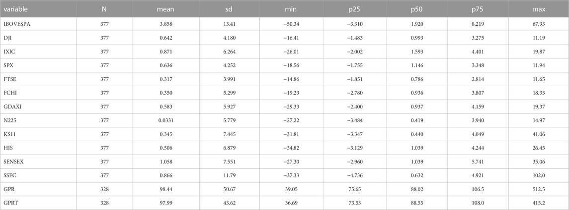
TABLE 1. Statistical description.
4 Methodology
4.1 Complex dynamic contagion network of global stock market returns
Using the Vector Autoregressive Model (VAR) method, Diebold and Yilmaz [12,13] constructed an information spillover network between financial institutions, and then implemented the rolling window method to build a continuous-time correlation network. We use this method to construct the risk contagion and correlation network of global stock market returns. The specific construction process is as follows.
Firstly, we consider an N-dimensional VAR p) process with stationary covariance:
Where
Here, the N × N coefficient matrix
Diebold and Yilmaz [12,13] defined the information spillover effect as the contribution of forecast error variance, that is, in the case of i ≠ j, after the impact of
The generalized forecast error variance decompositions matrix
Where
However, due to
By constructing
The market contagion effect
Specifically, in the connectedness matrix
At the same time, the net contagion (NC) effect from stock market j to stock market i can be expressed by the following formula:
In addition, the elements in the column of “FROM” in the matrix indicate that the variable i is subject to the risk contagion effect
At the same time, the elements in the row of “TO” in the matrix represent the risk contagion effect of variable j on all other variables
On this basis, we can also calculate the net contagion effect of stock market i on all other stock markets
The total international stock market return contagion effect TSP between stock markets can be expressed as:
TSP is equivalent to summing and averaging the elements in the row of “FROM” or the column of “TO”. Based on the basic idea of the above network topology method and related formula definitions, the global stock market return contagion (connectedness/correlation) matrix in Table 2 is constructed.
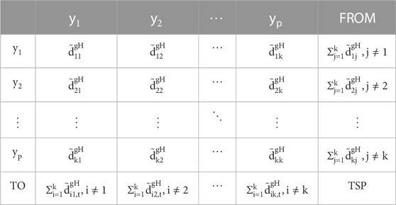
TABLE 2. Global stock market return contagion matrix.
In order to further obtain the time series of the above matrix, we use the rolling window estimation method according to Diebold and Yilmaz [12,13]. First, in order to avoid over-parameterization of the model, we set the VAR to order 1, that is, p = 1. Since we use monthly data, in order to balance the time window and the number of estimated results, we set the rolling window to 50 days. Then, we perform rolling window estimation according to the above method, and let H = 10 estimate the dynamic risk contagion network between global stock markets. Before the estimation of VAR model, this paper has carried out a stationary test on the logarithmic return of each stock market index. The results show that each sequence is a stationary sequence and can be estimated by a VAR model.
4.2 Quantile on quantile regression
4.2.1 Quantile regression model
The traditional linear regression model describes the mean influence of the independent variable on the value of the dependent variable. However, it is difficult to satisfy the assumption that the random disturbance term is identically distributed in real life. Therefore, in the late 1970s, Koenker and Bassett [42] first proposed the standard quantile regression model. They used the conditional quantile of the dependent variable to regress on the independent variable. Therefore, compared with the rough description of the linear model, quantile regression can more accurately describe the influence of the independent variable on different positions of the dependent variable. The model is as follows:
4.2.2 Quantile on quantile regression approach
However, the standard quantile regression model does not account for the effect of different distributions of the independent variables on the dependent variables. Therefore, Sim and Zhou [43] proposed the Quantile-on-Quantile Regression Approach (QQR) in their study regarding the relation between oil and stock returns.
This paper will focus on how global geopolitical risk index impact on the return connectedness between international stock markets under different quantiles of them. To this end, we first propose the linear regression model as follows:
Convert this OLS model into QQ model:
To rewrite
Substitute (17) into (15) and get the following formula:
Eq. 18 represents the
By minimizing Eq. 19, the local linear estimates of
We define
Bandwidth selection is very significant for the kernel function. If the bandwidth is too narrow, the estimation error becomes smaller but the variance increases. If the bandwidth is too large, the estimation variance becomes smaller but the error increases. This paper uses Sim and Zhou [43] bandwidth selection, and selects h = 0.05 in the following empirical process.
5 Empirical results
5.1 Global stock market dynamic contagion network
In this section, we give the relevant estimation results of the global stock market return contagion network.
5.1.1 Global stock price linkage network
Table 3 shows the stock market return connectedness matrix for the full sample. Since we use a rolling window to estimate the data, each window period can generate a market return connectedness matrix. Table 3 shows the mean value of the connectedness matrix
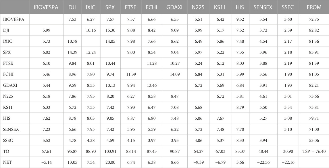
TABLE 3. Global stock market return correlation network.
Table 3 shows that the average TSP of all stock markets is 76.40 percent. This shows that on average, the world’s major stock market indexes exhibit a very high correlation degree. This is a major reason for the transmission of financial market risks to various markets.
Additionally, Table 3 indicates that the Standard & Poor’s 500 Index (SPX), the Dow Jones Industrial Index (DJI), and the German Frankfurt DAX Index (GDAXI) are the three stock market indexes that have the greatest impact on the world. Their impact on global stock market returns is 20%, 13.05% and 8.66%, respectively. The results indicate that North American and European equity markets are leading the way for global equity markets, with other markets following more closely behind. The above results are not surprising. Because the United States is still the world’s largest economy at this stage, its economic strength radiates around the world; and because of the special status of the dollar, the size of the United States stock market and trading volume is still the largest in the world, so the United States stock market has a huge impact on the world economy. As a powerful industry in Europe, Germany’s financial strength, economic strength and political strength are second to none in Europe. The trend of the German stock market can be used as an effective indicator of European economic and financial health.
Finally, from Table 3, we can also find that India‘s Mumbai Sensitive 30 Index (SENSEX), Shanghai Composite Index (SSEC) and Nikkei 225 Index (N225) are the main recipients of global stock market spillover effects, with values of −22.56%, −22.16% and-9.39%, respectively. India and China are the world’s two largest emerging markets, making their stock markets attractive to international investors. There is still a gap between its stock market development and scale and that of developed countries. So, it is more likely to follow the trend of the United States and European stock markets. Japan is the most sought-after haven for global investors except the United States, and the yen is also one of the most valuable reserve currencies. Investors often use the yen and the Japanese stock market for related arbitrage transactions, so Japanese stocks are very vulnerable to other markets.
5.1.2 Dynamic network in the global stock market
In Figure 1, we draw the total international stock market return contagion effect in the rolling sample window. Overall, we can observe three distinct stages. The first phase began in 1995 and ended in early 2009; the second stage lasted from early 2009 to early 2018; the third stage is from 2018 until 2022.
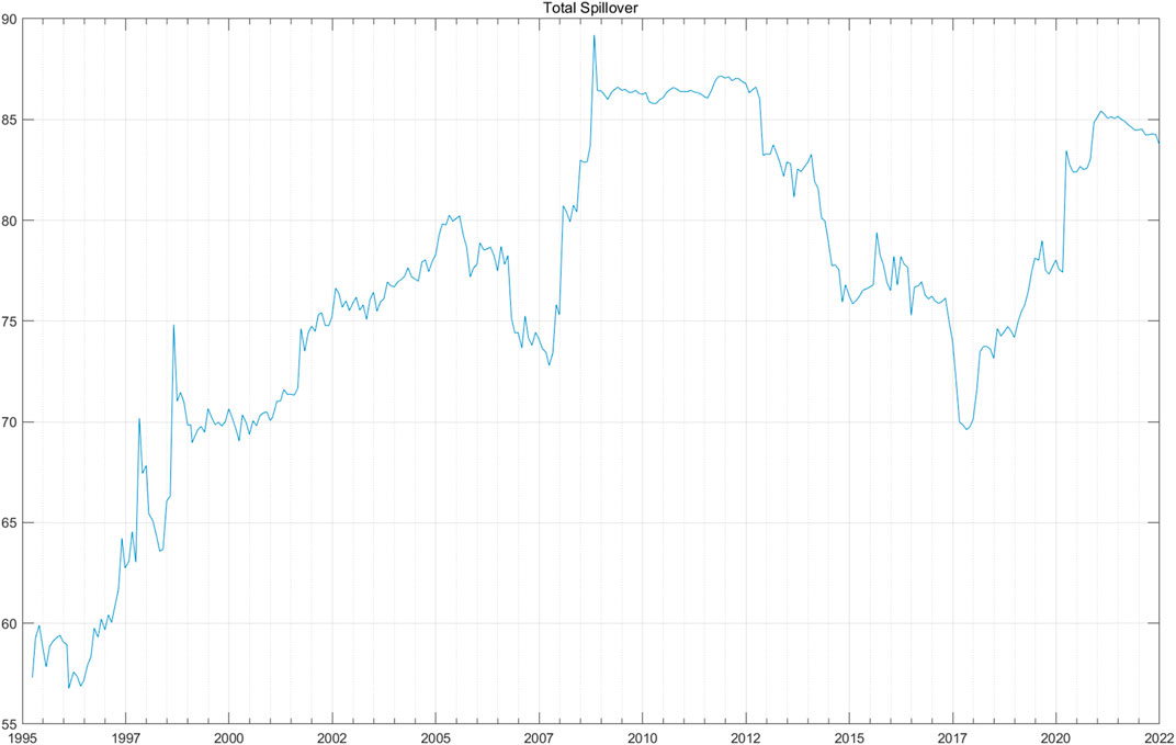
FIGURE 1. Total spillover (TSP).
The first stage coincides with the process of economic globalization around the world. In the process of globalization, most countries in the world have opened up their financial markets, which has greatly increased the linkage between stock prices on various stock markets. The second phase occurred nearly 10 years after the financial crisis. In the 10 years after the financial crisis, governments and investors around the world have absorbed relevant experience. They have carried out strict supervision of capital market openings and derivatives trading. These regulatory measures have reduced the linkage between stock markets in various countries to the level before the crisis. In the third stage, major geopolitical conflicts such as the Sino-US trade war and the Russo-Ukrainian War began to occur frequently. Major risk events not only impact a stock market, but also have a significant impact on the global economy and financial markets. Thus, the price linkage between the various stock markets has been rising in the past 5 years.
Figures 2, 3 show the time series of directional connectedness (“TO” and “FROM”) of each stock market.
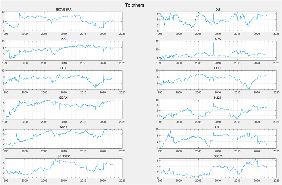
FIGURE 2. To spillover.
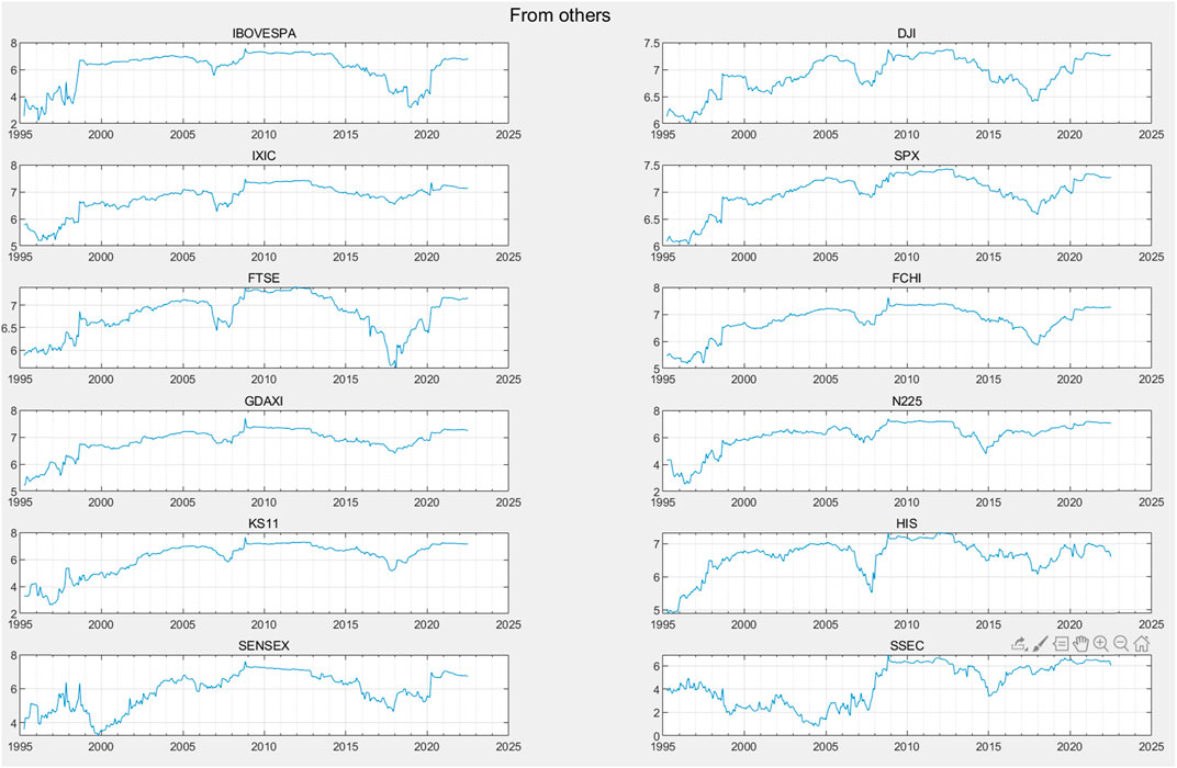
FIGURE 3. From spillover.
From Figure 2, we can see that in the 2008 financial crisis, the “TO” spillover effect of the four stock indexes of DJI, SPX, N225 and FTSE all had an obvious peak, while the “TO” spillover effect of other stock market indexes had no obvious peak. This shows that during the financial crisis, the source of risk was mainly generated by the DJI, SPX, N225, FTSE four indexes. This result is relatively easy to understand, mainly because the US, Japan, and the UK have more active derivatives trading, similar pre-crisis financial regulatory policies, and very high financial dependence. Therefore, when the U. S. subprime mortgage crisis hit, the four indexes had the fastest response. As the crisis deepened, the impact of these four indices slowly spread to other developed and emerging markets.
Another obvious characteristic of Figure 3 is that the change of “FROM” effect is smoother than the change of “TO” effect. This result is consistent with many other studies. This difference is not difficult to explain. When a single stock market index produces an impact, this impact is expected to be transmitted to other stock market indexes. However, when individual stock market indexes receive total impacts from other markets, some fractions of this total impact are very small and can be ignored. Some may be quite large. At this time, the “TO” effect will obviously show more peaks. When a stock market index is hit, one can expect the impact to have a scattered spillover effect on other stock markets. Since each stock market index will be affected by the spillover effects of all other markets, these spillover effects are often smoother after being summed up.
Figure 4 shows the time series diagram of the “NET” index. From Figure 4, we can get a similar conclusion to Table 2. For the most part of the time, the “NET” indicator time series charts of the India Mumbai Sensitivity 30 Index (SENSEX) and the Shanghai Composite Index (SSEC) are below the 0 level. This shows that stock price changes in these two markets are mainly affected by changes in other stock markets. These two indicators have a limited influence on other market indexes. Additionally, the S&P 500 Index (SPX), the Dow Jones Industrial Average (DJI), and the German DAX Index (GDAXI) three “NET” indicator time series diagram is above 0 levels at most of the time, indicating that the world’s stock market index price changes are mostly driven by these three index fluctuations. These results are consistent with the conclusions of Table 2.
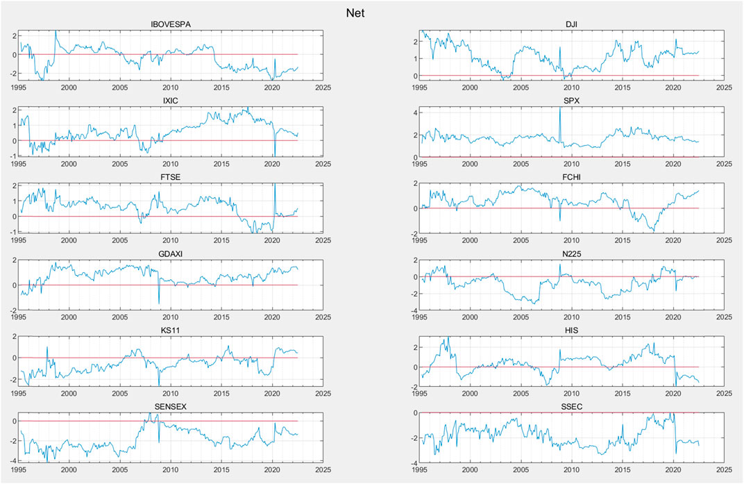
FIGURE 4. Net spillover.
5.2 Global geopolitical risk (GPR) and global stock market total connectedness
Standard quantile regression can estimate the impact of global geopolitical risks on the connectedness of global stock market returns in different states. However, it cannot capture the asymmetric spillover effect of global geopolitical risks on the connectedness of global stock market returns. This ignores the possibility of different states of global geopolitical risks. For example, the impact of global geopolitical risks under high and low risk conditions on the connectedness of global stock market returns may have asymmetric heterogeneity. Therefore, standard quantile regression cannot capture the subtle economic relationship between the two.
The quantile-on-quantile regression model [43] can effectively solve this problem, which characterizes its impact on θ quantile of global stock market connectedness through the τ quantile of global geopolitical risk. Since the estimation coefficients
In this section, we use quantile-on-quantile regression [43] to analyze the impact of global geopolitical risks on the connectedness of the global stock market at different quantiles.
5.2.1 QQR estimation results of intercept for GPR
First, we characterize the intercept influence of global geopolitical risk (GPR) on the connectedness between global stock markets through the intercept term in the formula, namely the estimate of
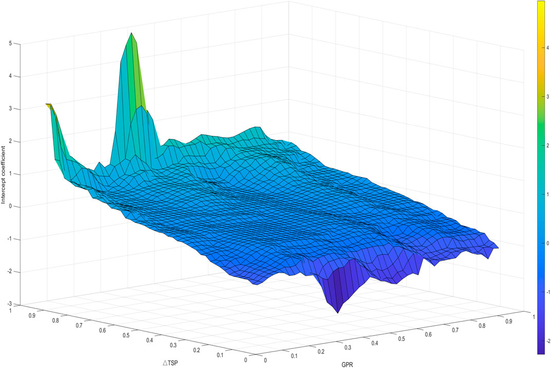
FIGURE 5. QQR estimate of
Figure 5 illustrates the estimated value of
First, in general, this intercept term
Secondly, when
Finally, on the whole, when
5.2.2 QQR estimation results of slope for GPR
In the previous section, we discuss the estimation results of the intercept term of
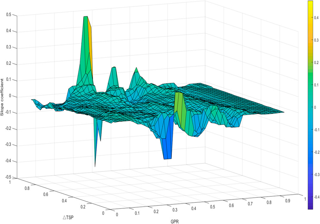
FIGURE 6. QQR estimate of
We can see that Figure 6 is very similar to Figure 5 at the peak. When the global stock market connectedness is at a high quantile, that is, the stock markets are in a state of close interaction, about 0.9–0.95, and the global geopolitical risk is at about 0.35 quantile,
The marginal effect that is completely opposite to this “magnifying glass” effect is called the “reins” effect, which appears in the 0.37–0.40 quantile and 0.49 quantile of GPR. Specifically, when the global stock market correlation is at the low quantile, about 0.05–0.07, the GPR is at the 0.37–0.40 quantile, and the estimated positive value of
However, this difference appears “U-shaped” when the geopolitical risk is around 0.59–0.61, that is, in the case of high and low global market connectedness, the estimated value of
5.3 Global geopolitical action risk (GPRA) and global stock market total connectedness
In this section, we replace the variable of global geopolitical risk (GPR) with the global geopolitical action risk (GPRA). This section focuses on how geopolitical action risk (GPRA) affects the total connectedness of global stock markets.
5.3.1 QQR estimation results of intercept for GPRA
Figure 7 shows the intercept effect of global geopolitical action risks on the connectedness of global stock markets, the estimate of the intercept term
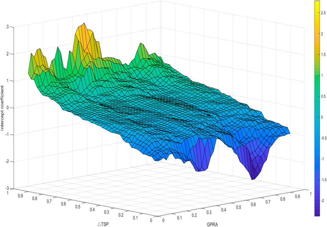
FIGURE 7. QQR estimate of
Figure 7 shows the intercept impact of GPRA on the connectedness of global stock markets, and the results are highly similar to Figure 5. This still represents a change in the intercept influence of GPRA on global stock market correlation from promotion to inhibition when global stock market correlation is close to loose. Based on Figure 7, it can be seen that when the global stock market connectedness is high, i.e., when the
In general, Figure 7 still shows a monotonous change feature, i.e., when the GPRA is at the same quantile, the impact of GPRA on the global stock market connectedness shows a trend from negative to positive.
Reflected in the estimated value of
5.3.2 QQR estimation results of slope for GPRA
In Figure 8, we visualize the marginal effect of the influence of GPRA on the connectedness of global stock markets determined by different
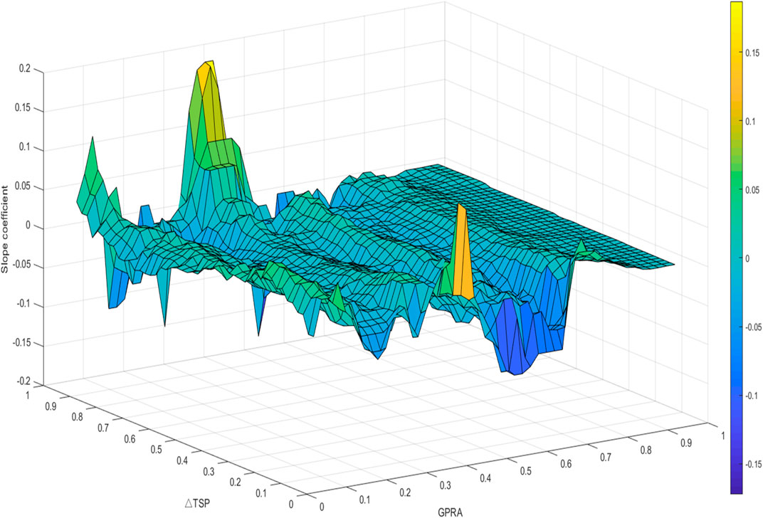
FIGURE 8. QQR estimate of
When compared to the visual Figure 6 of the marginal effect, Figure 8 shows some similarities, but a closer look will reveal a lot of differences. In Figure 6, when the global stock market correlation is at a high level, about 0.91–0.95 quantile, and the GPR is at 0.39 quantile, the marginal effect of the GPR on the global stock market connectedness is estimated to be the minimum valley value. However, in Figure 8, after replacing the GPR with the GPRA, the highest peak value of 0.1869 is estimated under the same quantile conditions. That is to say, under the same quantile conditions, GPR has a negative impact on the global stock market connectedness, and this marginal effect is negative. But, the GPRA has a positive impact on the global stock market connectedness, and the marginal effect is positive. Therefore, it can be seen that after refining the types of geopolitical risks, the impact of geopolitical risks on the connectedness of global stock markets has reached very different conclusions.
Meanwhile, for Figure 8, we can observe several “U-shaped” or “inverted U-shaped” phenomena. When the GPRA is in the 0.37–0.41 quantile, if the global stock market correlation is very close or very loose, the estimated value of
Similar to Figure 6, the risk of local political action is at a high level, that is, 0.89–0.95 of the
5.4 Global geopolitical threat risk (GPRT) and global stock market total connectedness
In this section, we use global geopolitical threat risk (GPRT) to study how geopolitical threat risk affects the connectedness of global stock markets.
5.4.1 QQR estimation results of intercept
First, Figure 9 is a visual image of the estimated value of the intercept term
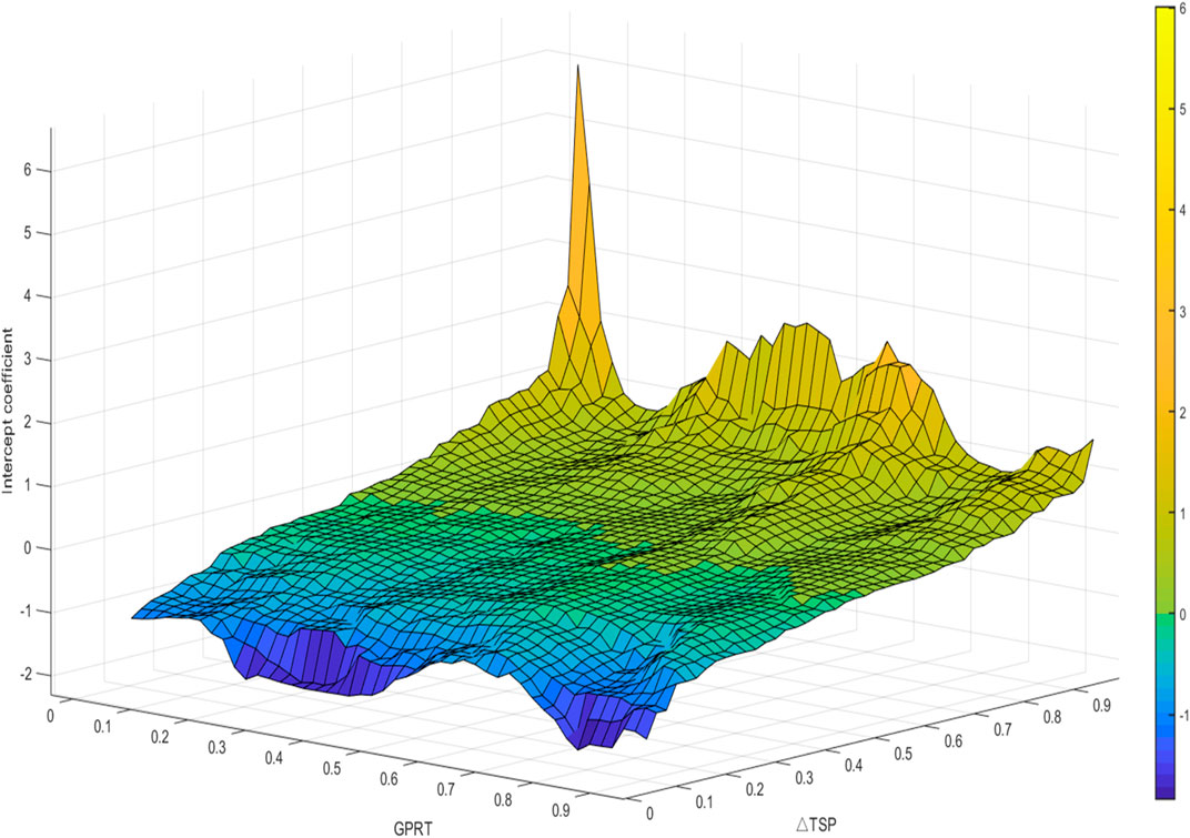
FIGURE 9. QQR estimate of
The most striking thing in Figure 9 is that when the global stock market connectedness is highly correlated (the quantile is at 0.91–0.95), while the GPRT is at a low level (the quantile is 0.05–0.09), the estimated value of marginal effect
On the whole, the estimation results of Figure 9 are similar to those of Figures 5, 7. They all show the monotonic change of the estimated value of
5.4.2 QQR estimation results of slope
Figure 10 describes the marginal effect of GPRT on the connectedness of global stock markets. In Figure 10, the Z-axis still represents the estimated value of the slope term
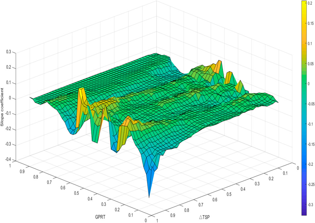
FIGURE 10. QQR estimate of
In Figure 10, when the connectedness level of the global stock market is highly related (
At the same time, the “magnifying glass” effect, the “reins” effect and the “unidirectional” effect in Figures 6, 8 appear in the QQR regression results of Figure 10. The “magnifying glass” effect can be clearly observed in the results of Figure 10. When the GPRT is in the 0.23 quantile, the global stock market is in a highly correlated condition, and the estimated value of
The unidirectional effect in Figure 10 is also very obvious. When the GPRT is at the 0.39 quantile and the global stock market is in a highly related condition, the estimated value of
Similarly, we can also observe the “reins” effect in Figure 10. When the GPRT is at the 0.47 quantile, the estimated value of
Finally, as with other slope estimates, when the GPRT is high, this marginal effect is almost 0 regardless of the global stock market correlation.
6 Conclusion
We use the vector autoregressive regression method (VAR) to construct a global stock market return contagion network, and use the quantile-to-quantile regression (QQR) to investigate the impact of global geopolitical risks on global stock market connectedness.
The main results are summarized as follows:
First, the Indian stock market and the Chinese stock market act as financial shock recipients in the global stock market. For most of the time, the net spillover effects of India’s Mumbai Sensitivity 30 Index (SENSEX) and Shanghai Composite Index (SSEC) are less than 0. Generally, stock prices in these two markets follow those in other markets, and these two markets have not much influence on other market indices. The United States stock market and the German stock market are shock transmitters in the global stock market. The S&P 500 Index (SPX), the Dow Jones Industrial Average (DJI), and the Deutscher Aktien Index (GDAXI) in Germany have net spillover effects over 0. Changes in stock prices in these markets lead to fluctuation in stock prices in other markets. It is not difficult to understand that India and China, as emerging economies, are still in a relatively backward stage of capital market development. In contrast, the United States and Germany have been the world’s leading economies since the economy, occupying an influential position in the global industrial chain and trade chain. At the same time, their capital markets are highly developed, so the asset prices of these two markets have played a role in the vane.
Second, in the quantile-on-quantile regression results between global geopolitical risk (GPR) and the connectedness of global stock market returns, we find that the same level of GPR has a heterogeneous impact on global stock market connectedness under different levels of connectedness. Under the high connectedness of global stock market returns, any quantile of GPR will further consolidate this connectedness; under the low connectedness of global stock market returns, any quantile of GPR will further reduce this correlation.
Third, as GPR quantiles differ, there are two opposite marginal effects: “magnifying glass” and “reins”. The “magnifying glass” effect shows that an increase in GPR will intensify the connectedness of global stock market returns at high quantiles and disintegrate the connectedness of global stock market returns at low quantiles. The “rein” effect indicates that an increase in GPR will reduce the high-quantile global stock market connectedness and increase the low-quantile global stock market connectedness.
Fourth, when we further decompose the global geopolitical risk into GPRA and GPRT, we find that when the global stock market connectedness is not in extreme circumstances, different levels of GPRT will not greatly affect the global stock market’s total connectedness. But when global stock markets are highly correlated and GPRT is at a very low level, any small increase in GPRT would greatly reduce that total connectedness. This phenomenon is also easy to explain. Small stones on the calm water surface will also cause very obvious ripples. In times when the GPRT level is low and global stock market total connectedness is high, any risk problem can break this quiet.
Fifth, when GPRT or GPRA is at high quantiles, their movements will not affect the total connectedness of global stock markets. This phenomenon is contrary to the previous conclusion. When GPRT or GPRA are already at a very high risk level, any further rise will no longer affect global stock market connectedness.
Sixth, we observed several ‘U-shaped’ or ‘inverted U-shaped’ phenomena when we estimated the slope between GPRA and the total connectedness of global stock markets. We call it the " one-way” effect (unidirectional effect), that is, when global stock market total connectedness is in an extreme situation (highly close or highly loose), different levels of GPRA have different marginal effects. Sometimes it increases global stock market total connectedness, and sometimes reduces global stock market total connectedness.
The findings of this study are significant for future research. This helps policymakers and relevant investors to cope with the impact of current high geopolitical risks on the global stock market contagion network. This helps them effectively manage risk in asset allocation and policy formulation. However, there are still some areas where our research can go further. For example, why do these special quantiles have different asymmetric effects? The economic logic and practical significance behind them need to be studied. In addition, research on the volatility contagion network of global stock markets and global geopolitical risks can also be discussed.
Data availability statement
The original contributions presented in the study are included in the article/supplementary materials, further inquiries can be directed to the corresponding author.
Author contributions
FL proposed the conceptualization and methodology, performed the coding and data analysis. SL performed original draft, data analysis; and gave formal writing—review and editing. LL performed the data collection and original data arrangement. SZ performed the funding acquisition, original draft preparation, data analysis and data preparation; modified final draft.
Funding
This study was supported by Yunnan Fundamental Research Projects (grant No. 202201AU070101), Scientific Research Foundation of Yunnan University of Finance and Economics (No. 2021D07), The Ministry of Education of Humanities and Social Science project (No. 22XJCZH007), Scientific Research Fund Project of Yunnan Education Department (No. 2021J0586).
Conflict of interest
The authors declare that the research was conducted in the absence of any commercial or financial relationships that could be construed as a potential conflict of interest.
Publisher’s note
All claims expressed in this article are solely those of the authors and do not necessarily represent those of their affiliated organizations, or those of the publisher, the editors and the reviewers. Any product that may be evaluated in this article, or claim that may be made by its manufacturer, is not guaranteed or endorsed by the publisher.
References
1. Bohl D, Hanna T, Mapes BR, Moyer JD, Narayan K, Wasif K. Understanding and forecasting geopolitical risk and benefits. SSRN J (2017). doi:10.2139/ssrn.3941439
2. Caldara D, Iacoviello M. Measuring geopolitical risk. Am Econ Rev (2022) 112:1194–225. doi:10.1257/aer.20191823
3. Balcilar M, Bonato M, Demirer R, Gupta R. Geopolitical risks and stock market dynamics of the BRICS. Econ Syst (2018) 42:295–306. doi:10.1016/j.ecosys.2017.05.008
4. Cheng S, Han L, Cao Y, Jiang Q, Liang R. Gold-oil dynamic relationship and the asymmetric role of geopolitical risks: Evidence from Bayesian pdBEKK-GARCH with regime switching. Resour Pol (2022) 78:102917. doi:10.1016/j.resourpol.2022.102917
5. Huang J, Ding Q, Zhang H, Guo Y, Suleman MT. Nonlinear dynamic correlation between geopolitical risk and oil prices: A study based on high-frequency data. Res Int Business Finance (2021) 56:101370. doi:10.1016/j.ribaf.2020.101370
6. Ivanovski K, Hailemariam A. Time-varying geopolitical risk and oil prices. Int Rev Econ Finance (2022) 77:206–21. doi:10.1016/j.iref.2021.10.001
7. Kumar S, Khalfaoui R, Tiwari AK. Does geopolitical risk improve the directional predictability from oil to stock returns? Evidence from oil-exporting and oil-importing countries. Resour Pol (2021) 74:102253. doi:10.1016/j.resourpol.2021.102253
8. Li S, Tu D, Zeng Y, Gong C, Yuan D. Does geopolitical risk matter in crude oil and stock markets? Evidence from disaggregated data. Energ Econ (2022) 113:106191. doi:10.1016/j.eneco.2022.106191
9. Long H, Demir E, Będowska-Sójka B, Zaremba A, Shahzad SJH. Is geopolitical risk priced in the cross-section of cryptocurrency returns? Finance Res Lett (2022) 49:103131. doi:10.1016/j.frl.2022.103131
10. Sohag K, Hammoudeh S, Elsayed AH, Mariev O, Safonova Y. Do geopolitical events transmit opportunity or threat to green markets? Decomposed measures of geopolitical risks. Energ Econ (2022) 111:106068. doi:10.1016/j.eneco.2022.106068
11. Su CW, Khan K, Umar M, Zhang W. Does renewable energy redefine geopolitical risks? Energy Policy (2021) 158:112566. doi:10.1016/j.enpol.2021.112566
12. Diebold FX, Yilmaz K. Better to give than to receive: Predictive directional measurement of volatility spillovers. Int J Forecast (2012) 28:57–66. doi:10.1016/j.ijforecast.2011.02.006
13. Diebold FX, Yılmaz K. On the network topology of variance decompositions: Measuring the connectedness of financial firms. J Econom (2014) 182:119–34. doi:10.1016/j.jeconom.2014.04.012
14. Cunado J, Gupta R, Lau CKM, Sheng X. Time-varying impact of geopolitical risks on oil prices. Defence Peace Econ (2020) 31:692–706. doi:10.1080/10242694.2018.1563854
15. Mei D, Ma F, Liao Y, Wang L. Geopolitical risk uncertainty and oil future volatility: Evidence from MIDAS models. Energ Econ (2020) 86:104624. doi:10.1016/j.eneco.2019.104624
16. Abdel-Latif H, El-Gamal M. Financial liquidity, geopolitics, and oil prices. Energ Econ (2020) 87:104482. doi:10.1016/j.eneco.2019.104482
17. Su CW, Qin M, Tao R, Moldovan NC. Is oil political? From the perspective of geopolitical risk. Defence Peace Econ (2021) 32:451–67. doi:10.1080/10242694.2019.1708562
18. Demirer R, Gupta R, Suleman T, Wohar ME. Time-varying rare disaster risks, oil returns and volatility. Energ Econ (2018) 75:239–48. doi:10.1016/j.eneco.2018.08.021
19. Liu J, Ma F, Tang Y, Zhang Y. Geopolitical risk and oil volatility: A new insight. Energ Econ (2019) 84:104548. doi:10.1016/j.eneco.2019.104548
20. Sharif A, Aloui C, Yarovaya L. COVID-19 pandemic, oil prices, stock market, geopolitical risk and policy uncertainty nexus in the US economy: Fresh evidence from the wavelet-based approach. Int Rev Financial Anal (2020) 70:101496. doi:10.1016/j.irfa.2020.101496
21. Antonakakis N, Gupta R, Kollias C, Papadamou S. Geopolitical risks and the oil-stock nexus over 1899–2016. Finance Res Lett (2017) 23:165–73. doi:10.1016/j.frl.2017.07.017
22. Diks C, Wolski M. Nonlinear granger causality: Guidelines for multivariate analysis: Multivariate nonlinear granger causality. J Appl Econ (2016) 31:1333–51. doi:10.1002/jae.2495
23. Hoque ME, Soo Wah L, Zaidi MAS. Oil price shocks, global economic policy uncertainty, geopolitical risk, and stock price in Malaysia: Factor augmented VAR approach. Econ Research-Ekonomska Istraživanja (2019) 32:3700–32. doi:10.1080/1331677X.2019.1675078
24. Smales LA. Geopolitical risk and volatility spillovers in oil and stock markets. Q Rev Econ Finance (2021) 80:358–66. doi:10.1016/j.qref.2021.03.008
25. Su CW, Khan K, Tao R, Nicoleta-Claudia M. Does geopolitical risk strengthen or depress oil prices and financial liquidity? Evidence from Saudi arabia. Energy (2019) 187:116003. doi:10.1016/j.energy.2019.116003
26. Abadie A, Gardeazabal J. The economic costs of conflict: A case study of the Basque country. Am Econ Rev (2003) 93:113–32. doi:10.1257/000282803321455188
27. Blomberg B, Hess G, Jackson JH. Terrorism and the returns to oil. Econ Polit (2009) 21:409–32. doi:10.1111/j.1468-0343.2009.00357.x
28. Kollias C, Kyrtsou C, Papadamou S. The effects of terrorism and war on the oil price–stock index relationship. Energ Econ (2013) 40:743–52. doi:10.1016/j.eneco.2013.09.006
29. Orbaneja JRV, Iyer SR, Simkins BJ. Terrorism and oil markets: A cross-sectional evaluation. Finance Res Lett (2018) 24:42–8. doi:10.1016/j.frl.2017.06.016
30. Toft P, Duero A, Bieliauskas A. Terrorist targeting and energy security. Energy Policy (2010) 38:4411–21. doi:10.1016/j.enpol.2010.03.070
31. Hoque ME, Zaidi MAS. Global and country-specific geopolitical risk uncertainty and stock return of fragile emerging economies. Borsa Istanbul Rev (2020) 20:197–213. doi:10.1016/j.bir.2020.05.001
32. Apergis N, Bonato M, Gupta R, Kyei C. Does geopolitical risks predict stock returns and volatility of leading defense companies? Evidence from a nonparametric approach. Defence Peace Econ (2017) 2017:1–13. doi:10.1080/10242694.2017.1292097
33. Yang J, Yang C. The impact of mixed-frequency geopolitical risk on stock market returns. Econ Anal Pol (2021) 72:226–40. doi:10.1016/j.eap.2021.08.008
34. Salisu AA, Ogbonna AE, Lasisi L, Olaniran A. Geopolitical risk and stock market volatility in emerging markets: A GARCH – MIDAS approach. North Am J Econ Finance (2022) 62:101755. doi:10.1016/j.najef.2022.101755
35. Zhang Y, Hamori S. A connectedness analysis among BRICS’s geopolitical risks and the US macroeconomy. Econ Anal Pol (2022) 76:182–203. doi:10.1016/j.eap.2022.08.004
36. Baker SR, Bloom N, Davis SJ. Measuring economic policy uncertainty. Q J Econ (2016) 131:1593–636. doi:10.1093/qje/qjw024
37. Das D, Kannadhasan M, Bhattacharyya M. Do the emerging stock markets react to international economic policy uncertainty, geopolitical risk and financial stress alike? North Am J Econ Finance (2019) 48:1–19. doi:10.1016/j.najef.2019.01.008
38. Saiz A, Simonsohn U. Proxying for unobservable variables with internet document-frequency. J Eur Econ Assoc (2013) 11:137–65. doi:10.1111/j.1542-4774.2012.01110.x
39. Kotcharin S, Maneenop S. Geopolitical risk and corporate cash holdings in the shipping industry. Transportation Res E: Logistics Transportation Rev (2020) 136:101862. doi:10.1016/j.tre.2020.101862
40. Le A-T, Tran TP. Does geopolitical risk matter for corporate investment? Evidence from emerging countries in Asia. J Multinational Financial Manage (2021) 62:100703. doi:10.1016/j.mulfin.2021.100703
41. Wang KH, Xiong DP, Mirza N, Shao XF, Yue XG. Does geopolitical risk uncertainty strengthen or depress cash holdings of oil enterprises? Evidence from China. Pacific-Basin Finance J (2021) 66:101516. doi:10.1016/j.pacfin.2021.101516
Keywords: global geopolitical risks, contagion network, connectedness, quantile-on-quantile regression, stock market
Citation: Lai F, Li S, Lv L and Zhu S (2023) Do global geopolitical risks affect connectedness of global stock market contagion network? Evidence from quantile-on-quantile regression. Front. Phys. 11:1124092. doi: 10.3389/fphy.2023.1124092
Received: 14 December 2022; Accepted: 27 February 2023;
Published: 10 March 2023.
Edited by:
Jianbo Wang, Southwest Petroleum University, ChinaReviewed by:
Shaoping Li, Huzhou University, ChinaWang Tao, University of Southern California, United States
Copyright © 2023 Lai, Li, Lv and Zhu. This is an open-access article distributed under the terms of the Creative Commons Attribution License (CC BY). The use, distribution or reproduction in other forums is permitted, provided the original author(s) and the copyright owner(s) are credited and that the original publication in this journal is cited, in accordance with accepted academic practice. No use, distribution or reproduction is permitted which does not comply with these terms.
*Correspondence: Sha Zhu, emh1c2hhY3VmZUAxNjMuY29t