An investigation of a closed-form solution for non-linear variable-order fractional evolution equations via the fractional Caputo derivative

Determining the non-linear traveling or soliton wave solutions for variable-order fractional evolution equations (VO-FEEs) is very challenging and important tasks in recent research fields. This study aims to discuss the non-linear space–time variable-order fractional shallow water wave equation that represents non-linear dispersive waves in the shallow water channel by using the Khater method in the Caputo fractional derivative (CFD) sense. The transformation equation can be used to get the non-linear integer-order ordinary differential equation (ODE) from the proposed equation. Also, new exact solutions as kink- and periodic-type solutions for non-linear space–time variable-order fractional shallow water wave equations were constructed. This confirms that the non-linear fractional variable-order evolution equations are natural and very attractive in mathematical physics.

1 Introduction

Fractional calculus is a generalization of traditional integer-order integration and derivation actions onto non-integer order. The idea of fractional calculus is as old as classical calculus; it was discussed for the first time by Leibniz and L’Hospital in 1965. The fractional- and variable-order VO fractional models gained more attention because these models describe the physical phenomenon properly as compared to integer-order differential models. The non-linear FEEs define different phenomena in various areas, such as signal preparation, medication, biology, and organic framework [1, 2]. Many strategies have been produced to solve integer/fractional-order problems. Various fractional-order literature works directed that the memory and/or non-locality of the system may change with time, space, or other conditions. So, here our focus is on VO fractional differential models, which describe the physical models that vary with time or space or space–time. For example, Akgül et al. [3] solved the VO FPDE numerically and presented numerical experiments to confirm the efficiency and feasibility. Katsikadelis [4] developed a numerical method for linear and non-linear VO FPDEs in the Caputo sense. The resultant numerical values demonstrated the accuracy of the proposed method. Sahoo et al. [5] reviewed the VO operator definitions and properties. They discussed the new transfer function and investigated the model of a dynamic viscoelastic oscillator. Sing et al. [6] suggested an SEIR model that modeled the 2014–2015 outbreak of the Ebola virus in Africa. They discussed the system of VO FDEs and estimated its parameters for one or more variables. Semary et al. [7] approximated the solution of Liouville–Caputo VO FPDEs with $0<\alpha \left(t\right)\le 1$ based on the Chebyshev function and discussed many linear and non-linear non-integer-order PDEs. Taghipour and Aminikhah [8] proposed the ADI numerical scheme for the fractional-order model and discussed the theoretical analysis. Other related studies can be seen in [9–16]. The effective analytical and closed-form solutions are studied in the recent literature. For example, Uddin et al. [17] considered the two important fractional-order models, namely, equal width and generalized equal width that describe the dispersive waves. They used the fractional derivative in the Riemann–Liouville sense and the $\left(\frac{G^{\prime }}{G},\frac{1}{G}\right)$ expansion approach has been used, and they confirmed that the proposed approach is powerful, very convenient, and computationally efficient. Barman et al. [18] worked on a generalized Kudryashov method to provide a generic and inclusive closed-form solution. The proposed approach confirmed various shapes of waveform solutions such as kink-shaped, bell-shaped, singular, and flat in a 3D form. In another study, Barman et al. [19] proposed the same technique for Konopelchenko–Dubrovsky and Landau–Ginzburg–Higgs models. They obtained various varieties of analytical solutions for different parameters. The solutions are obtained in 2D and 3D forms, which demonstrated the efficiency and reliability of the proposed method. Roy et al. [20] solved the two significant types of models and implemented the new generalized $G^{\prime }/G$ expansion method. They constructed the solution in trigonometric, hyperbolic, and rational forms with different parameters. Kumar et al. [21] found out the exact solution for the higher-dimensional Fokas and breaking soliton models by the generalized exponential function method. The authors observed that the suggested method is effective and powerful. Ali et al. [22] investigated the exact solution for the VO fractional modified equal width equation based on the exp $\left(-\varphi \left(\xi \right)\right)$ method. The fractional derivative is obtained in the Caputo sense, and the obtained exact solution is new and somewhat natural in mathematical physics. Akhtar et al. [23] constructed exact and traveling wave solutions for the Konopelchenko–Dubrovsky model and used two types of integration schemes. The resultant solutions are dark, single, anti-kink forms having a wide range of applications in applied sciences. Islam et al. [24] worked on analytical techniques and found the solution for the fractional-order foam drainage equation and SRLW equation. They used the $G^{\prime }/G$ expansion method and investigated the traveling wave solution for the proposed models. Mamun et al. [25] discussed the double $\left(\frac{G^{\prime }}{G},\frac{1}{G}\right)$ expansion approach for the breaking soliton and the (1 + 1)-dimensional classical Boussinesq equations and obtained different soliton solutions, such as kink, multi-periodic, single soliton, and periodic wave solutions for different values of parameters. The comprehensive study can be found in [26–35].

The aforementioned cited literature reported that so far only numerical studies have been discussed for VO models and no attempt has been made to find the closed form for such types of VO-FEEs. The objective of this paper is to discuss the closed-form solution of the non-linear VO-FEEs. Here, we solve the non-linear VO fractional shallow water wave equation with CFD using the Khater method. The VO fractional problems are more complex computationally than a constant fractional order, and the evolution of a system can be furthermore clearly and accurately described. This contribution seems natural and simple and models many systems with VO [36]. The traveling wave solutions for the VO physical models are not known to the authors.

2 The outline of the Khater method

The non-linear variable-order $\alpha \left(x,y,\dots ,t\right)$ FPDE is given as

$\mathrm{H}\left(D_x^{\alpha \left(x,y,..,t\right)}Y,{D_x^{\alpha \left(x,y,..,t\right)}D}_t^{\alpha \left(x,y,..,t\right)}Y,D_x^{\alpha \left(x,y,..,t\right)}{D}_y^{2\alpha \left(x,y,..,t\right)}Y,\dots \right)=0.(1)$

where $H$ is a polynomial for $Y,Y_t,Y_x,D_t^{\alpha \left(x,y,..,t\right)},D_x^{\alpha \left(x,y,..,t\right)},D_y^{\alpha \left(x,y,..,t\right)}$ and $D^{\alpha \left(x,y,..,t\right)}$ represents Caputo fractional derivatives of the variable-order $\alpha \left(x,y,...,t\right)$. The Caputo fractional derivative of the variable order for a function $Y\left(x,t\right)$ of order $\left.\gamma (x,t)ϵ(0,1\right]$ is defined as follows [22]:

$D_t^{\gamma \left(x,t\right)}Y\left(x,t\right)=\left\{\begin{array}{l}\frac{1}{\mathrm{\Gamma }\left(1+\gamma \left(x,t\right)\right)}{\int }_0^t\frac{Y^{\prime }\left(x,t\right)}{\mathrm{\Gamma }{\left(t-\xi \right)}^{\gamma \left(x,t\right)}}d\xi ,0<\gamma \left(x,t\right)<1,\\ Y^{\prime }\left(x,t\right),\gamma \left(x,t\right)=1.\end{array}\right.(2)$

Also, the important property is given as follows:

${\mathit{D}}_{\mathit{t}}^{\mathit{\gamma }\left(\mathit{x},\mathit{t}\right)}{\mathit{t}}^{\mathit{\beta }}=\frac{\mathrm{\Gamma }\left(1-\mathit{\beta }\right)}{\mathrm{\Gamma }\left(1-\mathit{\beta }+\mathit{\gamma }\left(\mathit{x},\mathit{t}\right)\right)}{\mathit{t}}^{\mathit{\beta }-\mathit{\gamma }\left(\mathit{x},\mathit{t}\right)},0<\mathit{\gamma }\left(\mathit{x},\mathit{t}\right)<1.(3)$

Eq. 1 involved the linear and non-linear highest-order derivatives. A brief explanation of the proposed method is as follows [37]:

Convert the variable-order FPDE into an ordinary differential equation (ODE) by taking the transformation as

$Y\left(x,y,t\right)=y\left(\xi \right),\xi =\frac{k{x}^{\alpha \left(x,y,..,t\right)}}{\mathrm{\Gamma }\left(1+\alpha \left(x,y,..,t\right)\right)}+\frac{l{y}^{\alpha \left(x,y,..,t\right)}}{\mathrm{\Gamma }\left(1+\alpha \left(x,y,..,t\right)\right)}+\cdots -\frac{\omega t^{\alpha \left(x,y,..,t\right)}}{\mathrm{\Gamma }\left(1+\alpha \left(x,y,..,t\right)\right)}.(4)$

The obtained ODE is as follows:

$\mathrm{H}\left(y,\omega y^{\prime },k{y}^{″},l{y}^{‴},\omega l{y}^{‴},kl{y}^{‴},\dots \right)=0,(5)$

where $k,l,m,$ and $\omega$ are constant parameters, if necessary, integrate Eq. 5. Next, we constructed a trial solution which can be expressed as

$y\left(\xi \right)=\sum _{n=0}^M{a}_n{a}^{nf\left(\xi \right)},(6)$

where $a_n\left(n=1,2,\dots ,M-1\right)$ can be zero and $a_M\ne 0$, and the function $f\left(\xi \right)$ satisfies the following second-order linear equation:

$f^{\prime }\left(\xi \right)=\frac{1}{\ln \left(a\right)}\left(\alpha a^{-f\left(\xi \right)}+\beta +\sigma a^{f\left(\xi \right)}\right).(7)$

The aforementioned equation has 27 possible solutions [33], which are derived by formulating various traveling wave solutions. Furthermore, the balancing principle is used to find $M$. Substituting Eq. 6 in Eq. 5 and Eq. 7, an equation involving the term $\left(a^{f\left(\xi \right)}\right)$ is obtained. In the obtained system of equations, the same power of $\left(a^{f\left(\xi \right)}\right)$ is equated to zero. The equations are solved simultaneously to find all unknown constants.

The solutions to Eq. 7:

When ${\beta }^2-4\alpha \sigma <0$ and $\sigma \ne 0$,

$a^{f\left(\xi \right)}=\frac{-\beta +\sqrt{4\alpha \sigma -{\beta }^2}\tan \left(\frac{\sqrt{4\alpha \sigma -{\beta }^2}}{2}\xi \right)}{2\sigma }(8)$

or

$a^{f\left(\xi \right)}=\frac{-\beta -\sqrt{4\alpha \sigma -{\beta }^2}\cot \left(\frac{\sqrt{4\alpha \sigma -{\beta }^2}}{2}\xi \right)}{2\sigma }.(9)$

When ${\beta }^2-4\alpha \sigma >0$ and $\sigma \ne 0$,

$a^{f\left(\xi \right)}=\frac{-\beta -\sqrt{{\beta }^2-4\alpha \sigma }\tanh \left(\frac{\sqrt{{\beta }^2-4\alpha \sigma }}{2}\xi \right)}{2\sigma }(10)$

or

$a^{f\left(\xi \right)}=\frac{-\beta -\sqrt{{\beta }^2-4\alpha \sigma }\coth \left(\frac{\sqrt{{\beta }^2-4\alpha \sigma }}{2}\xi \right)}{2\sigma }.(11)$

When ${\beta }^2+4{\alpha }^2<0$, $\mathrm{\sigma }\ne 0$, and $\sigma =-p$,

$a^{f\left(\xi \right)}=\frac{\beta -\sqrt{-\left({\beta }^2+4{\alpha }^2\right)}\tan \left(\frac{\sqrt{-\left({\beta }^2+4{\alpha }^2\right)}}{2}\xi \right)}{2\alpha }(12)$

or

$a^{f\left(\xi \right)}=\frac{+\beta \sqrt{-\left({\beta }^2+4{\alpha }^2\right)}\mathit{cot}\left(\frac{\sqrt{-\left({\beta }^2+4{\alpha }^2\right)}}{2}\xi \right)}{2\alpha }.(13)$

When ${\beta }^2+4{\alpha }^2>0$, $\sigma \ne 0$, and $\sigma =-\alpha$,

$a^{f\left(\xi \right)}=\frac{\beta +\sqrt{\left({\beta }^2+4{\alpha }^2\right)}\tanh \left(\frac{\sqrt{\left(q^2+4p^2\right)}}{2}\xi \right)}{2\alpha }(14)$

or

$a^{f\left(\xi \right)}=\frac{\beta +\sqrt{\left({\beta }^2+4{\alpha }^2\right)}\coth \left(\frac{\sqrt{\left({\beta }^2+4{\alpha }^2\right)}}{2}\xi \right)}{2\alpha }.(15)$

When ${\beta }^2-4{\alpha }^2<0$ and $\sigma =\alpha$,

$a^{f\left(\xi \right)}=\frac{-\beta +\sqrt{-\left({\beta }^2-4{\alpha }^2\right)}\tanh \left(\frac{\sqrt{-\left(q^2-4p^2\right)}}{2}\xi \right)}{2\alpha }(16)$

or

$a^{f\left(\xi \right)}=\frac{-\beta -\sqrt{-\left({\beta }^2-4{\alpha }^2\right)}\coth \left(\frac{\sqrt{-\left({\beta }^2-4{\alpha }^2\right)}}{2}\xi \right)}{2\alpha }.(17)$

When ${\beta }^2-4{\alpha }^2>0$ and $\sigma =\alpha$,

$a^{f\left(\xi \right)}=\frac{-\beta -\sqrt{\left({\beta }^2-4{\alpha }^2\right)}\tanh \left(\frac{\sqrt{\left({\beta }^2-4{\alpha }^2\right)}}{2}\xi \right)}{2\alpha }(18)$

or

$a^{f\left(\xi \right)}=\frac{-\beta -\sqrt{{\beta }^2-4{\alpha }^2}\mathit{cot}h\left(\frac{\sqrt{{\beta }^2-4{\alpha }^2}}{2}\xi \right)}{2\alpha }.(19)$

When ${\beta }^2=4\alpha \sigma$,

$a^{f\left(\xi \right)}=-\frac{2+\beta \xi }{2\sigma \xi }.(20)$

When $\sigma \alpha <0$, $\beta =0$, and $\sigma \ne 0$,

$a^{f\left(\xi \right)}=-\sqrt{\frac{-\alpha }{\sigma }}\tanh \left(\sqrt{-\sigma \alpha }\xi \right)(21)$

or

$a^{f\left(\xi \right)}=-\sqrt{\frac{-\alpha }{\sigma }}\mathit{cot}\mathrm{h}\left(\sqrt{-\sigma \alpha }\xi \right).(22)$

When $\beta =0$ and $\alpha =-\sigma$,

$a^{f\left(\xi \right)}=\frac{1+e^{\left(-2\sigma \xi \right)}}{-1+e^{\left(-2\sigma \xi \right)}}.(23)$

When $\alpha =\sigma =0$,

$a^{f\left(\xi \right)}=\cosh \left(\beta \xi \right)+\sinh \left(\beta \xi \right).(24)$

When $\alpha =\beta =k$ and $\sigma =0$,

$a^{f\left(\xi \right)}=e^{k\xi }-1.(25)$

When $\beta =\sigma =k$ and $\alpha =0$,

$a^{f\left(\xi \right)}=\frac{e^{k\xi }}{1-e^{k\xi }}.(26)$

When $\beta =\alpha +\sigma$,

$a^{f\left(\xi \right)}=-\frac{1-\alpha e^{\left(\alpha -\sigma \right)\xi }}{1-\sigma e^{\left(\alpha -\sigma \xi \right)}}.(27)$

When $\beta =-\left(\alpha +\sigma \right)$,

$a^{f\left(\xi \right)}=\frac{\alpha -e^{\left(\alpha -\sigma \right)\xi }}{\sigma -e^{\left(\alpha -\sigma \right)\xi }}.(28)$

When $\alpha =0$,

$a^{f\left(\xi \right)}=\frac{\beta e^{\beta \xi }}{1-\sigma e^{\beta \xi }}.(29)$

When $\sigma =\beta =\alpha \ne 0$,

$a^{f\left(\xi \right)}=\frac{1}{2}\left\{\sqrt{3}\mathit{tan}\left(\frac{\sqrt{3}}{2}\alpha \xi \right)-1\right\}.(30)$

When $\sigma =\beta =0$,

$a^{f\left(\xi \right)}=\alpha \xi .(31)$

When $\alpha =\beta =0$,

$a^{f\left(\xi \right)}=\frac{-1}{\sigma \xi }.(32)$

When $\sigma =\alpha$ and $\beta =0$,

$a^{f\left(\xi \right)}=\tan \left(\alpha \xi \right).(33)$

When $\sigma =0$,

$a^{f\left(\xi \right)}=e^{\beta \xi }-\frac{\alpha }{\beta }.(34)$

The exact solutions for Eq. 1 are obtained by substituting unknown constants and Eq. 7 in Eq. 6.

3 Formulation for the solutions of shallow water wave equations

Shallow water waves arise in the ocean when the waves move from the center of the ocean to the shore or beach known as shallow water waves. Most of the ocean waves are produced by wind, tsunamis, earthquakes, tides, etc. [38], which carry energy. Tsunamis and tides are both shallow water waves. The shallow water wave equation has been derived from the Navier–Stokes equations. Here, we apply the proposed method to study the non-linear space–time fractional VO shallow water wave equation and construct a traveling wave solution based on the Khater method.

3.1 The non-linear space–time variable-order fractional shallow water wave equation

We consider the space–time VO fractional shallow water wave equation as follows [39]:

$D_t^{2\gamma \left(x,t\right)}\left(D_x^{\delta \left(x,t\right)}Y\right)+3D_x^{\delta \left(x,t\right)}Y{D}_t^{\delta \left(x,t\right)}Y-D_x^{\delta \left(x,t\right)}Y-D_t^{\gamma \left(x,t\right)}Y=0.(35)$

Using the wave variable $\xi =\frac{k{x}^{\delta \left(x,t\right)}}{\mathrm{\Gamma }\left(1+\delta \left(x,t\right)\right)}-\frac{\omega t^{\gamma \left(x,t\right)}}{\mathrm{\Gamma }\left(1+\gamma \left(x,t\right)\right)}$, Eq. 35 simplified to

$k{\omega }^2{y}^{‴}-3k\omega {\left(y^{\prime }\right)}^2-k{y}^{\prime }+\omega y^{\prime }=0.(36)$

By balancing the highest-order non-linear term ${\left(y^{\prime }\right)}^2$ and the highest-order linear term $y^{‴}$, we obtain $M=1.$ Therefore, the solution of Eq. 6 becomes

$y=a_0+a_1{a}^{f\left(\xi \right)}.(37)$

Substituting Eq. 37 into Eq. 36 yields a polynomial equation for $\left(a^{f\left(\xi \right)}\right).$ Equating the like powers of ${\left(a^{f\left(\xi \right)}\right)}^n$, we attain a system of algebraic equations given as

${\left(a^{f\left(\xi \right)}\right)}^0:2{\alpha }^{2}k{\omega }^2\sigma a_1^2-3{\alpha }^{2}k\omega a_1^4+\alpha {\beta }^{2}k{\omega }^2{a}_1^2-\alpha k{a}_1^2+\alpha \omega a_1^2=0,$

${\left(a^{f\left(\xi \right)}\right)}^1:8\alpha \beta k{\omega }^2{a}_1^2-6\alpha \beta k\omega a_1^4+{\beta }^{3}k{\omega }^2{a}_1^2-\beta k{a}_1^2+\beta \omega a_1^2=0,$

${\left(a^{f\left(\xi \right)}\right)}^2:8\alpha k{\omega }^2{\sigma }^2{a}_1^2-6\alpha k\omega a_1^4+7{\beta }^{2}k\omega a_1^4-k\sigma a_1^2+\omega \sigma a_1^2=0,$

${\left(a^{f\left(\xi \right)}\right)}^3:12\beta k{\omega }^2{\sigma }^2{a}_1^2-6\alpha \beta k\omega a_1^4=0,$

${\left(a^{f\left(\xi \right)}\right)}^4:6k{\omega }^2{\sigma }^3{a}_1^2-3k\omega {\sigma }^2{a}_1^4=0.$

Solving the aforementioned system of algebraic equations by using computer algebra, we obtain

$\mathbf{S}\mathbf{e}\mathbf{t}\mathbf{1}:a_0=a_0,a_1=\sqrt{\frac{\left(1+\sqrt{1-16\alpha k^2\sigma +4{\beta }^2{k}^2}\right)\sigma }{\left(4\alpha \sigma -{\beta }^2\right)k}},\omega =\frac{1+\sqrt{1-16\alpha k^2\sigma +4{\beta }^2{k}^2}}{2\left(4\alpha \sigma -{\beta }^2\right)k},(38)$

where $\omega ,k,\alpha ,\beta$, and $\sigma$ are arbitrary constants.

Substituting Eq. 38 into Eq. 37, we obtain

$y_1=a_0+\sqrt{\frac{\left(1+\sqrt{1-16\alpha k^2\sigma +4{\beta }^2{k}^2}\right)\sigma }{\left(4\alpha \sigma -{\beta }^2\right)k}}{a}^{f\left(\xi \right)}.(39)$

Now, substituting the solutions of Eq. 7, we obtain the following 27 distinct traveling wave solutions for space–time fractional variable-order shallow water wave Eq. 35:

When ${\beta }^2-4\alpha \sigma <0$ and $\sigma \ne 0$,

$Y_1=\frac{\left(\sqrt{4\alpha \sigma -{\beta }^2}\tan \left(\frac{1}{2}\sqrt{4\alpha \sigma -{\beta }^2}\left(\frac{k{x}^{\delta \left(x,t\right)}}{\mathrm{\Gamma }\left(1+\delta \left(x,t\right)\right)}-\frac{\omega t^{\gamma \left(x,t\right)}}{\mathrm{\Gamma }\left(1+\gamma \left(x,t\right)\right)}\right)\right)-\beta \right)\sqrt{-\frac{\left(1+\sqrt{1-16\alpha k^2\sigma +4{\beta }^2{k}^2}\right)\sigma }{\left(4\alpha \sigma -{\beta }^2\right)k}}+2a_0\sigma }{2\sigma },$

$Y_2=\frac{\left(-\sqrt{4\alpha \sigma -{\beta }^2}\cot \left(\frac{1}{2}\sqrt{4\alpha \sigma -{\beta }^2}\left(\frac{k{x}^{\delta \left(x,t\right)}}{\mathrm{\Gamma }\left(1+\delta \left(x,t\right)\right)}-\frac{\omega t^{\gamma \left(x,t\right)}}{\mathrm{\Gamma }\left(1+\gamma \left(x,t\right)\right)}\right)\right)-\beta \right)\sqrt{-\frac{\left(1+\sqrt{1-16\alpha k^2\sigma +4{\beta }^2{k}^2}\right)\sigma }{\left(-4\alpha \sigma +{\beta }^2\right)k}}+2a_0\sigma }{2\sigma }.$

When ${\beta }^2-4\alpha \sigma >0$ and $\sigma \ne 0$,

$Y_3=\frac{\left(-\sqrt{-4\alpha \sigma +{\beta }^2}\tanh \left(\frac{1}{2}\sqrt{-4\alpha \sigma +{\beta }^2}\left(\frac{k{x}^{\delta \left(x,t\right)}}{\mathrm{\Gamma }\left(1+\delta \left(x,t\right)\right)}-\frac{\omega t^{\gamma \left(x,t\right)}}{\mathrm{\Gamma }\left(1+\gamma \left(x,t\right)\right)}\right)\right)-\beta \right)\sqrt{-\frac{\left(1+\sqrt{1-16\alpha k^2\sigma +4{\beta }^2{k}^2}\right)\sigma }{\left(-4\alpha \sigma +{\beta }^2\right)k}}+2a_0\sigma }{2\sigma },$

$Y_4=\frac{\left(-\sqrt{-4\alpha \sigma +{\beta }^2}\coth \left(\frac{1}{2}\sqrt{-4\alpha \sigma +{\beta }^2}\left(\frac{k{x}^{\delta \left(x,y,t\right)}}{\mathrm{\Gamma }\left(1+\delta \left(x,y,t\right)\right)}-\frac{\omega t^{\gamma \left(x,y,t\right)}}{\mathrm{\Gamma }\left(1+\gamma \left(x,y,t\right)\right)}\right)\right)-\beta \right)\sqrt{-\frac{\left(1+\sqrt{1-16\alpha k^2\sigma +4{\beta }^2{k}^2}\right)\sigma }{\left(-4\alpha \sigma +{\beta }^2\right)k}}+2a_0\sigma }{2\sigma }.$

When ${\beta }^2+4{\alpha }^2<0$, $\sigma \ne 0$, and $\sigma =-p$,

$Y_5=\frac{\left(-\sqrt{-4{\alpha }^2-{\beta }^2}\tan \left(\frac{1}{2}\sqrt{-4{\alpha }^2-{\beta }^2}\left(\frac{k{x}^{\delta \left(x,t\right)}}{\mathrm{\Gamma }\left(1+\delta \left(x,t\right)\right)}-\frac{\omega t^{\gamma \left(x,t\right)}}{\mathrm{\Gamma }\left(1+\gamma \left(x,t\right)\right)}\right)\right)+\beta \right)\sqrt{-\frac{\left(1+\sqrt{1-16\alpha k^2\sigma +4{\beta }^2{k}^2}\right)\sigma }{\left(-4\alpha \sigma +{\beta }^2\right)k}}+2a_0\sigma }{2\sigma },$

$Y_6=\frac{\left(-\sqrt{-4{\alpha }^2-{\beta }^2}\cot \left(\frac{1}{2}\sqrt{-4{\alpha }^2-{\beta }^2}\left(\frac{k{x}^{\delta \left(x,t\right)}}{\mathrm{\Gamma }\left(1+\delta \left(x,t\right)\right)}-\frac{\omega t^{\gamma \left(x,t\right)}}{\mathrm{\Gamma }\left(1+\gamma \left(x,t\right)\right)}\right)\right)+\beta \right)\sqrt{-\frac{\left(1+\sqrt{1-16\alpha k^2\sigma +4{\beta }^2{k}^2}\right)\sigma }{\left(-4\alpha \sigma +{\beta }^2\right)k}}+2a_0\sigma }{2\sigma }.$

When ${\beta }^2+4{\alpha }^2>0$, $\sigma \ne 0$, and $\sigma =-p$,

$Y_7=\frac{\left(\sqrt{4{\alpha }^2+{\beta }^2}\tanh \left(\frac{1}{2}\sqrt{4{\alpha }^2+{\beta }^2}\left(\frac{k{x}^{\delta \left(x,t\right)}}{\mathrm{\Gamma }\left(1+\delta \left(x,t\right)\right)}-\frac{\omega t^{\gamma \left(x,t\right)}}{\mathrm{\Gamma }\left(1+\gamma \left(x,t\right)\right)}\right)\right)+\beta \right)\sqrt{-\frac{\left(1+\sqrt{1-16\alpha k^2\sigma +4{\beta }^2{k}^2}\right)\sigma }{\left(-4\alpha \sigma +{\beta }^2\right)k}}+2a_0\sigma }{2\sigma },$

$Y_8=\frac{\left(\sqrt{4{\alpha }^2+{\beta }^2}\coth \left(\frac{1}{2}\sqrt{4{\alpha }^2+{\beta }^2}\left(\frac{k{x}^{\delta \left(x,t\right)}}{\mathrm{\Gamma }\left(1+\delta \left(x,t\right)\right)}-\frac{\omega t^{\gamma \left(x,t\right)}}{\mathrm{\Gamma }\left(1+\gamma \left(x,t\right)\right)}\right)\right)+\beta \right)\sqrt{-\frac{\left(1+\sqrt{1-16\alpha k^2\sigma +4{\beta }^2{k}^2}\right)\sigma }{\left(-4\alpha \sigma +{\beta }^2\right)k}}+2a_0\sigma }{2\sigma }.$

When ${\beta }^2-4{\alpha }^2<0$ and $\sigma =\alpha$,

$Y_9=\frac{\left(\sqrt{4{\alpha }^2-{\beta }^2}\tan \left(\frac{1}{2}\sqrt{4{\alpha }^2-{\beta }^2}\left(\frac{k{x}^{\delta \left(x,t\right)}}{\mathrm{\Gamma }\left(1+\delta \left(x,t\right)\right)}-\frac{\omega t^{\gamma \left(x,t\right)}}{\mathrm{\Gamma }\left(1+\gamma \left(x,t\right)\right)}\right)\right)-\beta \right)\sqrt{-\frac{\left(1+\sqrt{1-16\alpha k^2\sigma +4{\beta }^2{k}^2}\right)\sigma }{\left(-4\alpha \sigma +{\beta }^2\right)k}}+2a_0\sigma }{2\sigma },$

$Y_{10}=\frac{\left(-\sqrt{4{\alpha }^2-{\beta }^2}\cot \left(\frac{1}{2}\sqrt{4{\alpha }^2-{\beta }^2}\left(\frac{k{x}^{\delta \left(x,y,t\right)}}{\mathrm{\Gamma }\left(1+\delta \left(x,y,t\right)\right)}-\frac{\omega t^{\gamma \left(x,y,t\right)}}{\mathrm{\Gamma }\left(1+\gamma \left(x,y,t\right)\right)}\right)\right)-\beta \right)\sqrt{-\frac{\left(1+\sqrt{1-16\alpha k^2\sigma +4{\beta }^2{k}^2}\right)\sigma }{\left(-4\alpha \sigma +{\beta }^2\right)k}}+2a_0\sigma }{2\sigma }.$

When $q^2-4p^2>0$ and $r=p$,

$Y_{11}=\frac{\left(-\sqrt{-4{\alpha }^2+{\beta }^2}\tanh \left(\frac{1}{2}\sqrt{-4{\alpha }^2+{\beta }^2}\left(\frac{k{x}^{\delta \left(x,t\right)}}{\mathrm{\Gamma }\left(1+\delta \left(x,t\right)\right)}-\frac{\omega t^{\gamma \left(x,t\right)}}{\mathrm{\Gamma }\left(1+\gamma \left(x,t\right)\right)}\right)\right)-\beta \right)\sqrt{-\frac{\left(1+\sqrt{1-16\alpha k^2\sigma +4{\beta }^2{k}^2}\right)\sigma }{\left(-4\alpha \sigma +{\beta }^2\right)k}}+2a_0\sigma }{2\sigma },$

$Y_{12}=\frac{\left(-\sqrt{-4{\alpha }^2+{\beta }^2}\coth \left(\frac{1}{2}\sqrt{-4{\alpha }^2+{\beta }^2}\left(\frac{k{x}^{\delta \left(x,t\right)}}{\mathrm{\Gamma }\left(1+\delta \left(x,t\right)\right)}-\frac{\omega t^{\gamma \left(x,t\right)}}{\mathrm{\Gamma }\left(1+\gamma \left(x,t\right)\right)}\right)\right)-\beta \right)\sqrt{-\frac{\left(1+\sqrt{1-16\alpha k^2\sigma +4{\beta }^2{k}^2}\right)\sigma }{\left(-4\alpha \sigma +{\beta }^2\right)k}}+2a_0\sigma }{2\sigma }.$

When $q^2=4pr$,

$Y_{13}=\frac{\sqrt{-\frac{\left(1+\sqrt{1-16\alpha k^2\sigma +4{\beta }^2{k}^2}\right)\sigma }{\left(-4\alpha \sigma +{\beta }^2\right)k}}\left(-\beta \left(\frac{k{x}^{\delta \left(x,t\right)}}{\mathrm{\Gamma }\left(1+\delta \left(x,t\right)\right)}-\frac{\omega t^{\gamma \left(x,t\right)}}{\mathrm{\Gamma }\left(1+\gamma \left(x,t\right)\right)}\right)-2\right)+2a_0\sigma \left(\frac{k{x}^{\delta \left(x,t\right)}}{\mathrm{\Gamma }\left(1+\delta \left(x,t\right)\right)}-\frac{\omega t^{\gamma \left(x,t\right)}}{\mathrm{\Gamma }\left(1+\gamma \left(x,t\right)\right)}\right)}{2\sigma \left(\frac{k{x}^{\delta \left(x,t\right)}}{\mathrm{\Gamma }\left(1+\delta \left(x,t\right)\right)}-\frac{\omega t^{\gamma \left(x,t\right)}}{\mathrm{\Gamma }\left(1+\gamma \left(x,t\right)\right)}\right)}.$

When $\sigma \alpha <0$, $\beta =0$, and $\sigma \ne 0$,

$Y_{14}=-\sqrt{-\frac{\left(1+\sqrt{1-16\alpha k^2\sigma +4{\beta }^2{k}^2}\right)\sigma }{\left(-4\alpha \sigma +{\beta }^2\right)k}}\sqrt{-\frac{\alpha }{\sigma }}\tanh \left(\sqrt{-\alpha \sigma }\left(\frac{k{x}^{\delta \left(x,t\right)}}{\mathrm{\Gamma }\left(1+\delta \left(x,t\right)\right)}-\frac{\omega t^{\gamma \left(x,t\right)}}{\mathrm{\Gamma }\left(1+\gamma \left(x,t\right)\right)}\right)\right)+a_0,$

$Y_{15}=-\sqrt{-\frac{\left(1+\sqrt{1-16\alpha k^2\sigma +4{\beta }^2{k}^2}\right)\sigma }{\left(-4\alpha \sigma +{\beta }^2\right)k}}\sqrt{-\frac{\alpha }{\sigma }}\coth \left(\sqrt{-\alpha \sigma }\left(\frac{k{x}^{\delta \left(x,t\right)}}{\mathrm{\Gamma }\left(1+\delta \left(x,t\right)\right)}-\frac{\omega t^{\gamma \left(x,t\right)}}{\mathrm{\Gamma }\left(1+\gamma \left(x,t\right)\right)}\right)\right)+a_0.$

When $\beta =0$ and $\alpha =-\sigma$,

$Y_{16}=\frac{\left(-e^{2\sigma \left(\frac{k{x}^{\delta \left(x,t\right)}}{\mathrm{\Gamma }\left(1+\delta \left(x,t\right)\right)}-\frac{\omega t^{\gamma \left(x,t\right)}}{\mathrm{\Gamma }\left(1+\gamma \left(x,t\right)\right)}\right)}-1\right)\sqrt{-\frac{\left(1+\sqrt{1-16\alpha k^2\sigma +4{\beta }^2{k}^2}\right)\sigma }{\left(-4\alpha \sigma +{\beta }^2\right)k}}}{e^{2\sigma \left(\frac{k{x}^{\delta \left(x,t\right)}}{\mathrm{\Gamma }\left(1+\delta \left(x,t\right)\right)}-\frac{\omega t^{\gamma \left(x,t\right)}}{\mathrm{\Gamma }\left(1+\gamma \left(x,t\right)\right)}\right)}-1}+a_0.$

When $\alpha =\sigma =0$,

$Y_{17}=\left(\mathit{cos}\mathrm{h}\left(\frac{k{x}^{\delta \left(x,t\right)}}{\mathrm{\Gamma }\left(1+\delta \left(x,t\right)\right)}-\frac{\omega t^{\gamma \left(x,t\right)}}{\mathrm{\Gamma }\left(1+\gamma \left(x,t\right)\right)}\right)+\mathit{sin}\mathrm{h}\left(\frac{k{x}^{\delta \left(x,t\right)}}{\mathrm{\Gamma }\left(1+\delta \left(x,t\right)\right)}-\frac{\omega t^{\gamma \left(x,t\right)}}{\mathrm{\Gamma }\left(1+\gamma \left(x,t\right)\right)}\right)\right)\sqrt{-\frac{\left(1+\sqrt{1-16\alpha k^2\sigma +4{\beta }^2{k}^2}\right)\sigma }{\left(-4\alpha \sigma +{\beta }^2\right)k}}+a_0.$

When $\alpha =\beta =k$ and $\sigma =0$,

$Y_{18}=\left(-e^{\sigma \left(\frac{k{x}^{\delta \left(x,t\right)}}{\mathrm{\Gamma }\left(1+\delta \left(x,t\right)\right)}-\frac{\omega t^{\gamma \left(x,t\right)}}{\mathrm{\Gamma }\left(1+\gamma \left(x,t\right)\right)}\right)}-1\right)\sqrt{-\frac{\left(1+\sqrt{1-16\alpha k^2\sigma +4{\beta }^2{k}^2}\right)\sigma }{\left(-4\alpha \sigma +{\beta }^2\right)k}}+a_0.$

When $\beta =\sigma =z$ and $\alpha =0$,

$Y_{19}=\frac{-\sqrt{-\frac{\left(1+\sqrt{1-16\alpha k^2\sigma +4{\beta }^2{k}^2}\right)\sigma }{\left(-4\alpha \sigma +{\beta }^2\right)k}}{e}^{\sigma \left(\frac{k{x}^{\delta \left(x,t\right)}}{\mathrm{\Gamma }\left(1+\delta \left(x,t\right)\right)}-\frac{\omega t^{\gamma \left(x,t\right)}}{\mathrm{\Gamma }\left(1+\gamma \left(x,t\right)\right)}\right)}}{e^{\sigma \left(\frac{k{x}^{\delta \left(x,t\right)}}{\mathrm{\Gamma }\left(1+\delta \left(x,t\right)\right)}-\frac{\omega t^{\gamma \left(x,t\right)}}{\mathrm{\Gamma }\left(1+\gamma \left(x,t\right)\right)}\right)}-1}+a_0.$

When $\beta =\alpha +\sigma$,

$Y_{20}=a_0-\sqrt{-\frac{\left(1+\sqrt{1-16\alpha k^2\sigma +4{\beta }^2{k}^2}\right)\sigma }{\left(-4\alpha \sigma +{\beta }^2\right)k}}.$

When $\beta =-\left(\alpha +\sigma \right)$,

$Y_{21}=\frac{\sqrt{-\frac{\left(1+\sqrt{1-16\alpha k^2\sigma +4{\beta }^2{k}^2}\right)\sigma }{\left(-4\alpha \sigma +{\beta }^2\right)k}}\left(e^{\sigma \left(\frac{k{x}^{\delta \left(x,t\right)}}{\mathrm{\Gamma }\left(1+\delta \left(x,t\right)\right)}-\frac{\omega t^{\gamma \left(x,t\right)}}{\mathrm{\Gamma }\left(1+\gamma \left(x,t\right)\right)}\right)}-e^{\alpha \left(\frac{k{x}^{\delta \left(x,t\right)}}{\mathrm{\Gamma }\left(1+\delta \left(x,t\right)\right)}-\frac{\omega t^{\gamma \left(x,t\right)}}{\mathrm{\Gamma }\left(1+\gamma \left(x,t\right)\right)}\right)}\right)}{{\sigma e}^{\sigma \left(\frac{k{x}^{\delta \left(x,t\right)}}{\mathrm{\Gamma }\left(1+\delta \left(x,t\right)\right)}-\frac{\omega t^{\gamma \left(x,t\right)}}{\mathrm{\Gamma }\left(1+\gamma \left(x,t\right)\right)}\right)}-e^{\alpha \left(\frac{k{x}^{\delta \left(x,t\right)}}{\mathrm{\Gamma }\left(1+\delta \left(x,t\right)\right)}-\frac{\omega t^{\gamma \left(x,t\right)}}{\mathrm{\Gamma }\left(1+\gamma \left(x,t\right)\right)}\right)}}+a_0.$

When $\alpha =0$,

$Y_{22}=\frac{-\sqrt{-\frac{\left(1+\sqrt{1-16\alpha k^2\sigma +4{\beta }^2{k}^2}\right)\sigma }{\left(-4\alpha \sigma +{\beta }^2\right)k}}\beta e^{\beta \left(\frac{k{x}^{\delta \left(x,t\right)}}{\mathrm{\Gamma }\left(1+\delta \left(x,t\right)\right)}-\frac{\omega t^{\gamma \left(x,t\right)}}{\mathrm{\Gamma }\left(1+\gamma \left(x,t\right)\right)}\right)}}{{\sigma e}^{\sigma \left(\frac{k{x}^{\delta \left(x,t\right)}}{\mathrm{\Gamma }\left(1+\delta \left(x,t\right)\right)}-\frac{\omega t^{\gamma \left(x,t\right)}}{\mathrm{\Gamma }\left(1+\gamma \left(x,t\right)\right)}\right)}-1}+a_0.$

When $\sigma =\beta =\alpha \ne 0$,

$Y_{23}=a_o+\frac{1}{2}\sqrt{-\frac{\left(1+\sqrt{1-16\alpha k^2\sigma +4{\beta }^2{k}^2}\right)\sigma }{\left(-4\alpha \sigma +{\beta }^2\right)k}}\left(\tan \left(\frac{\sqrt{3}}{2}\alpha \left(\frac{k{x}^{\delta \left(x,t\right)}}{\mathrm{\Gamma }\left(1+\delta \left(x,t\right)\right)}-\frac{\omega t^{\gamma \left(x,t\right)}}{\mathrm{\Gamma }\left(1+\gamma \left(x,t\right)\right)}\right)\right)-1\right).$

When $\sigma =\beta =0$,

$Y_{24}=a_o+\sqrt{-\frac{\left(1+\sqrt{1-16\alpha k^2\sigma +4{\beta }^2{k}^2}\right)\sigma }{\left(-4\alpha \sigma +{\beta }^2\right)k}}\alpha \left(\frac{k{x}^{\delta \left(x,t\right)}}{\mathrm{\Gamma }\left(1+\delta \left(x,t\right)\right)}-\frac{\omega t^{\gamma \left(x,t\right)}}{\mathrm{\Gamma }\left(1+\gamma \left(x,t\right)\right)}\right).$

When $p=q=0$,

$Y_{25}=\frac{a_o\sigma \left(\frac{k{x}^{\delta \left(x,t\right)}}{\mathrm{\Gamma }\left(1+\delta \left(x,t\right)\right)}-\frac{\omega t^{\gamma \left(x,t\right)}}{\mathrm{\Gamma }\left(1+\gamma \left(x,t\right)\right)}\right)+\sqrt{-\frac{\left(1+\sqrt{1-16\alpha k^2\sigma +4{\beta }^2{k}^2}\right)\sigma }{\left(-4\alpha \sigma +{\beta }^2\right)k}}}{\sigma \left(\frac{k{x}^{\delta \left(x,t\right)}}{\mathrm{\Gamma }\left(1+\delta \left(x,t\right)\right)}-\frac{\omega t^{\gamma \left(x,t\right)}}{\mathrm{\Gamma }\left(1+\gamma \left(x,t\right)\right)}\right)}.$

When $\sigma =\alpha$ and $\beta =0$,

$Y_{26}=a_o+\sqrt{-\frac{\left(1+\sqrt{1-16\alpha k^2\sigma +4{\beta }^2{k}^2}\right)\sigma }{\left(-4\alpha \sigma +{\beta }^2\right)k}}\tan \left(\alpha \left(\frac{k{x}^{\delta \left(x,t\right)}}{\mathrm{\Gamma }\left(1+\delta \left(x,t\right)\right)}-\frac{\omega t^{\gamma \left(x,t\right)}}{\mathrm{\Gamma }\left(1+\gamma \left(x,t\right)\right)}\right)\right).$

When $r=0$,

$Y_{27}=\frac{1}{\beta }\left(e^{\beta \left(\frac{k{x}^{\delta \left(x,t\right)}}{\mathrm{\Gamma }\left(1+\delta \left(x,t\right)\right)}-\frac{\omega t^{\gamma \left(x,t\right)}}{\mathrm{\Gamma }\left(1+\gamma \left(x,t\right)\right)}\right)}-\alpha \right)\sqrt{-\frac{\left(1+\sqrt{1-16\alpha k^2\sigma +4{\beta }^2{k}^2}\right)\sigma }{\left(-4\alpha \sigma +{\beta }^2\right)k}}+a_0.$

4 Graphical representation

This section focuses on the graphical representation of some specific findings. Marwan and Aminah [40] solved the generalized shallow water equation by the (G′/G)-expansion and constructed a new exact solution for the proposed method. Bagchi et al. [41] extended the elliptic function method and found the traveling wave solution for the generalized shallow water wave equation. The obtained solutions are in the form of singular and periodic soliton solutions. Here, in this study, the graphical results obtained for different values of VO $\gamma \left(x,t\right)$ and $\delta \left(x,t\right)$ are shown in Figures 1–5 for Eq. 35 in the form of 3D and 2D plots. Figure 1 and Figure 4 show the singleton soliton solution, and Figure 2, Figure 3, and Figure 5 represent the kink-shaped solution obtained using Maple 16 software.

FIGURE 1

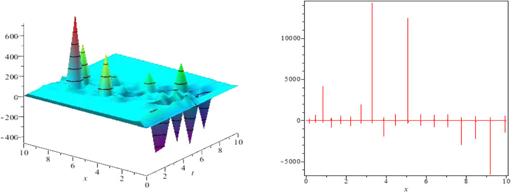
FIGURE 1. Periodic solution for Eq. 35 for $Y_{12}$ at $\omega =\frac{1}{2},k=2,a_0=1,a_1=-\frac{1}{2},\gamma \left(x,t\right)=\frac{2\cos \left(xt\right)+\left(xt\right)}{56},\delta \left(x,t\right)=\frac{2-\sin \left(xt\right)}{50},\alpha =4,\beta =5,\sigma =-3,x=4.5$.

FIGURE 2

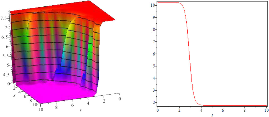
FIGURE 2. Kink-shaped solution for Eq. 35 for $Y_5$ at $\omega =2,k=3,a_0=5,a_1=5,\gamma \left(x,t\right)=\frac{2\cos \left(xt\right)+\left(xt\right)}{56},\delta \left(x,t\right)=\frac{2-\sin \left(xt\right)}{50},\alpha =4,\beta =5,\sigma =-30,x=4$.

FIGURE 3

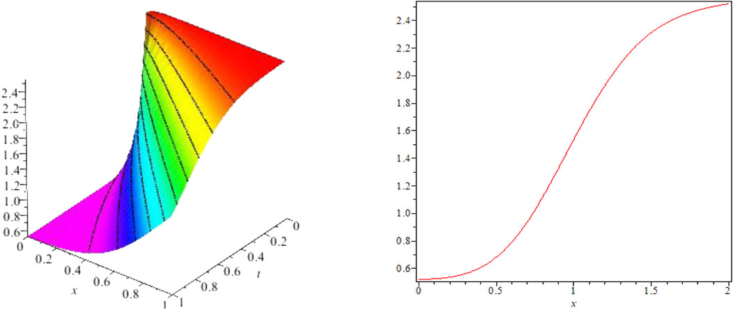
FIGURE 3. Kink-shaped solution for Eq. 35 for $Y_7$ at $\omega =1,k=1,a_0=1,a_1=-\frac{1}{2},\gamma \left(x,t\right)=\frac{20-{\left(xt\right)}^4}{50},\delta \left(x,t\right)=\frac{15+{\mathit{sin}}^6\left(xt\right)}{50},\alpha =4,\beta =5,\sigma =-3,t=1.$

FIGURE 4

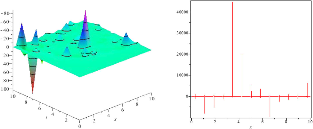
FIGURE 4. Kink-shaped solution for Eq. 35 for $Y_{23}$ at $\omega =1,k=1,a_0=1,a_1=-\frac{1}{2},\gamma \left(x,t\right)=\frac{2\mathit{cos}\left(xt\right)+\left(xt\right)}{56},\delta \left(x,t\right)=\frac{2-\mathit{sin}\left(xt\right)}{50},\alpha =4,\beta =5,\sigma =-3,e=2.7128,x=3.5$.

FIGURE 5

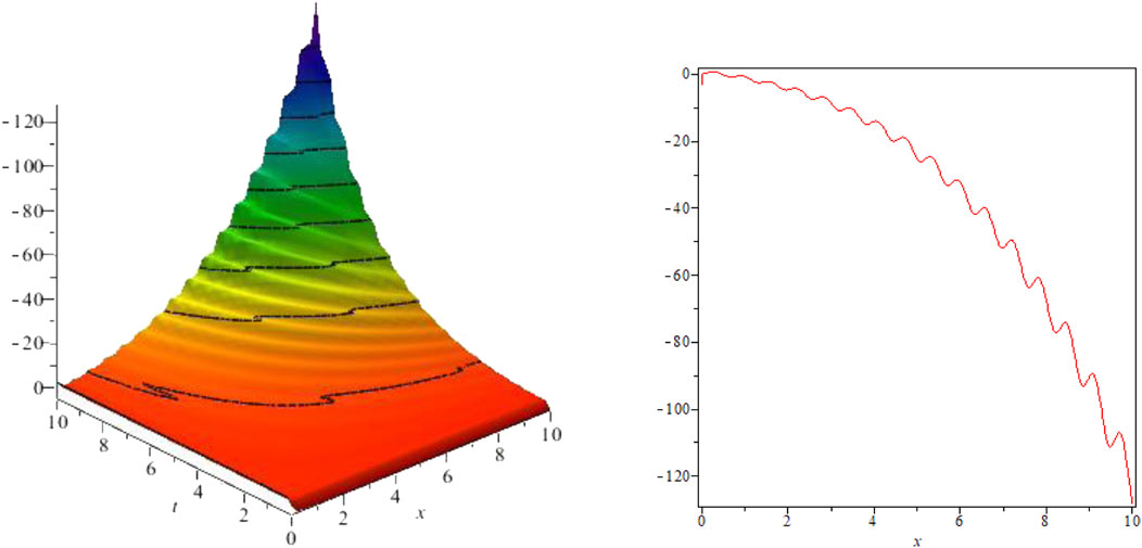
FIGURE 5. Kink-shaped solution for Eq. 35 for $Y_{24}$ at $\omega =1,k=1,a_0=1,a_1=-\frac{1}{2},\gamma \left(x,t\right)=\frac{2\cos \left(xt\right)+\left(xt\right)}{56},\delta \left(x,t\right)=\frac{2-\mathit{sin}\left(xt\right)}{50},\alpha =4,\beta =5,\sigma =-3,e=2.7128,z=1$.

5 Conclusion

In this paper, we solved the non-linear VO fractional evolution equation successfully in the Caputo fractional derivative sense and obtained new exact traveling wave solutions. The VO fractional evolution equation is discussed quite efficiently and accurately by using the Khater method. Here, 27 exact solutions having Kink and singular soliton-type solutions are obtained for different values of VO $\gamma \left(x,t\right)$ and $\delta \left(x,t\right)$ for the proposed Caputo fractional VO equation. The different values of parameters examine different physical phenomena. This contribution is effective, instrumental, and evangelistic and seems more natural in the literature. This study can be extended to other types of VO FPDEs and can be solved by various analytical techniques.

Data availability statement

The raw data supporting the conclusion of this article will be made available by the authors, without undue reservation.

Author contributions

All authors listed have made a substantial, direct, and intellectual contribution to the work and approved it for publication.

Funding

The authors would like to thank the Deanship of Scientific Research at Umm Al-Qura University for supporting this work under grant code: 22UQU4310396DSR54.

Conflict of interest

The authors declare that the research was conducted in the absence of any commercial or financial relationships that could be construed as a potential conflict of interest.

Publisher’s note

All claims expressed in this article are solely those of the authors and do not necessarily represent those of their affiliated organizations, or those of the publisher, the editors, and the reviewers. Any product that may be evaluated in this article, or claim that may be made by its manufacturer, is not guaranteed or endorsed by the publisher.

Abbreviations

ADI, alternating direction implicit scheme; EW, equal width; FPDE, fractional partial differential equation; GEW, generalized equal width; ODE, ordinary differential equation; SRLW, symmetric regularized long wave; VO, variable order; 2D, two-dimensional; 3D, three-dimensional.

References

1. Bekir A, Güner Ö. The G′G-expansion method using modified Riemann–Liouville derivative for some space-time fractional differential equations. Ain Shams Eng J (2014) 5(3):959–65. doi:10.1016/j.asej.2014.03.006

CrossRef Full Text | Google Scholar

2. Bin Z. (G′/G)-expansion method for solving fractional partial differential equations in the theory of mathematical physics. Communic Theor Phys (2012) 58:623–30. doi:10.1088/0253-6102/58/5/02

CrossRef Full Text | Google Scholar

3. Akgül A, Baleanu D. On solutions of variable-order fractional differential equations. Int J Optimization Control Theories Appl (Ijocta) (2017) 7(1):112–6. doi:10.11121/ijocta.01.2017.00368

CrossRef Full Text | Google Scholar

4. Katsikadelis JT. Numerical solution of variable order fractional differential equations (2018). Available at: https://arXiv.org/abs/preprint.arXiv:1802.00519.

Google Scholar

5. Sahoo S, Saha Ray S, Das S, Bera RK. The formation of dynamic variable order fractional differential equation. Int J Mod Phys C (2016) 27(07):1650074. doi:10.1142/s0129183116500741

CrossRef Full Text | Google Scholar

6. Singh AK, Mehra M, Gulyani S. Learning parameters of a system of variable order fractional differential equations. Numer Methods Partial Differential Equations (2021) num.22796. doi:10.1002/num.22796

CrossRef Full Text | Google Scholar

7. Semary MS, Hassan HN, Radwan AG. The minimax approach for a class of variable order fractional differential equation. Math Methods Appl Sci (2019) 42(8):2734–45. doi:10.1002/mma.5545

CrossRef Full Text | Google Scholar

8. Taghipour M, Aminikhah H. A new compact alternating direction implicit method for solving two-dimensional time fractional diffusion equation with Caputo-Fabrizio derivative. Filomat (2020) 34(11):3609–26. doi:10.2298/fil2011609t

CrossRef Full Text | Google Scholar

9. Ali U, Sohail M, Usman M, Abdullah FA, Khan I, Nisar KS. Fourth-order difference approximation for time-fractional modified sub-diffusion equation. Symmetry (2020) 12(5):691. doi:10.3390/sym12050691

CrossRef Full Text | Google Scholar

10. Ali U, Kamal R, Mohyud-Din ST. On nonlinear fractional differential equations. Int J Mod Math Sci (2012) 3:3., no.

Google Scholar

11. Zhao Z, Yue J, He L. New type of multiple lump and rogue wave solutions of the (2+ 1)-dimensional Bogoyavlenskii–Kadomtsev–Petviashvili equation. Appl Math Lett (2022) 133:108294. doi:10.1016/j.aml.2022.108294

CrossRef Full Text | Google Scholar

12. Zubair T, Usman M, Ali U, Mohyud-Din ST. Homotopy analysis method fa or system of partial differential equations. Int J Mod Eng Sci (2012) 1(2):67–79.

Google Scholar

13. Zhao Z, He L. A new type of multiple-lump and interaction solution of the Kadomtsev–Petviashvili I equation. Nonlinear Dyn (2022) 109:1033–46. doi:10.1007/s11071-022-07484-6

CrossRef Full Text | Google Scholar

14. Hu W, Deng Z, Han S, Zhang W. Generalized multi-symplectic integrators for a class of Hamiltonian nonlinear wave PDEs. J Comput Phys (2013) 235:394–406. doi:10.1016/j.jcp.2012.10.032

CrossRef Full Text | Google Scholar

15. Hu W, Xu M, Song J, Gao Q, Deng Z. Coupling dynamic behaviors of flexible stretching hub-beam system. Mech Syst Signal Process (2021) 151:107389. doi:10.1016/j.ymssp.2020.107389

CrossRef Full Text | Google Scholar

16. Zhao Z, He L. Lie symmetry, nonlocal symmetry analysis, and interaction of solutions of a (2+ 1)-dimensional KdV–mKdV equation. Theor Math Phys (2021) 206(2):142–62. doi:10.1134/s0040577921020033

CrossRef Full Text | Google Scholar

17. Uddin MH, Khatun MA, Arefin MA, Akbar MA. Abundant new exact solutions to the fractional nonlinear evolution equation via Riemann-Liouville derivative. Alexandria Eng J (2021) 60(6):5183–91. doi:10.1016/j.aej.2021.04.060

CrossRef Full Text | Google Scholar

18. Barman HK, Seadawy AR, Roy R, Akbar MA, Raddadi MH. Rational closed form soliton solutions to certain nonlinear evolution equations ascend in mathematical physics. Results Phys (2021) 27:104450. doi:10.1016/j.rinp.2021.104450

CrossRef Full Text | Google Scholar

19. Barman HK, Akbar MA, Osman MS, Nisar KS, Zakarya M, Abdel-Aty AH, et al. Solutions to the Konopelchenko-Dubrovsky equation and the Landau-Ginzburg-Higgs equation via the generalized Kudryashov technique. Results Phys (2021) 24:104092. doi:10.1016/j.rinp.2021.104092

CrossRef Full Text | Google Scholar

20. Roy R, Akbar MA, Seadawy AR, Baleanu D. Search for adequate closed form wave solutions to space–time fractional nonlinear equations. Partial Differential Equations Appl Math (2021) 3:100025. doi:10.1016/j.padiff.2021.100025

CrossRef Full Text | Google Scholar

21. Kumar S, Niwas M, Osman MS, Abdou MA. Abundant different types of exact soliton solution to the (4+1)-dimensional Fokas and (2+1)-dimensional breaking soliton equations. Commun Theor Phys (2021) 73:105007. doi:10.1088/1572-9494/ac11ee

CrossRef Full Text | Google Scholar

22. Ali U, Mastoi S, Othman WAM, Khater MM, Sohail M. Computation of traveling wave solution for nonlinear variable-order fractional model of modified equal width equation. AIMS Math (2021) 6(9):10055–69. doi:10.3934/math.2021584

CrossRef Full Text | Google Scholar

23. Akhtar J, Seadawy AR, Tariq KU, Baleanu D. On some novel exact solutions to the time fractional (2+ 1) dimensional Konopelchenko–Dubrovsky system arising in physical science. Open Phys (2020) 18(1):806–19. doi:10.1515/phys-2020-0188

CrossRef Full Text | Google Scholar

24. Islam T, Akbar MA, Azad AK. Traveling wave solutions to some nonlinear fractional partial differential equations through the rational (G′/G)-expansion method. J Ocean Eng Sci (2018) 3(1):76–81. doi:10.1016/j.joes.2017.12.003

CrossRef Full Text | Google Scholar

25. Mamun Miah M, Shahadat Ali HM, Ali Akbar M, Majid Wazwaz A. Some applications of the (G′/G, 1/G)-expansion method to find new exact solutions of NLEEs. The Eur Phys J Plus (2017) 132(6):252–15. doi:10.1140/epjp/i2017-11571-0

CrossRef Full Text | Google Scholar

26. Islam MS, Khan K, Akbar MA, Mastroberardino A. A note on improved F-expansion method combined with Riccati equation applied to nonlinear evolution equations. R Soc Open Sci (2014) 1(2):140038. doi:10.1098/rsos.140038

PubMed Abstract | CrossRef Full Text | Google Scholar

27. Hu W, Huai Y, Xu M, Feng X, Jiang R, Zheng Y, et al. Mechanoelectrical flexible hub-beam model of ionic-type solvent-free nanofluids. Mech Syst Signal Process (2021) 159:107833. doi:10.1016/j.ymssp.2021.107833

CrossRef Full Text | Google Scholar

28. Hu W, Xu M, Zhang F, Xiao C, Deng Z. Dynamic analysis on flexible hub-beam with step-variable cross-section. Mech Syst Signal Process (2022) 180:109423. doi:10.1016/j.ymssp.2022.109423

CrossRef Full Text | Google Scholar

29. Ali U, Ahmad H, Abu-Zinadah H. Soliton solutions for nonlinear variable-order fractional Korteweg–de Vries (KdV) equation arising in shallow water waves. J Ocean Eng Sci (2022). doi:10.1016/j.joes.2022.06.011

CrossRef Full Text | Google Scholar

30. Gulalai SA, Rihan FA, Ullah A, Al-Mdallal QM, Akgul A. Nonlinear analysis of a nonlinear modified KdV equation under Atangana Baleanu Caputo derivative. AIMS Math (2022) 7(5):7847–65. doi:10.3934/math.2022439

CrossRef Full Text | Google Scholar

31. Hu W, Wang Z, Zhao Y, Deng Z. Symmetry breaking of infinite-dimensional dynamic system. Appl Math Lett (2020) 103:106207. doi:10.1016/j.aml.2019.106207

CrossRef Full Text | Google Scholar

32. Zayed Elsayed ME, Amer Yasser A, Shohib Reham MA. Exact traveling wave solution for nonlinear fractional partial differential equation using the improved (G’/G)-expansion method. Int J Engin (2014) 4(7):18–31.

Google Scholar

33. Ali U, Ganie AH, Khan I, Alotaibi F, Kamran K, Muhammad S, et al. Traveling wave solutions to a mathematical model of fractional order (2+ 1)-dimensional breaking soliton equation. Fractals (2022). p. 2240124.

Google Scholar

34. Hu W, Zhang C, Deng Z. Vibration and elastic wave propagation in spatial flexible damping panel attached to four special springs. Commun Nonlinear Sci Numer Simulation (2020) 84:105199. doi:10.1016/j.cnsns.2020.105199

CrossRef Full Text | Google Scholar

35. Ali U, Ahmad H, Baili J, Botmart T, Aldahlan MA. Exact analytical wave solutions for space-time variable-order fractional modified equal width equation. Results Phys (2022) 33:105216. doi:10.1016/j.rinp.2022.105216

CrossRef Full Text | Google Scholar

36. Hu W, Huai Y, Xu M, Deng Z. Coupling dynamic characteristics of simplified model for tethered satellite system. Acta Mechanica Sinica (2021) 37(8):1245–54. doi:10.1007/s10409-021-01108-9

CrossRef Full Text | Google Scholar

37. Nayfeh AH, Balachandran B. Applied nonlinear dynamics: Analytical, computational, and experimental methods. John Wiley & Sons (2008).

Google Scholar

38. Pushkarev AN, Zakharov VEE. Nonlinear amplification of ocean waves in straits. Theor Math Phys (2020) 203(1):535–546.

CrossRef Full Text | Google Scholar

39. Rezazadeh H, Korkmaz A, Khater MM, Eslami M, Lu D, Attia RA. New exact traveling wave solutions of biological population model via the extended rational sinh-cosh method and the modified Khater method. Mod Phys Lett B (2019) 33(28):1950338. doi:10.1142/s021798491950338x

CrossRef Full Text | Google Scholar

40. Clarkson PA, Mansfield EL. On a shallow water wave equation. Nonlinearity (1994) 7(3):975–1000. doi:10.1088/0951-7715/7/3/012

CrossRef Full Text | Google Scholar

41. Bagchi B, Das S, Ganguly A. New exact solutions of a generalized shallow water wave equation. Physica Scripta (2010) 82(2):025003. doi:10.1088/0031-8949/82/02/025003

CrossRef Full Text | Google Scholar