A review on analytical studies in gravitational lensing

In this study, we review some current studies on gravitational lensing for black holes, mainly in the context of general relativity. We mainly focus on the analytical studies related to lensing with references to observational results. We start with reviewing lensing in spherically symmetric Schwarzschild spacetime, showing how to calculate deflection angles before moving to the rotating counterpart, the Kerr metric. Furthermore, we extend our studies for a particular class of newly proposed solutions called black-bounce spacetimes and discuss throughout the review how to explore lensing in these spacetimes and how the various parameters can be constrained using available astrophysical and cosmological data.

1 Introduction

The importance of gravitational lensing began with Eddington’s observation of the light deflection of the Sun [1]. The experiment proved to be one of the major milestones in favor of Einstein’s theory of general relativity [2]. The theory has proved itself to be the most successful theory of classical gravity. However, GR has some hiccups in the form of singularities, not being able to understand the quantum theory of it, along with the ubiquitous nature of dark matter and dark energy, forcing us to conclude that maybe there is more to the story. Following this line of thought, efforts have been made to introduce modifications to the Einstein–Hilbert Lagrangian [3–14]. However, taking in a cue from Eddington, gravitational lensing still remains one of the most indispensable tools to check and put constraints on our theory parameters.

The theory behind gravitational lensing started when O. Lodge asked a simple question in [15] on the behavior of light in a gravitational field. Interestingly, he concluded that, unlike a convex lens, the gravitational field does not focus light rays into a focal point. However, a logarithmically shaped concave lens can indeed mimic the effect of a spherically symmetric gravitational field onto the light. Inspired by such insights, O. Chwolson came up with the possibility of observing ring-like images in cases of axial symmetry. Nowadays, these ring-like images are called Einstein rings [16, 17]. Remarkably, such images were indeed observed by J. Hewitt et al. using the Very Large Array, a collection of radio telescopes in the United States. The radio source was MG1131 + 0456, and it was found when a background (radio) Galaxy is distorted into an almost closed ring [18–20]. Later, such rings were also found in the infrared and even in the optical spectrum [21] and more recently by the James Webb Telescope [22]. Typically, the diameter ranges between a few arcseconds or less.

The discovery of quasars and such rings lead to a rapid change in the field of gravitational lensing. We are now well aware of lensing techniques such as weak lensing, where the small deformations of many background galaxies are statistically evaluated for determining the (dark) matter in a foreground Galaxy cluster, and microlensing, where the light curve of a star is registered that moves transversely to the line of sight behind a (dark and compact) mass. For a thorough exposition of gravitational lensing, including an overview of all pre-1992 observations, the reader may consult the monograph [23]. More up-to-date information can be found in [24].

In all the lensing observations mentioned previously, the bending angles are so small that a weak-field approximation for the gravitational field is applicable. A much simpler quasi-Newtonian formalism has been used. This approximation centers around a so-called lens map or lens equation, which is very intuitive. This lens map of the weak-field formalism has proven extremely useful for evaluating the aforementioned lensing phenomena. It is discussed in detail, for example, in [23]. Additional material can be found, for example, in the Living Review by Wambsganss [25], which is completely based on this approximation formalism. However, there are astrophysical scenarios where the bending angles are not small. In such cases, the weak lensing theory is not valid anymore. The objective of this review is to give an overview of the various analytical techniques used to study strong lensing and to give some insights into the relation of lensing parameters to the gravity theory itself.

This expectation is nurtured mainly by the increasing evidence of a black hole at the center of our Galaxy. Black holes arise as solutions of GR and play an important role in testing various aspects of it. Recent observations coming from the “Event Horizon Telescope” (EHT) [26–38] collaboration and LIGO, Virgo, and KAGRA collaboration [39–44] have provided us with enough observational evidence that ensures the existence of supermassive black holes. Furthermore, these observations provide a unique opportunity to test various aspects of strong gravity [45–55]. This necessitates us to go beyond weak-field approximation and consider lensing by the strong gravitational field, thereby motivating us to consider the strong-field limit of the bending angle. It provides important information about the intrinsic parameters such as spin, mass, and charge of the black holes and the parameters of the underlying gravity theory. Hence, its observational implications have been investigated in recent times¹. An analytical description of the deflection angle for the spherically symmetric black hole in the strong gravitational field has been proposed in [76]. This was further based on [77, 78]. Later, it was extended for rotating black holes in [79]. A lens equation has been derived in [77], which has been further generalized in [80] where the underlying black hole serves as a lens. Numerous investigation of Einstein rings [81] and strong gravitational lensing based on the work has been made for various black hole spacetimes and compact objects².

It should be noted that in this review, we will be focusing on the analytical computation of the deflection angle of light rays using null geodesic equations. However, there are other methods of calculating the deflection angle analytically, for instance, the material medium approach. In this approach, one maps the problem effectively to a problem of light propagation through a medium with a particular refractive index determined by the strength of the gravitational field of the original spacetime for which one wants to calculate the deflection angle. For more details, interested readers are referred to [121–133] and citations of these references.

Furthermore, in recent times, several static metrics known as the black-bounce metric have been proposed in [134–137]. What makes this spacetime interesting is that they have an extra parameter which regularizes the central singularity, unlike the usual black hole spacetime. The black-bounce spacetime interpolates between a black hole and (traversable) wormhole metric depending on the choice of underlying regularization parameters. When the solution does not admit any horizon, it corresponds to a wormhole solution. Recently, the gravitational lensing in the strong deflection limit for these black-bounce spacetimes has been studied [120, 138–141]. From the lensing perspective, this kind of spacetime provides us with extra tunable parameters; hence, it is interesting to investigate the effect of this extra parameter from the theoretical and observational points of view. In this review, besides discussing some analytical results about the computation of the strong deflection angle in the background of Schwarzschild and Kerr–Newman black holes, we also discuss the effect of this black-bounce regularization parameter on the computation of the deflection angle and, finally, on the radius of the Einstein ring.

This article is organized as follows. In Section 2, we first review the deflection angle, the angular radius of Einstein rings, and Shapiro time delay for a Schwarzschild spacetime. In Section 3, we review a general formalism of computation of the equatorial deflection angle for Kerr–Newman spacetime. Then, in Section 4, we discuss the computation of the deflection angle for the black-bounce metric. We also review the computation of the Einstein ring radius of this case and comment on its dependence on charge and regularization parameters and its observational implications. Finally, we give concluding remarks in Section 5. Some necessary details are given in Appendix A. Also, we have set the value of the speed of light c and Newton’s gravitational constant G to unity.

2 Lensing for the spherically symmetric Schwarzschild black hole

In this section, we start by reviewing gravitational lensing in the simplest setup, that is, for the Schwarzschild solution. The metric reads

$d{s}^2=-\left(1-\frac{2M}{r}\right)d{t}^2+\frac{d{r}^2}{1-\frac{2M}{r}}+r^2\left(d{\theta }^2+{\sin }^2\theta d{\varphi }^2\right).$(2.1)

The Lagrangian for the particle $\bar{L}=\frac{1}{2}{g}_{\mu \nu }(x){\dot{x}}^{\mu }{\dot{x}}^{\nu }$ reads

$\bar{L}=\frac{1}{2}{g}_{\mu \nu }\left(x\right){\dot{x}}^{\mu }{\dot{x}}^{\nu }=\frac{1}{2}\left[-\left(1-\frac{2M}{r}\right){\dot{t}}^2+\frac{{\dot{r}}^2}{1-\frac{2M}{r}}+r^2{\dot{\varphi }}^2\right].$(2.2)

We are only considering geodesics on the equatorial plane, where $\theta =\frac{\pi }{2}$. Hence, sin θ = 1 along these geodesics and since θ is fixed, every $\dot{\theta }$ component is 0. Owing to the symmetry of the solution, we have two constants of motion which we can read off from the Euler–Lagrange equations. The t-component of the equation of motion gives

$\left(1-\frac{2M}{r}\right)\dot{t}=E=\mathrm{c}\mathrm{o}\mathrm{n}\mathrm{s}\mathrm{t}\mathrm{a}\mathrm{n}\mathrm{t},$(2.3)

while the ϕ component gives

$r^2\dot{\varphi }=L=\mathrm{c}\mathrm{o}\mathrm{n}\mathrm{s}\mathrm{t}\mathrm{a}\mathrm{n}\mathrm{t}.$(2.4)

In this article, we will mainly focus on the lensing of light rays³. Hence, we will be considering the light-like trajectories with the null ray condition defined as follows:

$g_{\mu \nu }{\dot{x}}^{\mu }{\dot{x}}^{\nu }=0.$(2.5)

Hence,

$-\left(1-\frac{2M}{r}\right){\dot{t}}^2+\frac{{\dot{r}}^2}{1-\frac{2M}{r}}+r^2{\dot{\varphi }}^2=0.$(2.6)

Then, we write the r component of the equation of motion in terms of the ϕ component. To obtain that, we divide (2.3) by (2.4) and also define the impact parameter as

$\lambda =\frac{L}{E}.$(2.7)

Then, we obtain

$\frac{dt}{d\varphi }=\frac{\dot{t}}{\dot{\varphi }}=\frac{r^2}{\lambda \left(1-\frac{2M}{r}\right)}.$(2.8)

Then, using (2.6), we obtain

${\left(\frac{dr}{d\varphi }\right)}^2=\frac{r^4}{{\lambda }^2}-r^2\left(1-\frac{2M}{r}\right).$(2.9)

Eqs 2.8, 2.9 provide all the necessary information regarding the behavior of light-like geodesics. Considering Eq. 2.9 and taking the ϕ derivative of this equation, we obtain

$2\frac{dr}{d\varphi }\frac{d^{2}r}{d{\varphi }^2}=\left(\frac{4r^3}{{\lambda }^2}-2r+2M\right)\frac{dr}{d\varphi }.$(2.10)

For circular light-like geodesics, we must have $\frac{dr}{d\varphi }=0$ and $\frac{d^{2}r}{d{\varphi }^2}=0$ which gives

$\begin{array}{cc}\hfill \frac{r^4}{{\lambda }^2}-r^2\left(1-\frac{2M}{r}\right)& =0,\hfill \\ \hfill \frac{4r^3}{{\lambda }^2}-2r+2M& =0.\hfill \end{array}$(2.11)

By eliminating b from the aforementioned equations, we obtain r = 3 M. We have, thus, shown that there is a circular light-like geodesic (or photon ring) r = 3 M. As we can choose any plane through the origin as our equatorial plane, there is actually a photon ring at this radius in the sense that every great circle on this sphere is a light-like geodesic. However, the photon rings at r = 3 M are unstable in the following sense: a light-like geodesic with an initial condition that deviates slightly from that of a photon ring at r = 3 M will spiral away from r = 3 M and either go to infinity or to the horizon.

Now that we have understood how the null geodesics behave in this geometry, it is time to focus on deriving actual observable quantities that one can measure. For this, we go on to study them in the upcoming sections one by one starting with calculating deflection angles.

2.1 Formula for the deflection angle

First, we set up the problem that we want to address. We consider a light ray that comes in from infinity and then goes through a minimum radius value at r = r_min and then escapes back to infinity. Due to the geometry of spacetime around the central black hole, which for us is a Schwarzchild one, there will be a deflection. This deflection is simply because the rectilinear propagation of light will not be observed in this non-trivial geometry. The deflection angle measures the degree of this deviation from rectilinear propagation. In the following discussion, we will express this in terms of r_min and the mass of the central object.

We start out with (2.7) and determine the ratio $\frac{1}{{\lambda }^2}$ at r = r_min. This gives

$\frac{1}{{\lambda }^2}=\frac{1}{r_{\mathit{min}}^2}-\frac{2M}{r_{\mathit{min}}^3}.$(2.12)

Hence, replacing this in (2.7), we obtain

$d\varphi =\frac{\pm dr}{\sqrt{\left(\frac{1}{r_{\mathit{min}}^2}-\frac{2M}{r_{\mathit{min}}^3}\right)r^4-r^2+2Mr}},$(2.13)

which, on integrating over the coordinates of the light ray, leads to

$\begin{array}{cc}\hfill \pi +\widehat{\alpha }& =2{\int }_{r_{\mathit{min}}}^{\infty }\frac{r_{\mathit{min}}dr}{\sqrt{\left(1-\frac{2M}{r_{\mathit{min}}}\right)r^4-r_{\mathit{min}}^2{r}^2+2M{r}_{\mathit{min}}^{2}r}}\hfill \\ \hfill & =2{\int }_{r_{\mathit{min}}}^{\infty }\frac{r_{\mathit{min}}dr}{\sqrt{r^2\left(r^2-r_{\mathit{min}}^2\right)-\frac{2M}{r_{\mathit{min}}}\left(r^3-r_{\mathit{min}}^3\right)}}\hfill \\ \hfill & =2{\int }_{r_{\mathit{min}}}^{\infty }\frac{r_{\mathit{min}}dr}{\sqrt{1-\frac{2M}{r_{\mathit{min}}}\frac{\left(r^3-r_{\mathit{min}}^3\right)}{r\left(r^2-r_{\mathit{min}}^2\right)}}r\sqrt{r^2-r_{\mathit{min}}^2}}\hfill \\ \hfill & =2{\int }_{r_{\mathit{min}}}^{\infty }\left\{1+\frac{1}{2}\frac{2M}{r_{\mathit{min}}}\frac{\left(r^3-r_{\mathit{min}}^3\right)}{r\left(r^2-r_{\mathit{min}}^2\right)}+\mathcal{O}{\left(\frac{2M}{r_{\mathit{min}}}\right)}^2\right\}\frac{r_{\mathit{min}}dr}{r\sqrt{r^2-r_{\mathit{min}}^2}}\hfill \\ \hfill & =2{\int }_{r_{\mathit{min}}}^{\infty }\frac{r_{\mathit{min}}dr}{r\sqrt{r^2-r_{\mathit{min}}^2}}+\frac{2M}{r_{\mathit{min}}}{\int }_{r_{\mathit{min}}}^{\infty }\frac{\left(r^3-r_{\mathit{min}}^3\right)r_{\mathit{min}}dr}{r^2{\left(r^2-r_{\mathit{min}}^2\right)}^{3/2}}+\mathcal{O}{\left(\frac{2M}{r_{\mathit{min}}}\right)}^2\hfill \\ \hfill & =\pi +\frac{4M}{r_{\mathit{min}}}+\mathcal{O}{\left(\frac{2M}{r_{\mathit{min}}}\right)}^2.\hfill \end{array}$(2.14)

By neglecting higher-order terms, we obtain

$\widehat{\alpha }=\frac{4M}{r_{\mathit{min}}}.$(2.15)

Now, we will look at a point or two about this derivation:

• From the derivation, it is clear that the integrand has a singularity at the lower bound r = r_min. A more detailed analysis shows that the integral is finite for all values of r = r_min that are bigger than $\frac{3}{2}{r}_s$, where r_s = 2 M. If we consider a sequence of light rays with r = r_min approaching $\frac{3}{2}{r}_s$ from earlier, the deflection angle δ becomes bigger and bigger, which means that the light rays make more and more turns around the center. In the limit $r_{\mathit{min}}\to \frac{3}{2}{r}_s$, the integral goes to infinity, and the limiting light ray spirals asymptotically toward a circle at $r=\frac{3}{2}{r}_s$. If an unstable photon ring is approached, the deflection angle goes to infinity, and the singularity is logarithmic.

• The second point comes during the discussion on taking the Taylor series expansion in $\frac{r_s}{r_{\mathit{min}}}$ in the fourth step. The asymptotic behavior of light rays for r_min approaching $\frac{3}{2}{r}_s$ is relevant only for black holes and for ultracompact stars. For an ordinary star, like our Sun, r_min takes a value much bigger than r_s. It is under this consideration that we take a Taylor series expansion in $\frac{r_s}{r_{\mathit{min}}}$.

2.2 Shapiro time

Combining Eqs. 2.8 and 2.9 allows us to calculate the time taken by the light ray in this particular geometry. Here, we consider a light ray that starts at a radius r_L, passes through a minimum of radius r_min, and terminates at a radius r_o. From Eqs. 2.8 and 2.9, we obtain

$\begin{array}{ll}\hfill {\left(\frac{dr}{dt}\right)}^2& ={\left(\frac{dr}{d\varphi }\right)}^2{\left(\frac{d\varphi }{dt}\right)}^2=\left\{\frac{r^4}{{\lambda }^2}-r^2\left(1-\frac{2M}{r}\right)\right\}\frac{{\left(1-\frac{2M}{r}\right)}^2}{{\lambda }^2{r}^4}\hfill \\ \hfill & =\left\{\frac{r^3}{{\lambda }^2}-r\left(1-\frac{2M}{r}\right)\right\}\frac{{\left(r-2M\right)}^2}{{\lambda }^2{r}^5}.\hfill \end{array}$(2.16)

At r = r_min, (2.16) reads

$\frac{r_{\mathit{min}}^4}{{\lambda }^2}-r_{\mathit{min}}^2\left(1-\frac{2M}{r_{\mathit{min}}}\right)=0\Rightarrow \frac{1}{{\lambda }^2}=\frac{r_{\mathit{min}}-2M}{r_{\mathit{min}}^3}.$(2.17)

Finally, (2.16) becomes

${\left(\frac{dr}{dt}\right)}^2=\left\{\frac{\left(r_{\mathit{min}}-2M\right)r^3}{r_{\mathit{min}}^3}-r\left(1-\frac{2M}{r}\right)\right\}\frac{\left(r-2M\right)r_{\mathit{min}}^3}{\left(r_{\mathit{min}}-2M\right)r^5},$(2.18)

which gives

$dt=\frac{\pm \sqrt{r_{\mathit{min}}-2M}{r}^{5/2}dr}{\left(r-2M\right)r_{\mathit{min}}^{3/2}\sqrt{\frac{\left(r_{\mathit{min}}-2M\right)r^3}{r_{\mathit{min}}^3}-r\left(1-\frac{2M}{r}\right)}}.$(2.19)

By integrating, we obtain the travel time for the light ray,

$\mathrm{\Delta }t=\left(-{\int }_{r_L}^{r_{\mathit{min}}}+{\int }_{r_{\mathit{min}}}^{r_O}\right)\frac{\sqrt{r_{\mathit{min}}-2M}{r}^{5/2}dr}{\left(r-2M\right)r_{\mathit{min}}^{3/2}\sqrt{\frac{\left(r_{\mathit{min}}-2M\right)r^3}{r_{\mathit{min}}^3}-r\left(1-\frac{2M}{r}\right)}},$(2.20)

where the signs on the right-hand side had to be chosen in such a way that the time coordinate is always increasing along the light ray. One can perform this integral exactly in terms of an elliptic integral. However, when r_min ≫ r_s, we can make a Taylor approximation, in exactly the same way as we did it for the deflection formula, and obtain

$\begin{array}{cc}\hfill \mathrm{\Delta }t& =\left({\int }_{r_{\mathit{min}}}^{r_L}+{\int }_{r_{\mathit{min}}}^{r_O}\right)\frac{rdr}{\sqrt{r^2-r_{\mathit{min}}^2}}+2M\left({\int }_{r_{\mathit{min}}}^{r_L}+{\int }_{r_{\mathit{min}}}^{r_O}\right)\frac{dr}{\sqrt{r^2-r_{\mathit{min}}^2}}\hfill \\ \hfill & +\frac{2M{r}_{\mathit{min}}}{2}\left({\int }_{r_{\mathit{min}}}^{r_L}+{\int }_{r_{\mathit{min}}}^{r_O}\right)\frac{dr}{\sqrt{r-r_{\mathit{min}}}{\left(r+r_{\mathit{min}}\right)}^{3/2}}+\cdots \hfill \end{array}$(2.21)

The zeroth-order term is, of course, the Euclidean travel time for a light ray with speed c along a straight line. The deviation of the general-relativistic calculation from this zeroth-order term is known as the Shapiro time delay [142].

I. Shapiro suggested using this effect as the fourth test of general relativity (after perihelion precession, light deflection, and gravitational redshift). In the first experiment, a strong radio signal was sent to Venus when it was in opposition to Earth, and the time was measured until the signal arrived back on Earth after being reflected in Venus’s atmosphere. Later experiments were performed with transponders on spacecraft, which sent the signal back with increased intensity. The best measurement to date was performed with the Cassini spacecraft in 2002. The general-relativistic time delay was verified to be within an accuracy of 0.001% [142].

2.3 Angular radius of Einstein rings

An Einstein ring can be observed when the light source and observer are perfectly aligned (directly opposite to each other). We want to determine the angular radius θ_E of the Einstein ring in dependence on the radius coordinate r_L of the light source, the radius coordinate r_O of the observer, and the Schwarzschild radius (= 2M). We use the formula

$d\varphi =\frac{\pm dr}{\sqrt{\frac{\left(r_{\mathit{min}}-\frac{2M}{c^2}\right)r^4}{r_{\mathit{min}}^3}-r^2+2Mr}}.$(2.22)

Integrating over the light ray gives

$\pi =\left({\int }_{r_{\mathit{min}}}^{r_L}+{\int }_{r_{\mathit{min}}}^{r_O}\right)\frac{dr}{\sqrt{\frac{\left(r_{\mathit{min}}-\frac{2M}{c^2}\right)r^4}{r_{\mathit{min}}^3}-r^2+2Mr}}.$(2.23)

The integration gives

$r_{\mathit{min}}=f\left(r_L,r_O,2M\right).$(2.24)

With r_min determined, the angular radius of the Einstein ring can be obtained by

$\tan {\theta }_E=\frac{rd\varphi }{{\left(1-\frac{2M}{r}\right)}^{-1/2}dr}{|}_{r=r_O}.$(2.25)

3 Lensing for the Kerr–Newman black hole

In Section 2, we discussed the gravitational lensing in Schwarzschild spacetime. We expand the integrand around the turning point to obtain a simplified result, but in principle, we can calculate the exact deflection angle. In this section, first and foremost, we will generalize the result of lensing for rotating spacetime. We will calculate the deflection angle for the light rays in Kerr–Newman spacetime which is an axisymmetric spacetime. One can reproduce the result for the Kerr and Schwarzschild case as special limits. We will also discuss the strong deflection angle’s analytical form. We will closely follow the notation in [120].

In Boyer–Lindquist, the line element is given by

$d{s}^2=-\frac{\mathrm{\Delta }}{\mathrm{\Sigma }}{\left(dt-a{\sin }^2\theta d\varphi \right)}^2+\mathrm{\Sigma }\left(\frac{d{r}^2}{\mathrm{\Delta }}+d{\theta }^2\right)+\frac{{\sin }^2\theta }{\mathrm{\Sigma }}{\left(adt-\left(r^2+a^2\right)d\varphi \right)}^2,$(3.1)

where

$\mathrm{\Sigma }=r^2+a^2{\cos }^2\theta ,\mathrm{\Delta }\left(r\right)=\mathrm{\Delta }\left(r\right)=\left(r^2+a^2\right)-2mr+Q^2.$(3.2)

In (3.3) and (3.2), m ≥ 0, Q, and a are, respectively, the ADM mass, charge, and angular momentum of the black hole. As we know, the particle Lagrangian, specifically for the photons, is given by (2.2), with ${\dot{x}}^{\mu }=\frac{d{x}^{\mu }}{d\tilde{\lambda }}$ for some convenient parameter $\tilde{\lambda }$. The metric coefficients are independent of t and ϕ, implying that we will have two conserved quantities along the photon trajectory: energy E and angular momentum L. Using the constants of motion and the null ray condition in (2.5), the null geodesic equations can be written as follows:

$\begin{array}{cc}\hfill {\rho }^4{\dot{r}}^2& ={\left(\left(r^2+a^2\right)E-aL\right)}^2-\mathrm{\Delta }\left(r\right)\left({\left(L-aE\right)}^2+\bar{K}\right)≔R^2\left(r\right),\hfill \\ \hfill \mathrm{\Sigma }\dot{\varphi }& =-\left(aE-\frac{L}{{\sin }^2\theta }\right)+\frac{a\left[E\left(r^2+a^2\right)-aL\right]}{\mathrm{\Delta }},\hfill \\ \hfill \mathrm{\Sigma }\dot{t}& =-a\left(aE{\sin }^2\theta -L\right)+\frac{\left(r^2+a^2\right)\left[E\left(r^2+a^2\right)-aL\right]}{\mathrm{\Delta }},\hfill \\ \hfill {\rho }^4{\dot{\theta }}^2& =\bar{K}+{\cos }^2\theta \left(a^2{E}^2-\frac{L^2}{{\sin }^2\theta }\right)≔\mathrm{\Theta }{\left(\theta \right)}^2\hfill \end{array}$(3.3)

where the Carter constant, which results from the separability of the Hamilton–Jacobi equation, is $\bar{K}$. For our purpose, we will look upon into the equatorial case only, that is, $\theta =\frac{\pi }{2},\dot{\theta }=0$ which automatically implies $\bar{K}=0$, and then will investigate the non-equatorial case also. We can use the geodesic equations to calculate the equatorial deflection angle. Rather in the next section, we will provide the deflection angle calculations and reproduce the result for Kerr by taking the limit Q = 0.

3.1 Deflection angle for Kerr–Newman spacetime

From (3.3), we can write the radial geodesic equations as follows:

$\frac{{\dot{r}}^2}{L^2}+V\left(r\right)=\frac{1}{{\lambda }^2},$(3.4)

with the effective potential

$V\left(r\right)=\frac{1}{r^2}\left[1-\frac{a^2}{{\lambda }^2}+{\left(1-\frac{a}{\lambda }\right)}^2\left(-\frac{2m}{r}+\frac{Q^2}{r^2}\right)\right],$(3.5)

and λ is the impact parameter defined in (2.7).

Now, we think of light rays that originate at infinity, pass through the black hole, and then, return to infinity to reach the observer. The closest approach to the black hole, r₀, will be the radial turning point for these light rays, determined by

${\left.\left(\frac{{\dot{r}}^2}{L^2}\right)\right|}_{r=r_0}=\frac{1}{{\lambda }^2}-V\left(r_0\right)=0.$(3.6)

From (3.6), we obtain

${r_0}^4-{\lambda }^2\left(1-\frac{a^2}{{\lambda }^2}\right){r_0}^2+2m{\lambda }^2{\left(1-\frac{a}{\lambda }\right)}^2{r}_0=Q^2{\lambda }^2{\left(1-\frac{a}{\lambda }\right)}^2.$(3.7)

Solving (3.7), we obtain

$\begin{array}{c}\hfill r_0\left(\lambda \right)=\frac{\lambda }{\sqrt{6}}\sqrt{1-{\omega }^2}\left[\sqrt{1+\widehat{\gamma }}+\sqrt{2-\widehat{\gamma }-\frac{3\sqrt{6}m{\left(1-\omega \right)}^2}{\lambda {\left(1-{\omega }^2\right)}^{3/2}\sqrt{1+\widehat{\gamma }}}}\right]\end{array},$(3.8)

where $\omega ,\chi ,\rho ,\widehat{\gamma }$ are given by

$\begin{array}{cc}\hfill \omega & =\frac{a}{\lambda },\rho =\frac{12Q^2}{{\lambda }^2{\left(1+\omega \right)}^2},\widehat{\gamma }=\sqrt{1-\rho }\cos \left(\frac{2\chi }{3}\right),\hfill \\ \hfill \chi & =\arccos \left(\frac{3\sqrt{3}m{\left(1-\omega \right)}^2}{\lambda {\left(1-{\omega }^2\right)}^{3/2}{\left(1-\rho \right)}^{3/4}}\sqrt{1-\frac{{\lambda }^2{\left(1+\omega \right)}^3}{54m^2\left(1-\omega \right)}\left[1+3\rho -{\left(1-\rho \right)}^{3/2}\right]}\right).\hfill \end{array}$(3.9)

One can convince that the non-zero charge of the black holes gives a repulsive effect on the light rays, but the effect of spin attracts the light rays toward the black hole.

3.2 Photon sphere radius and critical impact parameter

In this subsection, we will define the photon sphere and the critical impact parameter which will be useful in the subsequent sections. The radius of the photon sphere is the value of r where the effective potential attains its maximum value.

${\left.\frac{\partial V\left(r\right)}{\partial r}\right|}_{r=r_c}=0.$(3.10)

From (3.10), we can find out

$r_c\left({\lambda }_c\right)=\frac{3m\widehat{\zeta }}{2}\left[1+\sqrt{1-\zeta }\right],$(3.11)

where

$\widehat{\zeta }=\left(\frac{1-\frac{a}{{\lambda }_c}}{1+\frac{a}{{\lambda }_c}}\right),\zeta =\frac{8Q^2}{9m^2}\widehat{\zeta }.$

It should be noted that the turning point of the photon is r₀ defined in (3.8) and attains its minimum value at r_c with the corresponding impact parameter λ_c. If for some λ, r₀ becomes less than r_c, then the photon will fall into the black hole. λ_c is called the critical impact parameter. Finally, substituting Eq. 3.8 into (3.11), we can write λ_c = λ_c(a, Q, l) and r_c = r_c(a, Q, l).

3.3 An exact analytical computation of the deflection angle

In this subsection, we will compute the exact photon deflection angle near a Kerr–Newman black hole. To perform this, we can choose any polar plane, but to keep things simple, we choose the equatorial plane $\theta =\frac{\pi }{2}$ and $\dot{\theta }=0$. Furthermore, to investigate the observational signature, we need to employ the strong deflection limit. To perform this, we have to evaluate the deflection angle in the mentioned plane and take the strong limit. We can rather perform the reverse procedure also; that is, from the beginning, we take the strong limit and then calculate the deflection angle at this limit. The second one is simpler to perform. We adopt this track while discussing the observational signature.

The analysis has been performed in [143, 144]. We review the analysis here. Before proceeding with the computation, we define the following coordinates:

$u≔\frac{1}{r}.$(3.12)

By combining the first two equations in (3.3), we obtain

${\left(\frac{du}{d\varphi }\right)}^2={\left(\frac{du}{dr}\frac{dr}{d\varphi }\right)}^2=\frac{r^2}{r^6}\frac{{\dot{r}}^2}{{\dot{\varphi }}^2}=\left(u^4\right)\frac{{\dot{r}}^2}{{\dot{\varphi }}^2}.$(3.13)

Now, our goal is to rewrite $\dot{r}$ and $\dot{\varphi }$ as a function of u. We have

$\begin{array}{ll}\hfill {\dot{r}}^2& =L^2\left(\frac{1}{{\lambda }^2}-V\left(r\right)\right)\hfill \\ \hfill & =L^2\left[\frac{1}{{\lambda }^2}-\left[\frac{1}{r^2}\left(1-\frac{a^2}{{\lambda }^2}+{\left(1-\frac{a}{\lambda }\right)}^2(-\frac{2m}{r}+\frac{Q^2}{r^2}\right)\right]\right]\hfill \\ \hfill & =L^2\left[\frac{1}{{\lambda }^2}-u^2\left(1-\frac{a^2}{{\lambda }^2}\right)-Q^2{\left(1-\frac{a}{\lambda }\right)}^2{u}^4+2m{\left(1-\frac{a}{\lambda }\right)}^2{u}^3\right]≔L^{2}B\left(u\right).\hfill \end{array}$(3.14)

Combining Eqs 3.14 and 3.3 and using Eq. 3.13, we obtain

${\left(\frac{du}{d\varphi }\right)}^2={\left[\frac{1-2mu+\left(a^2+Q^2\right)u^2}{1-\left(2mu-Q^2{u}^2\right)\left(1-\frac{a}{\lambda }\right)}\right]}^{2}B\left(u\right).$(3.15)

The photon deflection angle $\widehat{\alpha }$ can be calculated by integrating Eq. 3.15 over u from 0 to $\frac{1}{\sqrt{r}}$, where r₀ is the turning point, and then evaluating the resulting expression at the critical value r_c [79],

$\widehat{\alpha }=-\pi +2{\int }_0^{\frac{1}{r_0}}du\left[\frac{1-\left(2mu-Q^2{u}^2\right)\left(1-\frac{a}{\lambda }\right)}{1-2mu+\left(a^2+Q^2\right)u^2}\right]\frac{1}{\sqrt{B\left(u\right)}},$(3.16)

with $\omega =\frac{a}{\lambda }$. This integral can be computed exactly. We give the final result here. The details of the computation of this integral are given in Appendix A.

$\begin{array}{cc}\hfill \widehat{\alpha }& =-\pi +\frac{4}{\left(1-\omega \right)\sqrt{Q^2\left(u_4-u_2\right)\left(u_3-u_1\right)}}\hfill \\ \hfill & \times \left[\frac{G_{+}+K_{Q_{+}}{u}_1}{u_{+}-u_1}\left[\mathrm{\Pi }\left(n_{+},k\right)-\mathrm{\Pi }\left(n_{+},\varphi ,k\right)\right]+\frac{G_{-}+K_{Q_{-}}{u}_1}{u_{-}-u_1}\left[\mathrm{\Pi }\left(n_{+},k\right)-\mathrm{\Pi }\left(n_{+},\varphi ,k\right)\right]\right.\hfill \\ \hfill & -\frac{G_{+}+K_{Q_{+}}{u}_4}{u_{+}-u_4}\left[\mathrm{\Pi }\left(n_{+},k\right)-\mathrm{\Pi }\left[n_{+},\varphi ,k\right]-F\left(\frac{\pi }{2},k\right)+F\left(\varphi ,k\right)\right]\hfill \\ \hfill & \left.-\frac{G_{-}+K_{Q_{-}}{u}_4}{u_{-}-u_4}\left[\mathrm{\Pi }\left(n_{-},k\right)-\mathrm{\Pi }\left[n_{-},\varphi ,k\right]-F\left(\frac{\pi }{2},k\right)+F\left(\varphi ,k\right)\right]\right],\hfill \end{array}$(3.17)

where

$\begin{array}{ll}\hfill u_1& =\frac{X_1-2m-X_2}{4m{r}_0},u_2=\frac{1}{r_0},u_3=\frac{X_1-2m+X_2}{4m{r}_0},u_4=\frac{2m}{Q^2}-\frac{X_1}{2m{r}_0},\hfill \\ \hfill n_{\pm }& =\frac{u_2-u_1}{u_{\pm }-u_1}\left[1+\frac{2m{Q}^2\left(1-r_0{u}_{\pm }\right)}{4m^2{r}_0-Q^2\left(X_1+2m\right)}\right],\hfill \\ \hfill k^2& =\frac{\left(X_2+6m-X_1\right)\left[8m^2{r}_0-Q^2\left(X_2-2m+3X_1\right)\right]}{4X_2\left[4m^2{r}_0-Q^2\left(X_2+2m\right)\right]},\hfill \\ \hfill {\psi }_0& =\arcsin \sqrt{\frac{\left(X_2+2m-X_1\right)\left[4m^2{r}_0-Q^2\left(X_2+2m\right)\right]}{\left(X_2+6m-X_1\right)\left(4m^2{r}_0-Q^2{X}_1\right)}},\hfill \\ \hfill G_{+}& =\frac{2m\left(1-\omega \right)\left(m+\sqrt{m^2-\left(a^2+Q^2\right)}\right)-\left(a^2+Q^2\right)}{2\left(a^2+Q^2\right)\sqrt{m^2-\left(a^2+Q^2\right)}},\hfill \\ \hfill G_{-}& =\frac{\left(a^2+Q^2\right)-2m\left(1-\omega \right)\left(m-\sqrt{m^2-\left(a^2+Q^2\right)}\right)}{2\left(a^2+Q^2\right)\sqrt{m^2-\left(a^2+Q^2\right)}},\hfill \\ \hfill G_{Q+}& =\frac{-Q^2\left(1-\omega \right)\left(m+\sqrt{m^2-\left(a^2+Q^2\right)}\right)}{2\left(a^2+Q^2\right)\sqrt{m^2-\left(a^2+Q^2\right)}},\hfill \\ \hfill G_{Q-}& =\frac{Q^2\left(1-\omega \right)\left(m-\sqrt{m^2-\left(a^2+Q^2\right)}\right)}{2\left(a^2+Q^2\right)\sqrt{m^2-\left(a^2+Q^2\right)}}.\hfill \end{array}$(3.18)

It should be noted that Π(n₊, ψ₀, k) and Π(n₊, k) are the incomplete and complete elliptic integral of the third kind, respectively. Also, F(ψ₀, k) and $F(\frac{\pi }{2},k)$ are the incomplete and complete elliptic integral of the first kind, respectively. Also,

$\begin{array}{c}\hfill X_1=\frac{2m\left(Q^2+4m{r}_0\right)}{3Q^2}+\frac{8m^2{r}_0}{3Q^2}\sqrt{1+\frac{Q^2}{2m^2}\left(\frac{m}{r_0}-\frac{3\left(1+\omega \right)}{2\left(1-\omega \right)}-\frac{Q^2}{r_0^2}\right)}\cos \left(\frac{\delta }{3}+\frac{2\pi }{3}\right),\end{array}$(3.19)

where

$\begin{array}{c}\hfill \delta =\arccos \left(\frac{-8m^3{r}_0^3-3m{Q}^2{r}_0^2\left(2m-\frac{3r_0\left(1+\omega \right)}{\left(1-\omega \right)}\right)-3Q^4{r}_0\left(5m-\frac{3r_0\left(1+\omega \right)}{\left(1-\omega \right)}\right)+10Q^6}{{\left[4m^2{r}_0^2+Q^2{r}_0\left(2m-\frac{3r_0\left(1+\omega \right)}{\left(1-\omega \right)}\right)-2Q^4\right]}^{3/2}}\right)\end{array},$(3.20)

and X₂ can be obtained from the following equations after inserting X₁ from (3.20).

$\left[X_2^2-{\left(X_1^2-2m\right)}^2\right]\left(\frac{1}{8m{r}_0^3}-\frac{Q^2{X}_1}{32m^3{r}_0^4}\right)=\frac{1}{{\lambda }^2{\left(1-\omega \right)}^2}.$(3.21)

So, the exact deflection angle can be derived as discussed. One can reproduce the results for the Schwarzschild black hole in the limit a → 0 and Q → 0 and the Kerr black hole in the limit a → 0.

3.4 Strong deflection analysis for axisymmetric spacetime

In this section, we inspect the strong limit of the equatorial deflection angle $(\theta =\frac{\pi }{2})$ of the light rays discussed in the previous section in order to gain further understanding of the deflection angle for our context and make touch with the feasible observational signature. The strong deflection limit of (4.14) is challenging to take directly. It will be simpler to perform the integration after taking the strong-field limit of the integrand of (4.4). We shall only take into account the photons having the turning point very close to the photon sphere’s radius, as was previously specified.

The metric on the equatorial plane has the following structure:

$d{s}^2=-\bar{A}\left(r\right)d{t}^2+\bar{B}\left(r\right)d{r}^2+\bar{C}\left(r\right)d{\varphi }^2-\bar{D}\left(r\right)dtd\varphi ,$(3.22)

with

$\begin{array}{cc}\hfill & \bar{A}\left(r\right)=\frac{\left(\mathrm{\Delta }\left(r\right)-a^2\right)}{\mathrm{\Sigma }},\bar{B}\left(r\right)=\frac{\mathrm{\Sigma }}{\mathrm{\Delta }},\bar{C}\left(r\right)=\frac{1}{\mathrm{\Sigma }}\left[{\left(r^2+a^2+l^2\right)}^2-\mathrm{\Delta }\left(r\right)a^2\right],\hfill \\ \hfill & \bar{D}\left(r\right)=\frac{2}{\mathrm{\Sigma }}\left[\left(r^2+a^2+l^2\right)a-\mathrm{\Delta }\left(r\right)a\right].\hfill \end{array}$(3.23)

It should be noted that all metric components are evaluated in the equatorial plane. We have already seen that the spacetime admits two conserved quantities E and L due to the existing symmetries. To keep things simple, we set E = 1. As a result, the impact parameter is λ = L. Using the fact that at the distance of closest approach, r = r₀ and $\dot{r}=0$, we obtain the following results from (3.4):

$\begin{array}{cc}\hfill L& =\frac{-{\bar{D}}_0+\sqrt{4{\bar{A}}_0{\bar{C}}_0+{\bar{D}}_0^2}}{2{\bar{A}}_0}\hfill \\ \hfill & =\frac{r_0\left(r_0^2\sqrt{a^2-2m{r}_0+Q^2+r_0^2}+a\left(Q^2-2m{r}_0\right)\right)}{Q^2{r}_0+l^2\left(r_0-2m\right)+r_0^2\left(r_0-2m\right)}.\hfill \end{array}$(3.24)

The subscript “0” denotes that functions are evaluated at r = r₀. From the equation of motion of ϕ [the second equation of (3.3)], we obtain

$\varphi \left(r_0\right)=2{\int }_{r_0}^{\infty }\frac{\sqrt{\bar{B}{\bar{A}}_0}\left(\bar{D}+2L\bar{A}\right)}{\sqrt{4\bar{A}C+{\bar{D}}^2}\sqrt{{\bar{C}A}_0-{\bar{A}C}_0+L\left({\bar{A}D}_0-{\bar{D}A}_0\right)}}dr.$(3.25)

In the strong limit, we only consider the photons having closest approach r_c near to the radius of the photon sphere. To implement the limit, one can expand the deflection angle $\widehat{\alpha }$ around r_c or λ_c and perform the radial integral function. When the turning point r₀ is greater than the radius of the photon sphere r_c, then we obtain a finite deflection angle; otherwise, the photon will be caught by the black hole and the deflection angle diverges. Following the method developed here [76, 79], it is easy to find out the nature of the divergence in the deflection angle when the photons are very close to the radius of the photon sphere r = r_c. One can define two variables y, z as

$z_1=\bar{A}\left(r\right),z_2=\frac{z_1-z_{\mathrm{1,0}}}{1-z_{\mathrm{1,0}}}.$(3.26)

Now, the azimuthal angle defined in (3.25) can be expressed in terms of these two new variables,

$\varphi \left(r_0\right)={\int }_0^1\bar{R}\left(z_2,r_0\right)\bar{F}\left(z_2,r_0\right)d{z}_2,$(3.27)

where

$\bar{R}\left(z_2,r_0\right)=\frac{2\left(1-z_{\mathrm{1,0}}\right)}{A^{\prime }}\frac{\sqrt{\bar{B}{\bar{A}}_0}\left(\bar{D}+2L\bar{A}\right)}{\sqrt{4{\bar{A}C}^2+{\bar{C}D}^2}},$(3.28)

$\bar{F}\left(z_2,r_0\right)=\frac{1}{\sqrt{\frac{1}{\bar{C}}\left({\bar{C}A}_0-{\bar{A}C}_0+L\left({\bar{A}D}_0-{\bar{D}A}_0\right)\right)}}=\frac{1}{\sqrt{\bar{H}}},$(3.29)

$\bar{H}=\frac{1}{\bar{C}}\left({\bar{C}A}_0-{\bar{A}C}_0+L\left({\bar{A}D}_0-{\bar{D}A}_0\right)\right).$(3.30)

The function $\bar{R}(z,r0)$ is regular for any z and r₀ values, whereas the function $\bar{F}(z,r0)$ is divergent for z = 0, that is, at r = r₀. As a result, after extracting the divergent part, one can rewrite (3.25).

$\varphi \left(r_0\right)={\varphi }_{\bar{R}}\left(r_0\right)+{\varphi }_{\bar{F}}\left(r_0\right),$(3.31)

where the divergent part can be written as follows:

${\varphi }_{\bar{F}}\left(r_0\right)={\int }_0^1\bar{R}\left(z_2=0,r_c\right){\bar{F}}_0\left(z_2,r_0\right)dz.$(3.32)

We know that the deflection angle should diverge at r₀ = r_c, indicating that the photon has been captured by the black hole. Next, we want to determine the nature of the divergence. Examining the denominator will allow us to determine the nature of the divergence (4.18). In order to achieve this, we Taylor expand the denominator of ${\bar{F}}_0(r_0,z_2)$ (3.33) around z₂ = 0.

${\bar{F}}_0\left(z_2,r_0\right)\approx \frac{1}{\sqrt{{\sigma }_1\left(r_0\right)z+{\sigma }_2\left(r_0\right)z_2^2+\mathcal{O}\left(z^3\right)}}.$(3.33)

It is worth noting that if σ₁(r₀) = 0 (this occurs when r₀ coincides with the radius of the photon sphere [145]), then it is clear from (3.33) that the leading term is $\frac{1}{z}$ in the small z limit. As a result, after integration, we obtain a logarithmic divergence, as shown in (3.42). To find σ₁ and σ₂, we first Taylor expand $\bar{H}$, which is defined in (4.21).

$\bar{H}\left(z,r_0\right)=\bar{H}\left(0,r_0\right)+{\left.\frac{\partial \bar{H}}{\partial z_2}\right|}_{z_2=0}{z}_2+\frac{1}{2!}{\left.\frac{{\partial }^2\bar{H}}{\partial z_2^2}\right|}_{z_2=0}{z}_2^2+\mathcal{O}\left(z_2^3\right),\text{with}\bar{H}\left(0,r_0\right)=0.$(3.34)

Therefore, using (4.20), we can identify σ₁ and σ₂ as

$\begin{array}{ll}\hfill {\sigma }_1& ≔{\left.\frac{\partial \bar{H}}{\partial z_2}\right|}_{z_2=0}\hfill \\ \hfill & =\frac{1-{\bar{A}}_0}{{\bar{A}}_0^{\prime }{\bar{C}}_0}\left({\bar{A}}_0{\bar{C}}_0^{\prime }-{\bar{A}}_0^{\prime }{\bar{C}}_0-L\left({\bar{A}}_0{\bar{D}}_0^{\prime }-{\bar{A}}_0^{\prime }{\bar{D}}_0\right)\right),\hfill \end{array}$(3.35)

and

$\begin{array}{cc}\hfill {\sigma }_2& ≔\frac{1}{2!}{\left.\frac{{\partial }^2\bar{H}}{\partial z_2^2}\right|}_{z_2=0}=\frac{{\left(1-{\bar{A}}_0\right)}^2}{2{\bar{C}}_0^2{\bar{A}\prime }_0^3}\hfill \\ \hfill & \times \left[2{\bar{C}}_0{\bar{C}}_0^{\prime }{\bar{A}\prime }_0^2+\left({\bar{C}}_0{\bar{C}}_0^{″}-2{\bar{C}\prime }_0^2\right){\bar{A}}_0{\bar{A}}_0^{\prime }-{\bar{C}}_0{\bar{C}}_0^{\prime }{\bar{A}}_0{\bar{A}}_0^{″}\right.\hfill \\ \hfill & +L\left({\bar{A}}_0{\bar{C}}_0\left({\bar{A}″}_0{\bar{D}}_0^{\prime }-{\bar{A}}_0^{\prime }{\bar{D}″}_0\right)+2{\bar{A}}_0^{\prime }{\bar{C}}_0^{\prime }\left({\bar{A}}_0{\bar{D}}_0^{\prime }-{\bar{A}}_0^{\prime }{\bar{D}}_0\right)\right)].\hfill \end{array}$(3.36)

We can write the regular part as follows:

${\varphi }_{\bar{R}}\left(r_0\right)={\int }_0^1\bar{G}\left(z_2,r_0\right)d{z}_2,$(3.37)

where $\bar{G}(z_2,r_0)=\bar{R}(z_2,r_0)\bar{F}(z_2,r_0)-\bar{R}(z_2=0,r_c){\bar{F}}_0(z_2,r_0)$. The coefficient σ₁ = 0, in the strong deflection limit. This implies

${\left.{\bar{A}}_0{\bar{C}}_0^{\prime }-{\bar{A}}_0^{\prime }{\bar{C}}_0-L\left({\bar{A}}_0{\bar{D}}_0^{\prime }-{\bar{A}}_0^{\prime }{\bar{D}}_0\right)\right|}_{r_0=r_c}=0.$(3.38)

From (3.38), we obtain

$\begin{array}{l}\hfill -2a\left(Q^2-m{r}_c\right)\sqrt{a^2-2m{r}_c+Q^2+r_c^2}+2a^2\left(Q^2-m{r}_c\right)+r_c^2\left(6m^2-5m{r}_c+r_c^2\right)+Q^2{r}_c(3r_c-7m)+2Q^4=0\end{array}$(3.39)

It is simple to verify that the expression for the critical impact parameter λ_c found in (3.24) yields the identical expression for the radius of the photon sphere found in (3.11). The photon sphere is defined yet again by (4.25), according to this. Readers who are interested in learning more about the geometry of photon spheres and several complementary definitions of photon spheres are directed to [145].

For fixed values of Q, a, we can compute the radius of the photon sphere in Kerr–Newman spacetime. In the next section, we will discuss the more general case which is the Kerr–Newman black-bounce spacetime, and the solutions of the photon sphere equation will be discussed there in a more general setting.

We may now assess the divergent integral (4.23) with the help of the following equation:

$\begin{array}{ll}\hfill {\varphi }_{\bar{F}}\left(r_0\approx r_c\right)& =\bar{R}\left(z_2=0,r_c\right){\int }_0^1\frac{1}{\sqrt{{\sigma }_1{z}_2+{\sigma }_2{z}_2^2}}d{z}_2\hfill \\ \hfill & =\bar{R}\left(z_2=0,r_0\approx r_c\right)\frac{2}{\sqrt{{\sigma }_2}}\log \left(\frac{\sqrt{{\sigma }_2}+\sqrt{{\sigma }_2+{\sigma }_1}}{\sqrt{{\sigma }_1}}\right).\hfill \end{array}$(3.40)

We are aware that the function ${\varphi }_{\bar{F}}(r_0)$ diverges when r₀ = r_c, or when the coefficient σ₁ = 0. In order to obtain the nature of ${\varphi }_{\bar{F}}(r_0\approx r_c)$, the idea is to expand the σ₁(r₀) around r₀ = r_c up to the first order and substitute it into (3.40).

$\begin{array}{ll}\hfill {\sigma }_1\left(r_0\right)& ={\left.\frac{\partial {\sigma }_1}{\partial r_0}\right|}_{r_0=r_c}\left(r_0-r_c\right)+\mathcal{O}{\left(r_0-r_c\right)}^2,\hfill \\ \hfill {\sigma }_2\left(r_0\right)& ={\sigma }_2\left(r_c\right)+{\left.\frac{\partial {\sigma }_2}{\partial r_0}\right|}_{r_0=r_c}\left(r_0-r_c\right)+\mathcal{O}{\left(r_0-r_c\right)}^2.\hfill \end{array}$(3.41)

Substituting (3.41) into (3.40) and using condition (3.38), we obtain

${\varphi }_{\bar{F}}\left(r_0\approx r_c\right)=-\tilde{a}\log \left(\frac{r_0}{r_c}-1\right)+\tilde{b}+\mathcal{O}\left(r_0-r_c\right).$(3.42)

Alternatively, Eq. 3.42 can be written in terms of the impact parameter as [79]

$\begin{array}{c}\hfill \widehat{\alpha }\left(\lambda \right)=-\bar{a}\log \left(\frac{\lambda }{{\lambda }_c}-1\right)+\bar{b}+\mathcal{O}\left(\lambda -{\lambda }_c\right),\end{array}$(3.43)

where the coefficients are

$\bar{a}=\sqrt{\frac{2{\bar{A}}_c{\bar{B}}_c}{{\bar{A}}_c{\bar{C}}_c^{″}-{\bar{A}}_c^{″}{\bar{C}}_c+{\lambda }_c\left({\bar{A}}_c^{″}{\bar{D}}_c-{\bar{A}}_c{\bar{D}}_c^{″}\right)}},$(3.44)

$\bar{b}=-\pi +b_R+\bar{a}\log \left(\frac{4{\sigma }_{2c}{\bar{C}}_c}{{\lambda }_c{\bar{A}}_c\left({\bar{D}}_c+2{\lambda }_c{\bar{A}}_c\right)}\right),$(3.45)

${\lambda }_c=L_c.$(3.46)

In the next section, we will show how the deflection angle (3.43) varies with respect to the impact parameter. The black hole can be viewed as a lens, with its gravitational field curving the path of photons. Let $\theta =\frac{\lambda }{{\mathit{D}}_{\mathit{O}\mathit{L}}}$ be the angular separation between the image and lens, and D_0l be the distance between the lens and the observer. The deflection angle (3.43) can then be expressed as follows:

$\begin{array}{c}\hfill \widehat{\alpha }\left(\theta \right)=-\bar{a}\log \left(\frac{\theta {\mathit{D}}_{\mathit{o}\mathit{l}}}{{\lambda }_c}-1\right)+\bar{b}+\mathcal{O}\left(\lambda -{\lambda }_c\right)\end{array},$(3.47)

where $b_R={\varphi }_{\bar{R}}(r_c)={\int }_0^1\bar{G}(z,r_c)dz$.

In order to perform the integral function, we can expand $\bar{R}(z,r_c)$ around z = 0 and then put it in (4.23). Formally, we obtain the following expression:

$b_R=\frac{1}{\sqrt{{\sigma }_2}}{\int }_0^1{\left.\left(\frac{\bar{R}\left(z\right)}{z}-\frac{\bar{R}\left(0\right)}{z}\right)dz\right|}_{r_c}=\frac{1}{\sqrt{{\sigma }_2}}\sum _{n=1}^{\infty }\frac{1}{n}{\left.\frac{{\partial }^n\bar{R}}{\partial z^n}\right|}_{z=0}\to \text{\hspace{0.17em}finite}.$(3.48)

Now, we will have multiple images of the source if the deflection angle is greater than 2π. The angular radius of the Einstein ring, which is created due to the symmetric lensing of light rays coming from some distant source, can be calculated using the strong-field deflection angle formula given in (3.47) and the lens equation [146, (147). The observational signatures of the deflection angle will be discussed in the following section.

3.5 Non-equatorial lensing

So far, we have discussed equatorial lensing. In this section, we will briefly discuss about the non-equatorial lensing in Kerr–Newmann spacetime for small inclination. We assume that the inclination is $\theta =\frac{\pi }{2}-\psi$, with ψ being very small. To conduct the analysis, we will closely follow the analysis presented in [79].

For the non-equatorial plane, the carter constant is $\bar{K}\ne 0$. Instead, for the small inward inclination angle, we can write down the constants in terms of the inclination angle ψ as follows:

$L\approx \lambda ,$(3.49)

$\bar{K}\approx h^2+\left({\lambda }^2-a^2\right){\varphi }^2,\text{with}\varphi \approx \frac{h}{\lambda }.$(3.50)

In principle, one can parameterize the light ray coming from infinity by three parameters (ϕ, h, λ). If there is no gravitational field, the projection of the photon line on the equatorial plane has a minimum distance from the origin which is λ. Now, for given λ, the vertical distance of the light ray from the plane is h, and finally, ϕ is the inclination angle formed by the light ray with the equatorial plane.

Now, using the θ and ϕ geodesic equation in (3.3) and requiring ψ to be small, we will have

$\begin{array}{c}\hfill \frac{d\psi }{d\varphi }=\omega \left(r\left(\varphi \right)\right)\sqrt{{\widehat{\psi }}^2-{\psi }^2},\text{with}\widehat{\psi }=\sqrt{\frac{h^2}{{\lambda }^2-a^2}+{\varphi }^2}\end{array}.$(3.51)

Now, we are interested in computing the deflection angle. For that, we first write down the following equation:

${\bar{\varphi }}_f={\int }_0^{{\varphi }_f}d\varphi \omega \left(\varphi \right),$(3.52)

where ϕ_f is the total azimuthal shift. Then, the deflection angle can be written as follows:

$\widehat{\alpha }=-\pi +2{\int }_{r_0}^{\infty }dr\omega \left(r\right)\frac{d\varphi }{dr}={\int }_0^{1}dz\omega \left(r\left(z\right)\right)\bar{R}\left(z,r_0\right)\bar{F}\left(z,r_0\right),$(3.53)

where

$\omega \left(r\right)=\bar{\lambda }\frac{a^2+r\left(r-2\right)}{r\left(2a+\lambda \left(r-2\right)\right)+Q^2\left(\lambda -a\right)},$(3.54)

with $\bar{\lambda }=\sqrt{{\lambda }^2-a^2}$. We can follow the same method as mentioned in Section 3.4 to extract the divergent part as well as the finite part of the deflection angle as the function ω(r). They are given by

$\widehat{\alpha }=-\widehat{a}\log \left(\frac{\lambda }{{\lambda }_c}-1\right)+\widehat{b},$(3.55)

where

$\widehat{a}=\frac{\omega \left(z=0,r_c\right)\bar{R}\left(z=0,r_c\right)}{2\sqrt{{\sigma }_{2c}}},$(3.56)

$\widehat{b}=-\pi +{\widehat{b}}_R+\widehat{a}\log \left(\frac{4{\sigma }_{2c}{\bar{C}}_c}{{\lambda }_c{\bar{A}}_c\left({\bar{D}}_c+2{\lambda }_c{\bar{A}}_c\right)}\right),$(3.57)

and

${\widehat{b}}_R={\int }_0^{1}dz\left[\omega \left(z,r_c\right)\bar{R}\left(z,r_c\right)\bar{F}\left(z,r_c\right)-\omega \left(z=0,r_c\right)\bar{R}\left(z=0,r_c\right)\bar{F}\left(z,r_c\right)\right].$(3.58)

Our interest is to find the position of the caustics, where the magnification diverges, and is given in [79], ${\bar{\gamma }}_k=-\bar{b}+\bar{a}(\widehat{b}-k\pi )$. Here, k is a positive integer. We have one caustic for the direct photon and one for the retrograde photon for each value of k. We will find the caustic point in the weak-field limit for k = 1 and the strong-field limit for k ≥ 1, which is the regime of interest to us. In the next section, we give the results for caustic points in a more generic setup, that is, for the black-bounce metric. By taking the limit, l = 0, one can reproduce the results for the Kerr–Newman case. Furthermore from Eq. 3.54, one can see ω(r) = 1 implying that for Schwarzschild metric, there is no such difference between the equatorial and non-equatorial case.

4 Lensing for Kerr–Newman black-bounce spacetime

Before proceeding further, we will discuss how to calculate the exact deflection angle for Kerr–Newman black-bounce spacetime [137] and then go to the observational signatures gradually. It is interesting to study because it has one more parameter (apart from mass, rotation, and charge) that regularizes the central singularity. One can reproduce the results for Schwarzschild, Kerr, and Kerr–Newman spacetimes by taking appropriate limits. We start by applying the general formalism of lensing in this special kind of axisymmetric non-singular spacetime. We will closely follow the notation of [120] throughout this section.

4.1 Brief review of Kerr–Newman black-bounce spacetime

We will begin with a brief discussion of the null geodesics in Kerr–Newman black-bounce spacetime. To perform that, we first write the corresponding metric in the Boyer–Lindquist coordinate [137].

$\begin{array}{ll}\hfill d{s}^2& =g_{\mu \nu }d{x}^{\mu }d{x}^{\nu }\hfill \\ \hfill & =-\frac{\mathrm{\Delta }}{\mathrm{\Sigma }}{\left(a{\sin }^2\theta d\varphi -dt\right)}^2+\frac{{\sin }^2\theta }{\mathrm{\Sigma }}{\left(\left(r^2+a^2+l^2\right)d\varphi -adt\right)}^2+\mathrm{\Sigma }\left(\frac{d{r}^2}{\mathrm{\Delta }}+d{\theta }^2\right),\hfill \end{array}$(4.1)

where

$\mathrm{\Sigma }=r^2+l^2+a^2{\cos }^2\theta ,\mathrm{\Delta }\left(r\right)=\left(r^2+a^2+l^2\right)-2m\sqrt{r^2+l^2}+Q^2.$(4.2)

Here, m ≥ 0 is the ADM mass, Q is the black hole charge parameter, and $a=\frac{J}{m}$ corresponds to the angular momentum per mass. The non-vanishing regularizing parameter l > 0 accounts for the absence of the central singularity. Keeping in mind that the radial coordinate’s range in this instance is −∞ < r < ∞, in the Q = 0, l = 0 limit, we recover the Kerr metric. The location of the event horizon can be determined by equating Δ(r) = 0.

$R_H=\sqrt{\left[{\left(m+\sqrt{m^2-\left(a^2+Q^2\right)}\right)}^2-l^2\right]}.$(4.3)

We also need to impose the reality condition. That gives

$m^2-\left(a^2+Q^2\right)>0\mathrm{a}\mathrm{n}\mathrm{d}m+\sqrt{m^2-\left(a^2+Q^2\right)}>l.$

Following the procedure mentioned in Section 3, one can obtain the turning point and radius of the photon sphere.

4.2 Perturbative computation of the deflection angle: Analytical results

Following the analysis mentioned in Section 3.3, one can write down the integral form of the deflection angle which is given by

$\widehat{\alpha }=-\pi +2{\int }_0^{\frac{1}{\sqrt{r_0^2+l^2}}}\frac{1}{\sqrt{1-l^2{u}^2}}\left[\frac{1-\left(2mu-Q^2{u}^2\right)\left(1-\frac{a}{\lambda }\right)}{1-2mu+\left(a^2+Q^2\right)u^2}\right]\frac{1}{\sqrt{B\left(u\right)}}.$(4.4)

The polynomial B(u)(1 − l²u²) in (4.4) has degree six. As a result, we cannot write this integral as an elliptic integral in its entirety. However, in order to make some analytical headway, we will make the following assumption:

$l^2{u}^2\ll 1.$(4.5)

Then, we can Taylor expand

$\frac{1}{\sqrt{1-l^2{u}^2}}=1+\frac{l^2{u}^2}{2}+\mathcal{O}\left(l^4{u}^4\right).$

Finally, keeping terms upto $\mathcal{O}(l^4)$ in (4.4), we obtain

$\begin{array}{ll}\hfill \widehat{\alpha }& =-\pi +2{\int }_0^{\frac{1}{\sqrt{r_0^2+l^2}}}du\left(1+\frac{l^2{u}^2}{2}\right)\left[\frac{1-\left(2mu-Q^2{u}^2\right)\left(1-\omega \right)}{1-2mu+\left(a^2+Q^2\right)u^2}\right]\frac{1}{\sqrt{B\left(u\right)}}+\mathcal{O}\left(l^4\right)\hfill \\ \hfill & ={\left.{\widehat{\alpha }}_{KN}\right|}_{\sqrt{r_0^2+l^2}}+l^2\xi \left(m,a,\lambda ,Q\right)+\mathcal{O}\left(l^4\right),\hfill \end{array}$(4.6)

where

${\left.{\widehat{\alpha }}_{KN}\right|}_{\sqrt{r_0^2+l^2}}=-\pi +2{\int }_0^{\frac{1}{\sqrt{r_0^2+l^2}}}du\left[\frac{1-\left(2mu-Q^2{u}^2\right)\left(1-\omega \right)}{1-2mu+\left(a^2+Q^2\right)u^2}\right]\frac{1}{\sqrt{B\left(u\right)}}.$

In the l = 0 limit, ${\widehat{\alpha }}_{\text{KN}}$ reduces to the deflection angle for the Kerr–Newman black hole as mentioned in (3.16) and

$\xi \left(m,a,\lambda ,Q\right)={\int }_0^{\frac{1}{\sqrt{r_0^2+l^2}}}{u}^2\left[\frac{1-\left(2mu-Q^2{u}^2\right)\left(1-\omega \right)}{1-2mu+\left(a^2+Q^2\right)u^2}\right]\frac{1}{\sqrt{B\left(u\right)}}du,$(4.7)

with $\omega =\frac{a}{\lambda }$. We now rewrite B(u) as

$B\left(u\right)=-Q^2{\left(1-w\right)}^2\left(u-u_1\right)\left(u-u_2\right)\left(u-u_3\right)\left(u-u_4\right),$(4.8)

where the roots are defined as

$u_1=\frac{X_1-2m-X_2}{4m\sqrt{r_0^2+l^2}},$(4.9)

$u_2=\frac{1}{\sqrt{r_0^2+l^2}},$(4.10)

$u_3=\frac{X_1-2m+X_2}{4m\sqrt{r_0^2+l^2}},$(4.11)

$u_4=\frac{2m}{Q^2}-\frac{X_1}{2m\sqrt{r_0^2+l^2}}.$(4.12)

Again, we apply the same strategy as sketched in Appendix A for the Kerr–Newman case. We choose the constants X₁ and X₂ in such a way so that we can write down the roots in the following order u₁ < u₂ < u₃ < u₄. Similar to the Kerr–Newman case, u₂, u₃, u₄ turn out to be the positive roots, while u₁ turns to be a negative root. To find out the roots, we need to substitute Eqs 4.9.12.–.4.4.12 into (4.8) and compare it with the coefficients of u⁰, u², u³, u⁴ in (3.14), and then, we will obtain [144]

$\begin{array}{cc}\hfill & Q^2\left[X_2^2-\left(X_1-2m\right)\left(X_1+6m\right)+4X_1^2\right]=16m^2\sqrt{r_0^2+l^2}\left(X_1-\sqrt{r_0^2+l^2}\frac{1+\omega }{1-\omega }\right),\hfill \\ \hfill & X_2^2-{\left(X_1^2-2m\right)}^2=\frac{8m\left(X_1-2m\right)\left(Q^2{X}_1-4m^2\sqrt{r_0^2+l^2}\right)}{Q^2\left(X_1-2m\right)-4m^2\sqrt{r_0^2+l^2}},\hfill \\ \hfill & \left[X_2^2-{\left(X_1^2-2m\right)}^2\right]\left(\frac{1}{8m{\left(r_0^2+l^2\right)}^{\frac{3}{2}}}-\frac{Q^2{X}_1}{32m^3{\left(r_0^2+l^2\right)}^2}\right)=\frac{1}{{\lambda }^2{\left(1-\omega \right)}^2}.\hfill \end{array}$(4.13)

By exactly following the same procedure as in Section 3.3, one can write down the expression of deflection angle upto $\mathcal{O}(l^2)$, and the correction term is given by

$\begin{array}{cc}\hfill \xi \left(m,a,\lambda ,Q\right)& ={\int }_0^{u_2}du{u}^2\left[\frac{G_{+}}{u_{+}-u}+\frac{G_{-}}{u_{-}-u}+\frac{G_{Q+}u}{u_{+}-u}+\frac{G_{Q-}u}{u_{-}-u}\right]\frac{1}{\sqrt{-Q^2{\left(1-\omega \right)}^2\left(u-u_1\right)\left(u-u_2\right)\left(u-u_3\right)\left(u-u_4\right)}}\hfill \\ \hfill & =G_{+}g\left(u_{+}\mathrm{\Delta }F+\left[\left(u_1-u_4\right)\mathrm{\Delta }\mathrm{\Pi }\left({\alpha }^2\right)+u_4\mathrm{\Delta }F\right]-u_{+}^2\frac{1}{\left(u_{+}-u_1\right)}\left[\frac{u_1-u_4}{u_{+}-u_4}\mathrm{\Delta }\mathrm{\Pi }\left({\alpha }_{+3}^2\right)+\frac{u_{+}-u_1}{u_{+}-u_4}\mathrm{\Delta }F\right]\right)\hfill \\ \hfill & +G_{-}g\left(u_{-}\mathrm{\Delta }F+\left[\left(u_1-u_4\right)\mathrm{\Delta }\mathrm{\Pi }\left({\alpha }^2\right))+u_4\mathrm{\Delta }F\right]-u_{-}^2\frac{1}{\left(u_{-}-u_1\right)}\left[\frac{u_1-u_4}{u_{-}-u_4}\mathrm{\Delta }\mathrm{\Pi }\left({\alpha }_{-3}^2\right)+\frac{u_{-}-u_1}{u_{-}-u_4}\mathrm{\Delta }F\right]\right)\hfill \\ \hfill & +G_{Q+}g\left[\left(u_4^2-2u_{+}{u}_4+u_{+}^2-\frac{u_{+}^3}{u_{+}-u_4}\right)\mathrm{\Delta }F+\left(u_{+}\left(u_1-u_4\right)-\frac{u_{+}^3\left(u_1-u_4\right)}{\left(u_{+}-u_1\right)\left(u_{+}-u_4\right)}\right)\mathrm{\Delta }\mathrm{\Pi }\left({\alpha }_{+3}^2\right)\right.\hfill \\ \hfill & \left.-2u_4\left(u_1-u_4\right){\chi }_1\left({\alpha }^2\right)-{\left(u_1-u_4\right)}^2{\chi }_2\left({\alpha }^2\right)\right]+G_{Q-}g\left[\left(u_4^2-2u_{-}{u}_4+u_{-}^2-\frac{u_{-}^3}{u_{-}-u_4}\right)\mathrm{\Delta }F\right.\hfill \\ \hfill & \left.+\left(u_{-}\left(u_1-u_4\right)-\frac{u_{-}^3\left(u_1-u_4\right)}{\left(u_{-}-u_1\right)\left(u_{-}-u_4\right)}\right)\mathrm{\Delta }\mathrm{\Pi }\left({\alpha }_{-3}^2\right)-2u_4\left(u_1-u_4\right){\chi }_1\left({\alpha }^2\right)-{\left(u_1-u_4\right)}^2{\chi }_2\left({\alpha }^2\right)\right]\hfill \end{array},$(4.14)

where

$\begin{array}{cc}\hfill \mathrm{\Delta }F& =F\left({\psi }_0,k\right)-F\left(\frac{\pi }{2},k\right),\mathrm{\Delta }\mathrm{\Pi }\left({\alpha }^2\right)=\mathrm{\Pi }\left({\psi }_0,{\alpha }^2,k\right)-\mathrm{\Pi }\left(\frac{\pi }{2},{\alpha }^2,k\right),\hfill \\ \hfill \mathrm{\Delta }\mathrm{\Pi }\left({\alpha }_{\pm 3}^2\right)& =\mathrm{\Pi }\left({\psi }_0,{\alpha }_{\pm 3}^2,k\right)-\mathrm{\Pi }\left(\frac{\pi }{2},{\alpha }_{\pm 3}^2,k\right)\hfill \end{array}$(4.15)

and χ₁ and χ₂ are given by

$\begin{array}{cc}\hfill & {\chi }_1\left({\alpha }^2\right)=\mathrm{\Pi }\left(\frac{\pi }{2},{\alpha }^2,k\right)-\mathrm{\Pi }\left({\psi }_0,{\alpha }^2,k\right),\hfill \\ \hfill & {\chi }_2\left({\alpha }^2\right)=\frac{1}{2\left({\alpha }^2-1\right)\left(k^2-{\alpha }^2\right)}\left[{\alpha }^2\left(E\left(\frac{\pi }{2},k\right)-E\left({\psi }_0,k\right)\right)+\left(k^2-{\alpha }^2\right)\left(F\left(\frac{\pi }{2},k\right)-F\left({\psi }_0,k\right)\right),\right.\hfill \\ \hfill & \left.\left(2{\alpha }^2{k}^2+2{\alpha }^2-{\alpha }^4-3k^2\right)\left(\mathrm{\Pi }\left(\frac{\pi }{2},{\alpha }^2,k\right)\right)-\mathrm{\Pi }\left({\psi }_0,{\alpha }^2,k\right)-\frac{{\alpha }^4\sin {\psi }_0\sqrt{1-{\sin }^2{\psi }_0}\sqrt{1-k^2{\sin }^2{\psi }_0}}{1-{\alpha }^2{\sin }^2{\psi }_0}\right]\hfill \end{array},$(4.16)

and

$\begin{array}{cc}\hfill g& =\frac{2}{\sqrt{Q^2{\left(1-\omega \right)}^2\left(u_4-u_2\right)\left(u_3-u_1\right)}},{\alpha }^2=\frac{u_1-u_2}{u_4-u_2}<0,{\alpha }_{\pm 3}^2={\alpha }^2\frac{u_{\pm }-u_4}{u_{\pm }-u_1},\hfill \\ \hfill k^2& =\frac{\left(u_4-u_3\right)\left(u_2-u_1\right)}{\left(u_4-u_2\right)\left(u_3-u_1\right)},{\psi }_0=\arcsin \sqrt{\frac{\left(X_2+2m-X_1\right)\left[4m^2\sqrt{r_0^2+l^2}-Q^2\left(X_1+2m\right)\right]}{\left(X_2+6m-X_1\right)\left(4m^2\sqrt{r_0^2+l^2}-Q^2{X}_1\right)}}.\hfill \end{array}$(4.17)

Π(ψ₀, α², k) and $\mathrm{\Pi }(\frac{\pi }{2},{\alpha }^2,k)$ are the incomplete and complete elliptic integrals of the third kind, respectively. On the other hand, F(ψ₀, k) and $F(\frac{\pi }{2},k)$ are the incomplete and complete first-kind elliptic integrals, respectively. In addition, we have E(ψ₀, k) and $E(\frac{\pi }{2},k)$ in V_1,2, which are incomplete and complete elliptic integrals of the second kind, respectively. The computation details are given in [120]. So, similar to the Kerr–Newman case, we provide an analytical expression of the equatorial deflection angle for the Kerr–Newman black-bounce metric upto $\mathcal{O}(l^2)$ in this section.

4.3 Strong deflection analysis

Following the same analysis given in Section 3.4, we can find out the deflection angle of equatorial light rays in the strong deflection limit. We will summarize the steps and results as follows:

• First, we write down the deflection angle as follows:

$\varphi \left(r_0\right)={\int }_0^1\bar{R}\left(z_2,r_0\right)\bar{F}\left(z_2,r_0\right)d{z}_2,$(4.18)

with

$\bar{R}\left(z_2,r_0\right)=\frac{2\left(1-y_0\right)}{A^{\prime }}\frac{\sqrt{\bar{B}{\bar{A}}_0}\left(\bar{D}+2L\bar{A}\right)}{\sqrt{4{\bar{A}C}^2+{\bar{C}D}^2}},$(4.19)

$\bar{F}\left(z_2,r_0\right)=\frac{1}{\sqrt{\frac{1}{\bar{C}}\left({\bar{C}A}_0-{\bar{A}C}_0+L\left({\bar{A}D}_0-{\bar{D}A}_0\right)\right)}}=\frac{1}{\sqrt{\bar{H}}},$(4.20)

$\bar{H}=\frac{1}{\bar{C}}\left({\bar{C}A}_0-{\bar{A}C}_0+L\left({\bar{A}D}_0-{\bar{D}A}_0\right)\right).$(4.21)

The integral is potentially divergent at r₀ = r_c.

• Second, we separate the convergent and the divergent integral as

$\varphi \left(r_0\right)={\varphi }_{\bar{R}}\left(r_0\right)+{\varphi }_{\bar{F}}\left(r_0\right),$(4.22)

where

$\begin{array}{c}{\varphi }_{\bar{F}}\left(r_0\right)={\int }_0^1\bar{R}\left(z_2=0,r_c\right){\bar{F}}_0\left(z_2,r_0\right)d{z}_2.\to \text{\hspace{0.17em}the\hspace{0.17em}divergent\hspace{0.17em}part\hspace{0.17em}}\hfill \\ {\varphi }_{\bar{R}}\left(r_0\right)={\int }_0^1\bar{R}\left(z_2,r_0\right)\bar{F}\left(z_2,r_0\right)d{z}_2-{\int }_0^1\bar{R}\left(z_2=0,r_c\right){\bar{F}}_0\left(z_2,r_0\right)d{z}_2.\to \text{\hspace{0.17em}the\hspace{0.17em}finite\hspace{0.17em}part\hspace{0.17em}}.\hfill \end{array}$(4.23)

• Next, we find out the critical turning point r_c by solving the following equation:

${\left.{\bar{A}}_0{\bar{C}}_0^{\prime }-{\bar{A}}_0^{\prime }{\bar{C}}_0-L\left({\bar{A}}_0{\bar{D}}_0^{\prime }-{\bar{A}}_0^{\prime }{\bar{D}}_0\right)\right|}_{r_0=r_c}=0,$(4.24)

which gives

$\begin{array}{cc}\hfill & 2a^2\left(Q^2-m\sqrt{l^2+r_c^2}\right)-2a\left(Q^2-m\sqrt{l^2+r_c^2}\right)\sqrt{a^2-2m\sqrt{l^2+r_c^2}+l^2+Q^2+r_c^2}+l^4+\hfill \\ \hfill & l^2\left(-5m\sqrt{l^2+r_c^2}+6m^2+3Q^2+2r_c^2\right)-7m{Q}^2\sqrt{l^2+r_c^2}-5m{r}_c^2\sqrt{l^2+r_c^2}+6m^2{r}_c^2+2Q^4+3Q^2{r}_c^2+r_c^4=0\hfill \end{array}$(4.25)

We reproduce the results of [120] for the dependence of the critical turning point on different spacetime parameters (a, Q, l) in Figure 1.

• At the end, we calculate the integrals in (4.23) at the limit r₀ → r_c, and we will find the logarithmic nature of the deflection angle as shown in Figure 2. Again, we reproduce the result of [120] here.

FIGURE 1

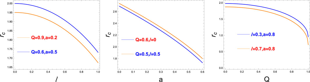
FIGURE 1. Variation of radii of the photon sphere for charged, rotating Kerr–Newman black-bounce metrics for various values of (a, Q, l). In the leftmost figure, we vary l keeping a and Q fixed. In the middle figure, we vary a keeping l and Q, and in the rightmost figure, we vary Q keeping a and l [120].

FIGURE 2

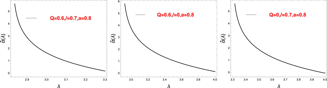
FIGURE 2. Variation of the deflection angle $\widehat{\alpha }$ with respect to the impact parameter λ for fixed values of Q, l, a [120].

4.4 Observational signature in the strong deflection limit

Now, we will discuss some observational consequences. The first step for this is to relate the deflection angle and the angular radius of the Einstein ring. This is performed by using a lens equation. In this paper, we will use the following lens equation [148]:

$\beta =\theta -\frac{{\mathit{D}}_{\mathit{L}\mathit{S}}}{{\mathit{D}}_{\mathit{O}\mathit{S}}}\mathrm{\Delta }{\alpha }_n,$(4.26)

where

${\mathit{D}}_{\mathit{O}\mathit{S}}={\mathit{D}}_{\mathit{O}\mathit{L}}+{\mathit{D}}_{\mathit{L}\mathit{S}}.$

Also, β is the angular separation between the source and the lens. D_LS, D_OS, D_OL are the distances between the lens to the source, the observer to the source, and the observer to the lens, respectively. Finally,

$\mathrm{\Delta }{\alpha }_n=\widehat{\alpha }\left(\theta \right)-2n\pi .$

The angular separation between the lens and the n^th image can be written as follows:

${\theta }_n={\theta }_n^0+\mathrm{\Delta }{\theta }_n,$

where ${\theta }_n^0$ is the angular separation between the n image and the lens when the extra deflection angle (Δθ_n) over 2nπ is negligible.

For the perfect alignment, that is, when β = 0 and assuming $\mathrm{\Delta }{\theta }_n\ll {\theta }_n^0$, the angular separation (angular radius) can be written as [79]

${\theta }_n^{\mathit{Einstein}}=\frac{{\lambda }_c}{{\mathit{D}}_{\mathit{O}\mathit{L}}}\left[1+\exp \left(\frac{\bar{b}}{\bar{a}}-\frac{2n\pi }{\bar{a}}\right)\right].$(4.27)

n = 1 corresponds to the outermost Einstein ring. Following [120], we plot some of these rings for different values of Q, a and l in Figure 3.

FIGURE 3

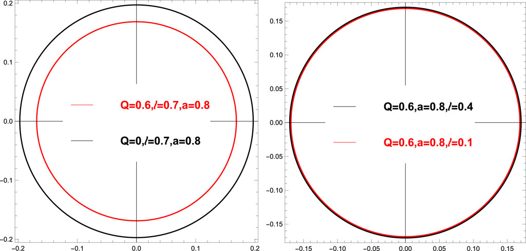
FIGURE 3. Polar plots showing the angular radius θ₁ for different Q, l, a values [120].

From the leftmost plot in Figure 3, we can conclude that as the charge of the black hole Q increases (for fixed l and a), the radii of the ring decrease. On the other hand, the effect of changing l (for fixed a and Q) on the ring radius is negligible. This is evident from the rightmost plot in Figure 3.

To make this observation more concrete, we carry out a detailed study, as shown in Tables 1, 2. Some of the values provided in (1) and (2) are reproduced from [120]. We have listed some values regarding the representative percentage change in the angular radius of the outermost Einstein rings with respect to Q (for fixed a and l) and l (for fixed a and Q) in Tables 1, 2, respectively. These values corroborate perfectly the conclusion drawn previously.

TABLE 1

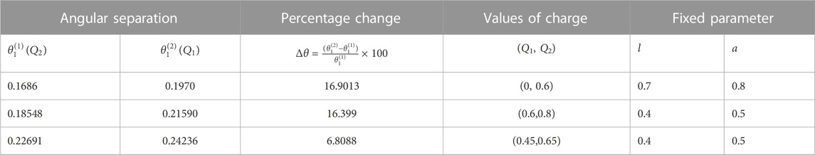
TABLE 1. Percentage change in the angular radius of the first Einstein ring for different values of charge Q for fixed a and l. Some of the numerical values presented here are reproduced from [120].

TABLE 2

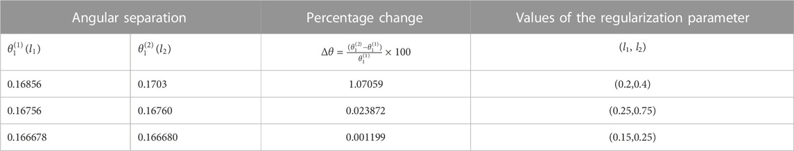
TABLE 2. Percentage change in the angular radius of the first Einstein ring for different values of the regularization parameter l for a = 0.8 and Q = 0.6. Some of the numerical values presented here are reproduced from [120].

Before closing this section, a few comments regarding possible avenues to constraints on the spacetime parameters should be in order, utilizing observational data. One of the ways is to look into the ratio of mass to distance, the mass being the mass of the central object (e.g., Sagittarius A*), which is around 4.4 × 10⁶M_⊙ and its distance being 8.5 kpc, the ratio turns out to be around 2.4734 × 10⁻¹¹. One can use these data to provide the angular position of the relativistic images and the angular separation between the two Einstein rings. On the other hand, we can compute the angular separation of two successive Einstein rings from (4.27) for different values of n. Then, one can utilize it to build a parameter space for the spacetime parameters. Interested readers are referred to, for example, [107] for a more comprehensive discussion. In future detections, if one can better resolve the angular separation of various Einstein rings, we will get better constraints on the charge of the underlying black-bounce metric.

4.5 Results for non-equatorial lensing: Caustic points

In Section 3.5, we discussed about the non-equatorial lensing for the Kerr–Newman black hole. For this case also, the analysis would be the same. The only difference is that the scaling factor ω(r) will be the function of the regularization parameter l apart from Q and a.

$\omega \left(r\right)=\bar{\lambda }\frac{a^2+\sqrt{r^2+l^2}\left(\sqrt{r^2+l^2}-2\right)}{\sqrt{r^2+l^2}\left(2a+\lambda \left(\sqrt{r^2+l^2}-2\right)\right)+Q^2\left(\lambda -a\right)},$(4.28)

with $\bar{\lambda }=\sqrt{{\lambda }^2-a^2}$.

Next, we show how the angular radius of the first Einstein ring depends on Q and l in Figure 4 following [120]. It is evident from Figure 4 that the dependence of the angular radius on the charge parameter (Q) of the black-bounce metric is significantly more than that on the regularization parameter (l) similar to the case of equatorial lensing.

FIGURE 4

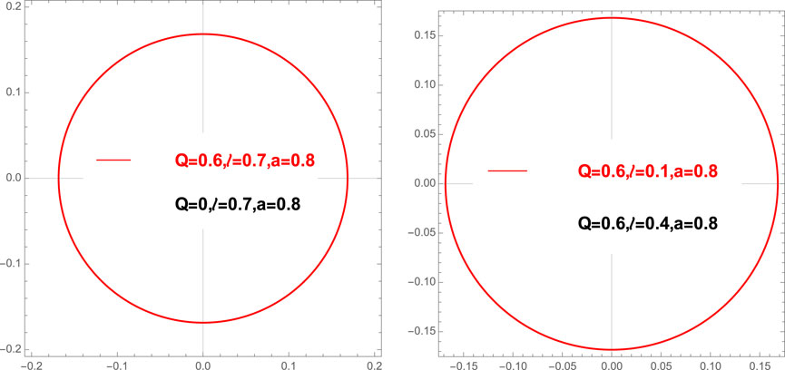
FIGURE 4. Polar plots showing the angular radius θ₁ for different Q, l, a values [120].

In Table 3, we investigate the variation of the second caustic point with respect to Q for fixed l and a.

TABLE 3

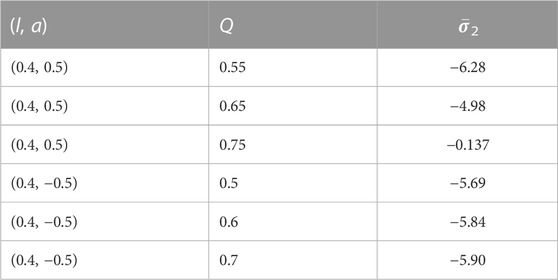
TABLE 3. Angular position of the second caustic point for different values of Q. The first three entities are for direct photons, and the last three are for retrograde photons. Some of the numerical values presented here are reproduced from [120].

Before closing this section, we further investigate the variation of the second caustic point with respect to l for fixed Q and a. It is demonstrated in Table 4. Comparing the values in Tables 3, 4, we can conclude that the change in caustic points for different Q and different l is not that robust [120].

TABLE 4

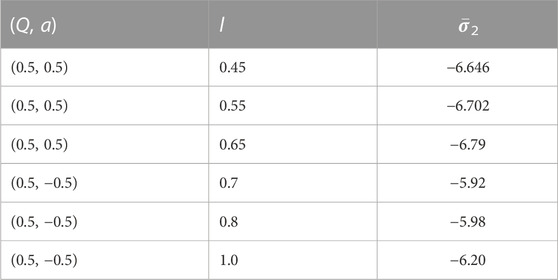
TABLE 4. Angular position of the second caustic point for different values of l. The first three entities are for direct photons, and the last three are for retrograde photons. Some of the numerical values presented here are reproduced from [120].

5 Conclusion

As mentioned earlier, gravitational lensing studies provide an excellent tool to provide insight into the structure of spacetime itself. In light of these advantages, this review provides a brief tour of the analytic methods used to calculate observables which can be measured. First, we review some facts about lensing in Schwarzschild geometry and observe the following points:

• The geodesics in this geometry are studied. As expected, owing to the symmetry of the spacetime itself, we have two constants of motion. Looking closely into the geodesic structures, we can find the location of the photon rings around them. Not only that, one can see that these photon rings located at 3M are unstable, and one can seek out some non-trivial physics once you deviate infinitesimally from this range.

• After we have understood how geodesics behave in such a geometry, we can calculate quantities using the equations at hand. A comprehensive and self-explanatory calculation is provided which gives an estimate of the deflection angle in terms of the central massive object responsible for this deflection. The contribution of this central massive object in the formula is through the mass of the object. There is also a contribution from an r_min term in the denominator which indirectly also depends on the metric structure around the central massive object. We have also listed down some salient features related to the calculation in the bullet points in the following (Eq. 2.15).

After giving a brief overview of the time delay suffered by these geodesics and also going on to calculate the diameter of the Einstein ring in this setup, we move on to a more general spacetime having extra rotation parameters. As expected, all the aforementioned observables will have a non-trivial rotation parameter-dependent term. The calculations are all in the strong deflection limit and analytical. We also consider a more general class of proposed solutions called black-bounce spacetimes, where there is an extra parameter involved as a deviation of the already known solutions in GR. We list the salient features of our findings as follows:

• We presented a method of calculating the deflection angle analytically by performing a perturbation in l. The results are given in terms of elliptic integrals of various kinds. Also, we have restricted ourselves to the equatorial plane while performing this analysis. We observe that for non-zero l, the value of the deflection angle for a fixed impact parameter decreases. Our calculation provides a general methodology to compute deflection angles analytically in a perturbative series. In future, it will be interesting to go beyond this small l expansion. This will require a thorough numerical analysis.

• Next, we study the strong deflection limit of the equatorial deflection angle. This has direct observational implications because it provides information about the Einstein rings. We can conclude that the effect of the charge (Q) on the size of the Einstein ring is much more pronounced than that of the regularization parameter (l) for a fixed value of spin parameter a. We discovered that decreasing the charge (Q) considerably increases the ring’s size. This observation remained the same even when we computed the ring’s radius for a small polar inclination.

• Furthermore, we extend our analysis for non-equatorial lensing. This enables us to compute the location of the caustic points. We again observed that the effect of the charge (Q) on the position of caustic points is more pronounced than the regularization parameter (l). Again, one can apply this method to different black hole spacetimes to obtain an exact analytical expression. The study of non-equatorial lensing presented in this review assumes a small inclination angle. Again, it will be interesting to go beyond this regime.

Another interesting direction we could not include in this review is the analysis of the structure of the shadow. Interested readers are referred to this review [149] for more details about this topic. Analysis of the shadow structure complements the analysis of the Einstein ring, which is presented here. It provides further constraints on the different black hole parameters and various theories of gravity. Interested readers are again referred to [149] for relevant references for this.

The analysis of the deflection angle presented in this review can straightforwardly be repeated to other black-bounce spacetimes, for example, [150]. Finally, there are several other avenues which have been pursued recently in the context of strong deflection of light rays. One such thing is the study of multilevel images. This helps one to predict how much resolution is required to distinguish between different Einstein rings. One important aspect is also to study the two-point correlation function of intensity fluctuations on the photon ring, which result from the photon traveling through several orbits around the central object. This plays a significant role from the perspective of image analysis. This black-bounce metric might be subject to these studies along the lines of [151]. These investigations will support our efforts to communicate with plausible astrophysical settings.

Author contributions

All authors listed have made a substantial, direct, and intellectual contribution to the work and approved it for publication.

Funding

Research of AC was supported by the Prime Minister’s Research Fellowship (PMRF-192002-1174) of Government of India. AB was supported by the Mathematical Research Impact Centric Support Grant (MTR/2021/000490) by the Department of Science and Technology Science and Engineering Research Board (India) and the Relevant Research Project grant (202011BRE03RP06633-BRNS) by the Board of Research in Nuclear Sciences (BRNS), Department of Atomic Energy (DAE), India.

Conflict of interest

The authors declare that the research was conducted in the absence of any commercial or financial relationships that could be construed as a potential conflict of interest.

Publisher’s note

All claims expressed in this article are solely those of the authors and do not necessarily represent those of their affiliated organizations, or those of the publisher, the editors, and the reviewers. Any product that may be evaluated in this article, or claim that may be made by its manufacturer, is not guaranteed or endorsed by the publisher.

Footnotes

¹This list is by no means exhaustive. Interested readers are referred to this review [24] and citations there for more details.

²Again, this list is by no means exhaustive. Interested readers are referred to the references and citations of these papers.

³For deflection of the massive particle, one needs to consider time-like trajectories given by $g_{\mu \nu }{\dot{x}}^{\mu }{\dot{x}}^{\nu }=-1$.

References

1. Dyson FW, Eddington AS, Davidson C. A determination of the deflection of light by the sun’s gravitational field, from observations made at the total eclipse of may 29, 1919. Phil Trans Roy Soc Lond A (1920) 220:291–333.

Google Scholar

2. Carroll SM. Lecture notes on general relativity (1997). gr-qc/9712019.

Google Scholar

3. Jackiw R, Pi S-Y. Chern-Simons modification of general relativity. Phys Rev D (2003) 68:104012. doi:10.1103/physrevd.68.104012

CrossRef Full Text | Google Scholar

4. Kanti P, Mavromatos NE, Rizos J, Tamvakis K, Winstanley E. Dilatonic black holes in higher curvature string gravity. Phys Rev D (1996) 54:5049–58. [hep-th/9511071]. doi:10.1103/physrevd.54.5049

CrossRef Full Text | Google Scholar

5. Horndeski GW. Second-order scalar-tensor field equations in a four-dimensional space. Int J Theor Phys (1974) 10:363–84. doi:10.1007/bf01807638

CrossRef Full Text | Google Scholar

6. Eling C, Jacobson T, Mattingly D. Einstein-Aether theory. In: Deserfest: A celebration of the life and works of stanley deser (2004). p. 163–79. 10, 2004.gr-qc/0410001.

Google Scholar

7. Moffat JW. Black holes in modified gravity (MOG). Eur Phys J C (2015) 75(4):175. [1412.5424]. doi:10.1140/epjc/s10052-015-3405-x

CrossRef Full Text | Google Scholar

8. Gao X. Unifying framework for scalar-tensor theories of gravity. Phys Rev D (2014) 90:081501. [1406.0822]. doi:10.1103/physrevd.90.081501

CrossRef Full Text | Google Scholar

9. Gao X, Yamaguchi M, Yoshida D. Higher derivative scalar-tensor theory through a non-dynamical scalar field. JCAP (2019) 03:006. [1810.07434]. doi:10.1088/1475-7516/2019/03/006

CrossRef Full Text | Google Scholar

10. Gross DJ, Witten E. Superstring modifications of Einstein’s equations. Nucl Phys B (1986) 277:1–10. doi:10.1016/0550-3213(86)90429-3

CrossRef Full Text | Google Scholar

11. Gross DJ, Sloan JH. The quartic effective action for the heterotic string. Nucl Phys B (1987) 291:41–89. doi:10.1016/0550-3213(87)90465-2

CrossRef Full Text | Google Scholar

12. de Roo M, Suelmann H, Wiedemann A. The Supersymmetric effective action of the heterotic string in ten-dimensions. Nucl Phys B (1993) 405:326–66. [hep-th/9210099]. doi:10.1016/0550-3213(93)90550-9

CrossRef Full Text | Google Scholar

13. Lovelock D. The Einstein tensor and its generalizations. J Math Phys (1971) 12:498–501. doi:10.1063/1.1665613

CrossRef Full Text | Google Scholar

14. Lovelock D. The four-dimensionality of space and the einstein tensor. J Math Phys (1972) 13:874–6. doi:10.1063/1.1666069

CrossRef Full Text | Google Scholar

15. Lodge OJ. Gravitation and light. Nature (1919) 104:354. doi:10.1038/104354a0

CrossRef Full Text | Google Scholar

16. Chwolson O. Traité de Physique, 5 vols. Paris: Hermann (1906-1919).

Google Scholar

17. Chwolson O, Chwolson O. Astr Nach (1924) 221:329–30.

CrossRef Full Text

18. Hewitt JN, Turner EL, Schneider DP, Burke BF, Langston GI, Lawrence CR. Unusual radio source MG1131+0456: A possible einstein ring. Nature (1988) 333:537–40. doi:10.1038/333537a0

CrossRef Full Text | Google Scholar

19. Hewitt JN, Turner EL, Lawrence CR, Schneider DP, Brody JP. A gravitational lens candidate with an unusually red optical counterpart. Astron J (1992) 104:968. doi:10.1086/116290

CrossRef Full Text | Google Scholar

20. Hewitt JN, Chen GH, Messier MD. Variability in the einstein ring gravitational lens MG 1131+0456. Astron J (1995) 109:1956. doi:10.1086/117421

CrossRef Full Text | Google Scholar

21. Hammer F, Le Fevre O, Angonin MC, Meylan G, Smette A, Surdej J, et al. 1131+0456: Discovery of the optical einstein ring with the NTT, Astron Astrophys 250 (1991) L5.

Google Scholar

22.James Webb Space Telescope Goddard Space Flight Center. James Webb space telescope goddard space flight center (2022). Available from: https://webb.nasa.gov/.

Google Scholar

23. Schneider P, Ehlers J, Falco EE. Gravitational lenses (1992).

Google Scholar

24. Perlick V. Gravitational lensing from a spacetime perspective (2010). 1010.3416.

Google Scholar

25. Wambsganss J. Gravitational lensing in astronomy. Living Rev Relativity (1998) 1:12. [astro-ph/9812021]. doi:10.12942/lrr-1998-12

CrossRef Full Text | Google Scholar

26.Event Horizon Telescope Collaboration, Akiyama K, Alberdi A, Alef W, Asada K, Azulay R, Baczko A-K, et al. First M87 event horizon telescope results. I. The shadow of the supermassive black hole. Astrophys J Lett (2019) 875:L1. [1906.11238].

Google Scholar

27.Event Horizon Telescope Collaboration, Akiyama K, Alberdi A, Alef W, Asada K, Azulay R, Baczko A-K, et al. First M87 event horizon telescope results. II. Array and instrumentation. Astrophys J Lett (2019) 875(1):L2. [1906.11239].

Google Scholar

28.Event Horizon Telescope Collaboration, Akiyama K, Alberdi A, Alef W, Asada K, Azulay R, Baczko A-K, et al. First M87 event horizon telescope results. III. Data processing and calibration. Astrophys J Lett (2019) 875(1):L3. [1906.11240].

Google Scholar

29.Event Horizon Telescope Collaboration, Akiyama K, Alberdi A, Alef W, Asada K, Azulay R, Baczko A-K, et al. First M87 event horizon telescope results. IV. Imaging the central supermassive black hole. Astrophys J Lett (2019) 875(1):L4. [1906.11241].

Google Scholar

30.Event Horizon Telescope Collaboration, Akiyama K, Alberdi A, Alef W, Asada K, Azulay R, Baczko A-K, et al. First M87 event horizon telescope results. V. Physical origin of the asymmetric ring. Astrophys J Lett (2019) 875(1):L5. [1906.11242].

Google Scholar

31.Event Horizon Telescope Collaboration, Akiyama K, Alberdi A, Alef W, Asada K, Azulay R, Baczko A-K, et al. First M87 event horizon telescope results. VI. The shadow and mass of the central black hole. Astrophys J Lett (2019) 875(1):L6. [1906.11243].

Google Scholar

32.Event Horizon Telescope Collaboration, Akiyama K, Alberdi A, Alef W, Algaba JC, Anantua R, Asada K, et al. First Sagittarius A* event horizon telescope results. I. The shadow of the supermassive black hole in the center of the milky way. Astrophys J Lett (2022) 930(2):L12.

Google Scholar

33.Event Horizon Telescope Collaboration, Akiyama K, Alberdi A, Alef W, Algaba JC, Anantua R, Asada K, et al. First Sagittarius A* event horizon telescope results. II. EHT and multiwavelength observations, data processing, and calibration. Astrophys J Lett (2022) 930(2):L13.

Google Scholar

34.Event Horizon Telescope Collaboration, Akiyama K, Alberdi A, Alef W, Algaba JC, Anantua R, Asada K, et al. First Sagittarius A* event horizon telescope results. III. Imaging of the galactic center supermassive black hole. Astrophys J Lett (2022) 930(2):L14.

Google Scholar

35.Event Horizon Telescope Collaboration, Akiyama K, Alberdi A, Alef W, Algaba JC, Anantua R, Asada K, et al. First Sagittarius A* event horizon telescope results. IV. Variability, morphology, and black hole mass. Astrophys J Lett (2022) 930(2):L15.

Google Scholar

36.Event Horizon Telescope Collaboration, Akiyama K, Alberdi A, Alef W, Algaba JC, Anantua R, Asada K, et al. First Sagittarius A* event horizon telescope results. V. Testing astrophysical models of the galactic center black hole. Astrophys J Lett (2022) 930(2):L16.

Google Scholar

37.Event Horizon Telescope Collaboration, Akiyama K, Alberdi A, Alef W, Algaba JC, Anantua R, Asada K, et al. First Sagittarius A* event horizon telescope results. VI. Testing the black hole metric. Astrophys J Lett (2022) 930(2):L17.

Google Scholar

38.Event Horizon Telescope Collaboration, Kocherlakota P, Rezzolla L, Falcke H, Fromm MC, Kramer M, Mizuno Y, et al. Constraints on black-hole charges with the 2017 EHT observations of M87*. Phys Rev D (2021) 103(10):104047. [2105.09343].

Google Scholar

39.LIGO ScientificVirgo Collaboration, Abbott BP, Abbott R, Abbott TD, Abernathy MR, Acernese F, Ackley K, et al. Observation of gravitational waves from a binary black hole merger. Phys Rev Lett (2016) 116(6):061102. [1602.03837]. doi:10.1103/PhysRevLett.116.061102

PubMed Abstract | CrossRef Full Text | Google Scholar

40.LIGO ScientificVirgo Collaboration, Abbott BP, Abbott R, Abbott TD, Abernathy MR, Acernese F, Ackley K, et al. Properties of the binary black hole merger GW150914. Phys Rev Lett (2016) 116(24):241102. [1602.03840]. doi:10.1103/PhysRevLett.116.241102

PubMed Abstract | CrossRef Full Text | Google Scholar

41.LIGO ScientificVirgo Collaboration, Abbott BP, Abbott R, Abbott TD, Abernathy MR, Acernese F, Ackley K, et al. GW151226: Observation of gravitational waves from a 22-solar-mass binary black hole coalescence. Phys Rev Lett (2016) 116(24):241103. [1606.04855]. doi:10.1103/PhysRevLett.116.241103

PubMed Abstract | CrossRef Full Text | Google Scholar

42.LIGO ScientificVIRGO Collaboration, Abbott BP, Abbott R, Abbott TD, Acernese F, Ackley K, Adams C, et al. GW170104: Observation of a 50-solar-mass binary black hole coalescence at redshift 0.2. Phys Rev Lett 118 (2017), no. 22, 221101 [1706.01812], [Erratum: Phys.Rev.Lett. 121, 129901 (2018)].

PubMed Abstract | Google Scholar

43.LIGO ScientificKAGRAVIRGO Collaboration, Abbott R, Abbott TD, Abraham S, Acernese F, Ackley K, Adams C, et al. Observation of gravitational waves from two neutron star–black hole coalescences. Astrophys J Lett (2021) 915(1):L5. [2106.15163].

Google Scholar

44.KAGRA Collaboration, Kokeyama K. Observing the universe from underground gravitational wave telescope KAGRA. In: 3rd world summit on exploring the dark side of the universe (2020). p. 41–8.

Google Scholar

45.LIGO ScientificVirgo Collaboration, Abbott BP, Abbott R, Abbott TD, Acernese F, Ackley K, Adams C, et al. Tests of general relativity with the binary black hole signals from the LIGO-virgo catalog GWTC-1. Phys Rev D (2019) 100(10):104036. [1903.04467].

Google Scholar

46.LIGO ScientificVIRGOKAGRA Collaboration, Abbott R, Abe H, Acernese F, Ackley K, Adhikari N, Adhikari RX, et al. Tests of general relativity with GWTC-3 (2021). 2112.06861.

Google Scholar

47. Psaltis D, Abbott R, Abe H, Acernese F, Ackley K, Adhikari N, et al. Testing general relativity with the event horizon telescope. Gen Rel Grav (2019) 51(10):137. [1806.09740]. doi:10.1007/s10714-019-2611-5

CrossRef Full Text | Google Scholar

48. Himwich E, Johnson MD, Lupsasca A, Strominger A. Universal polarimetric signatures of the black hole photon ring. Phys Rev D (2020) 101(8):084020. [2001.08750]. doi:10.1103/physrevd.101.084020

CrossRef Full Text | Google Scholar

49. Gralla SE. Can the EHT M87 results be used to test general relativity? Phys Rev D (2021) 103(2):024023. [2010.08557]. doi:10.1103/physrevd.103.024023

CrossRef Full Text | Google Scholar

50. Vagnozzi S, Roy R, Tsai YD, Visinelli L. Horizon-scale tests of gravity theories and fundamental physics from the Event Horizon Telescope image of Sagittarius A* (2022). 2205.07787.

Google Scholar

51. Völkel SH, Barausse E, Franchini N, Broderick AE. EHT tests of the strong-field regime of general relativity. Class Quant Grav (2021) 38(21):21LT01. [2011.06812]. doi:10.1088/1361-6382/ac27ed

CrossRef Full Text | Google Scholar

52. Bambi C, Freese K, Vagnozzi S, Visinelli L. Testing the rotational nature of the supermassive object M87* from the circularity and size of its first image. Phys Rev D (2019) 100(4):044057. [1904.12983]. doi:10.1103/physrevd.100.044057

CrossRef Full Text | Google Scholar

53. Vagnozzi S, Visinelli L. Hunting for extra dimensions in the shadow of M87*. Phys Rev D (2019) 100(2):024020. [1905.12421]. doi:10.1103/physrevd.100.024020

CrossRef Full Text | Google Scholar

54. Allahyari A, Khodadi M, Vagnozzi S, Mota DF. Magnetically charged black holes from non-linear electrodynamics and the Event Horizon Telescope. JCAP (2020) 02:003. [1912.08231]. doi:10.1088/1475-7516/2020/02/003

CrossRef Full Text | Google Scholar

55. Khodadi M, Allahyari A, Vagnozzi S, Mota DF. Black holes with scalar hair in light of the Event Horizon Telescope. JCAP (2020) 09:026. [2005.05992]. doi:10.1088/1475-7516/2020/09/026

CrossRef Full Text | Google Scholar

56. Cunha PVP, Herdeiro CAR, Radu E, Runarsson HF. Shadows of Kerr black holes with scalar hair. Phys Rev Lett (2015) 115(21):211102. [1509.00021]. doi:10.1103/physrevlett.115.211102

PubMed Abstract | CrossRef Full Text | Google Scholar

57. Wang M, Chen S, Jing J. Shadow casted by a Konoplya-Zhidenko rotating non-Kerr black hole. JCAP (2017) 10:051. [1707.09451]. doi:10.1088/1475-7516/2017/10/051

CrossRef Full Text | Google Scholar

58. Younsi Z, Zhidenko A, Rezzolla L, Konoplya R, Mizuno Y. New method for shadow calculations: Application to parametrized axisymmetric black holes. Phys Rev D (2016) 94(8):084025. [1607.05767]. doi:10.1103/physrevd.94.084025

CrossRef Full Text | Google Scholar

59. Bisnovatyi-Kogan GS, Tsupko OY. Shadow of a black hole at cosmological distances. Phys Rev D (2018) 98(8):084020. [1805.03311]. doi:10.1103/physrevd.98.084020

CrossRef Full Text | Google Scholar

60. Banerjee I, Chakraborty S, SenGupta S. Silhouette of M87*: A new window to peek into the world of hidden dimensions. Phys Rev D (2020) 101(4):041301. [1909.09385]. doi:10.1103/physrevd.101.041301

CrossRef Full Text | Google Scholar

61. Tsupko OY, Bisnovatyi-Kogan GS. First analytical calculation of black hole shadow in McVittie metric. Int J Mod Phys D (2020) 29(09):2050062. [1912.07495]. doi:10.1142/s0218271820500625

CrossRef Full Text | Google Scholar

62. Tsupko OY, Fan Z, Bisnovatyi-Kogan GS. Black hole shadow as a standard ruler in cosmology. Class Quant Grav (2020) 37(6):065016. [1905.10509]. doi:10.1088/1361-6382/ab6f7d

CrossRef Full Text | Google Scholar

63. Mishra AK, Chakraborty S, Sarkar S. Understanding photon sphere and black hole shadow in dynamically evolving spacetimes. Phys Rev D (2019) 99(10):104080. [1903.06376]. doi:10.1103/physrevd.99.104080

CrossRef Full Text | Google Scholar

64. Vagnozzi S, Bambi C, Visinelli L. Concerns regarding the use of black hole shadows as standard rulers. Class Quant Grav (2020) 37(8):087001. [2001.02986]. doi:10.1088/1361-6382/ab7965

CrossRef Full Text | Google Scholar

65. Li P-C, Guo M, Chen B. Shadow of a spinning black hole in an expanding universe. Phys Rev D (2020) 101(8):084041. [2001.04231]. doi:10.1103/physrevd.101.084041

CrossRef Full Text | Google Scholar

66. Perlick V, Tsupko OY. Light propagation in a plasma on Kerr spacetime: Separation of the Hamilton-Jacobi equation and calculation of the shadow. Phys Rev D (2017) 95(10):104003. [1702.08768]. doi:10.1103/physrevd.95.104003

CrossRef Full Text | Google Scholar

67. Wei SW, Liu YX, Mann RB. Intrinsic curvature and topology of shadows in Kerr spacetime. Phys Rev D (2019) 99(4):041303. [1811.00047]. doi:10.1103/physrevd.99.041303

CrossRef Full Text | Google Scholar

68. Chowdhuri A, Bhattacharyya A. Shadow analysis for rotating black holes in the presence of plasma for an expanding universe. Phys Rev D (2021) 104(6):064039. [2012.12914]. doi:10.1103/physrevd.104.064039

CrossRef Full Text | Google Scholar

69. Papnoi U, Atamurotov F, Ghosh SG, Ahmedov B. Shadow of five-dimensional rotating Myers-Perry black hole. Phys Rev D (2014) 90(2):024073. [1407.0834]. doi:10.1103/physrevd.90.024073

CrossRef Full Text | Google Scholar

70. Lin F-L, Patel A, Pu HY. Black hole shadow with soft hair (2022). 2202.13559.

Google Scholar

71. Chandrasekhar S. The mathematical theory of black holes. Oxford classic texts in the physical sciences. Oxford: Oxford Univ. Press (2002).

Google Scholar

72. Adler SL, Virbhadra KS. Cosmological constant corrections to the photon sphere and black hole shadow radii (2022). 2205.04628.

Google Scholar

73. Virbhadra KS. Compactness of supermassive dark objects at galactic centers (2022). 2204.01792.

Google Scholar

74. Roy R, Vagnozzi S, Visinelli L. Superradiance evolution of black hole shadows revisited. Phys Rev D (2022) 105(8):083002. [2112.06932]. doi:10.1103/physrevd.105.083002

CrossRef Full Text | Google Scholar

75. Chen Y, Roy R, Vagnozzi S, Visinelli L. Superradiant evolution of the shadow and photon ring of Sgr A* (2022). 2205.06238.

Google Scholar

76. Bozza V. Gravitational lensing in the strong field limit. Phys Rev D (2002) 66:103001. [gr-qc/0208075]. doi:10.1103/physrevd.66.103001

CrossRef Full Text | Google Scholar

77. Virbhadra KS, Ellis GFR. Schwarzschild black hole lensing. Phys Rev D (2000) 62:084003. [astro-ph/9904193]. doi:10.1103/physrevd.62.084003

CrossRef Full Text | Google Scholar

78. Frittelli S, Kling TP, Newman ET. Space-time perspective of Schwarzschild lensing. Phys Rev D (2000) 61:064021. [gr-qc/0001037]. doi:10.1103/physrevd.61.064021

CrossRef Full Text | Google Scholar

79. Bozza V. Quasiequatorial gravitational lensing by spinning black holes in the strong field limit. Phys Rev D (2003) 67:103006. [gr-qc/0210109]. doi:10.1103/physrevd.67.103006

CrossRef Full Text | Google Scholar

80. Bozza V. Comparison of approximate gravitational lens equations and a proposal for an improved new one. Phys Rev D (2008) 78:103005. [0807.3872]. doi:10.1103/physrevd.78.103005

CrossRef Full Text | Google Scholar

81. Einstein A. Lens-like action of a star by the deviation of light in the gravitational field. Science (1936) 84:506–7. doi:10.1126/science.84.2188.506

PubMed Abstract | CrossRef Full Text | Google Scholar

82. Eiroa EF, Sendra CM. Gravitational lensing by a regular black hole. Class Quant Grav (2011) 28:085008. [1011.2455]. doi:10.1088/0264-9381/28/8/085008

CrossRef Full Text | Google Scholar

83. Bin-Nun AY. Strong gravitational lensing by Sgr A*. Quant Grav (2011) 28:114003. [1011.5848]. doi:10.1088/0264-9381/28/11/114003

CrossRef Full Text | Google Scholar

84. Amarilla L, Eiroa EF, Giribet G. Null geodesics and shadow of a rotating black hole in extended Chern-Simons modified gravity. Phys Rev D (2010) 81:124045. [1005.0607]. doi:10.1103/physrevd.81.124045

CrossRef Full Text | Google Scholar

85. Stefanov IZ, Yazadjiev SS, Gyulchev GG. Connection between black-hole quasinormal modes and lensing in the strong deflection limit. Phys Rev Lett (2010) 104:251103. [1003.1609]. doi:10.1103/physrevlett.104.251103

PubMed Abstract | CrossRef Full Text | Google Scholar

86. Wei S-W, Liu YX, Fu CE, Yang K. Strong field limit analysis of gravitational lensing in Kerr-Taub-NUT spacetime. JCAP (2012) 10:053. [1104.0776]. doi:10.1088/1475-7516/2012/10/053

CrossRef Full Text | Google Scholar

87. Chen S, Liu Y, Jing J. Strong gravitational lensing in a squashed Kaluza-Klein Gödel black hole. Phys Rev D (2011) 83:124019. [1102.0086]. doi:10.1103/physrevd.83.124019

CrossRef Full Text | Google Scholar

88. Gyulchev GN, Stefanov IZ. Gravitational lensing by phantom black holes. Phys Rev D (2013) 87(6):063005. [1211.3458]. doi:10.1103/physrevd.87.063005

CrossRef Full Text | Google Scholar

89. Tsukamoto N, Harada T, Yajima K. Can we distinguish between black holes and wormholes by their Einstein ring systems? Phys Rev D (2012) 86:104062. [1207.0047]. doi:10.1103/physrevd.86.104062

CrossRef Full Text | Google Scholar

90. Sahu S, Patil M, Narasimha D, Joshi PS. Can strong gravitational lensing distinguish naked singularities from black holes? Phys Rev D (2012) 86:063010. [1206.3077]. doi:10.1103/physrevd.86.063010

CrossRef Full Text | Google Scholar

91. Chen S, Jing J. Strong gravitational lensing by a rotating non-Kerr compact object. Phys Rev D (2012) 85:124029. [1204.2468]. doi:10.1103/physrevd.85.124029

CrossRef Full Text | Google Scholar

92. Wei SW, Liu YX. Observing the shadow of Einstein-Maxwell-Dilaton-Axion black hole. JCAP (2013) 11:063. [1311.4251]. doi:10.1088/1475-7516/2013/11/063

CrossRef Full Text | Google Scholar

93. Atamurotov F, Abdujabbarov A, Ahmedov B. Shadow of rotating non-Kerr black hole. Phys Rev D (2013) 88(6):064004. doi:10.1103/physrevd.88.064004

CrossRef Full Text | Google Scholar

94. Eiroa EF, Sendra CM. Regular phantom black hole gravitational lensing. Phys Rev D (2013) 88(10):103007. [1308.5959]. doi:10.1103/physrevd.88.103007

CrossRef Full Text | Google Scholar

95. Wei SW, Yang K, Liu YX. Black hole solution and strong gravitational lensing in Eddington-inspired Born–Infeld gravity. Eur Phys J C (2015) 75:253. [1405.2178], [Erratum: Eur.Phys.J.C 75, 331 (2015)]. doi:10.1140/epjc/s10052-015-3469-7

CrossRef Full Text | Google Scholar

96. Tsukamoto N, Kitamura T, Nakajima K, Asada H. Gravitational lensing in Tangherlini spacetime in the weak gravitational field and the strong gravitational field. Phys Rev D (2014) 90(6):064043. [1402.6823]. doi:10.1103/physrevd.90.064043

CrossRef Full Text | Google Scholar

97. Liu X, Jia J, Yang N. Gravitational lensing of massive particles in Schwarzschild gravity. Class Quant Grav (2016) 33(17):175014. [1512.04037]. doi:10.1088/0264-9381/33/17/175014

CrossRef Full Text | Google Scholar

98. Wei SW, Liu YX, Fu CE. Null geodesics and gravitational lensing in a nonsingular spacetime. Adv High Energ Phys. (2015) 2015:1–11. [1510.02560]. doi:10.1155/2015/454217

CrossRef Full Text | Google Scholar

99. Sotani H, Miyamoto U. Strong gravitational lensing by an electrically charged black hole in Eddington-inspired Born-Infeld gravity. Phys Rev D (2015) 92(4):044052. [1508.03119]. doi:10.1103/physrevd.92.044052

CrossRef Full Text | Google Scholar

100. Bisnovatyi-Kogan GS, Tsupko OY. Gravitational lensing in plasmic medium. Plasma Phys Rep (2015) 41:562–81. [1507.08545]. doi:10.1134/s1063780x15070016

CrossRef Full Text | Google Scholar

101. Sharif M, Iftikhar S. Strong gravitational lensing in non-commutative wormholes. Astrophys Space Sci (2015) 357(1):85. doi:10.1007/s10509-015-2231-9

CrossRef Full Text | Google Scholar

102. Younas A, Hussain S, Jamil M, Bahamonde S. Strong gravitational lensing by kiselev black hole. Phys Rev D (2015) 92(8):084042. [1502.01676]. doi:10.1103/physrevd.92.084042

CrossRef Full Text | Google Scholar

103. Chen S, Jing J. Strong gravitational lensing for the photons coupled to Weyl tensor in a Schwarzschild black hole spacetime. JCAP (2015) 10:002. [1502.01088]. doi:10.1088/1475-7516/2015/10/002

CrossRef Full Text | Google Scholar

104. Schee J, Stuchlík Z, Ahmedov B, Abdujabbarov A, Toshmatov B. Gravitational lensing by regular black holes surrounded by plasma. Int J Mod Phys D (2017) 26(5):1741011. doi:10.1142/s0218271817410115

CrossRef Full Text | Google Scholar

105. Man J, Cheng H. Analytical discussion on strong gravitational lensing for a massive source with af(R)global monopole. Phys Rev D (2015) 92(2):024004. [1205.4857]. doi:10.1103/physrevd.92.024004

CrossRef Full Text | Google Scholar

106. Tsukamoto N. Deflection angle in the strong deflection limit in a general asymptotically flat, static, spherically symmetric spacetime. Phys Rev D (2017) 95(6):064035. [1612.08251]. doi:10.1103/physrevd.95.064035

CrossRef Full Text | Google Scholar

107. Wang S, Chen S, Jing J. Strong gravitational lensing by a Konoplya-Zhidenko rotating non-Kerr compact object. JCAP (2016) 11:020. [1609.00802]. doi:10.1088/1475-7516/2016/11/020

CrossRef Full Text | Google Scholar

108. Tsukamoto N. Strong deflection limit analysis and gravitational lensing of an Ellis wormhole. Phys Rev D (2016) 94(12):124001. [1607.07022]. doi:10.1103/physrevd.94.124001

CrossRef Full Text | Google Scholar

109. Zhao F, Tang J, He F. Gravitational lensing effects of a Reissner–Nordstrom–de Sitter black hole. Phys Rev D (2016) 93(12):123017. doi:10.1103/physrevd.93.123017

CrossRef Full Text | Google Scholar

110. Aldi GF, Bozza V. Relativistic iron lines in accretion disks: The contribution of higher order images in the strong deflection limit. JCAP (2017) 02:033. [1607.05365]. doi:10.1088/1475-7516/2017/02/033

CrossRef Full Text | Google Scholar

111. Lu X, Yang FW, Xie Y. Strong gravitational field time delay for photons coupled to Weyl tensor in a Schwarzschild black hole. Eur Phys J C (2016) 76(7):357. [1606.02932]. doi:10.1140/epjc/s10052-016-4218-2

CrossRef Full Text | Google Scholar

112. Cavalcanti RT, da Silva AG, da Rocha R. Strong deflection limit lensing effects in the minimal geometric deformation and Casadio–Fabbri–Mazzacurati solutions. Class Quant Grav (2016) 33(21):215007. [1605.01271]. doi:10.1088/0264-9381/33/21/215007

CrossRef Full Text | Google Scholar

113. Zhao S-S, Xie Y. Strong field gravitational lensing by a charged Galileon black hole. JCAP (2016) 07:007. [1603.00637]. doi:10.1088/1475-7516/2016/07/007

CrossRef Full Text | Google Scholar

114. Shaikh R, Kar S. Gravitational lensing by scalar-tensor wormholes and the energy conditions. Phys Rev D (2017) 96(4):044037. [1705.11008]. doi:10.1103/physrevd.96.044037

CrossRef Full Text | Google Scholar

115. Rahman M, Sen AA. Astrophysical signatures of black holes in generalized proca theories. Phys Rev D (2019) 99(2):024052. [1810.09200]. doi:10.1103/physrevd.99.024052

CrossRef Full Text | Google Scholar

116. Virbhadra KS. Distortions of images of Schwarzschild lensing (2022). 2204.01879.

Google Scholar

117. Hsieh T, Lee DS, Lin CY. Strong gravitational lensing by Kerr and Kerr-Newman black holes. Phys Rev D (2021) 103(10):104063. [2101.09008]. doi:10.1103/physrevd.103.104063

CrossRef Full Text | Google Scholar

118. Hsieh T, Lee DS, Lin CY. Gravitational time delay effects by Kerr and Kerr-Newman black holes in strong field limits. Phys Rev D (2021) 104(10):104013. [2108.05006]. doi:10.1103/physrevd.104.104013

CrossRef Full Text | Google Scholar

119. Edery A, Godin J. Second order Kerr deflection. Gen Rel Grav (2006) 38:1715–22. doi:10.1007/s10714-006-0347-5

CrossRef Full Text | Google Scholar

120. Ghosh S, Bhattacharyya A. Analytical study of gravitational lensing in Kerr-Newman black-bounce spacetime. JCAP (2022) 11:006. [2206.09954]. doi:10.1088/1475-7516/2022/11/006

CrossRef Full Text | Google Scholar

121. Balazs NL. Effect of a gravitational field, due to a rotating body, on the plane of polarization of an electromagnetic wave. Phys Rev (1958) 110:236–9. doi:10.1103/physrev.110.236

CrossRef Full Text | Google Scholar

122. Plebanski J. Electromagnetic waves in gravitational fields. Phys Rev (1960) 118:1396–408. doi:10.1103/physrev.118.1396

CrossRef Full Text | Google Scholar

123. Atkinson RD. Light delays near a relativistic star. Astron J (1969) 74:320. doi:10.1086/110813

CrossRef Full Text | Google Scholar

124. de Felice F. On the gravitational field acting as an optical medium. Gen Relativity Gravitation (1971) 2:347–57. doi:10.1007/bf00758153

CrossRef Full Text | Google Scholar

125. Mashhoon B. Scattering of electromagnetic radiation from a black hole. Phys Rev D (1973) 7:2807–14. doi:10.1103/physrevd.7.2807

CrossRef Full Text | Google Scholar

126. Mashhoon B. Influence of gravitation on the propagation of electromagnetic radiation. Phys Rev D (1975) 11:2679–84. doi:10.1103/physrevd.11.2679

CrossRef Full Text | Google Scholar

127. Fischbach E, Freeman BS. Second-order contribution to the gravitational deflection of light. Phys Rev D (1980) 22:2950–2. doi:10.1103/physrevd.22.2950

CrossRef Full Text | Google Scholar

128. Sereno M. Gravitational lensing in metric theories of gravity. Phys Rev D (2003) 67:064007. doi:10.1103/physrevd.67.064007

CrossRef Full Text | Google Scholar

129. Ye X-H, Lin Q. A Simple optical analysis of gravitational lensing. J Mod Opt (2008) 55:1119–26. [0704.3485]. doi:10.1080/09500340701618395

CrossRef Full Text | Google Scholar

130. Sen AK. A more exact expression for the gravitational deflection of light, derived using material medium approach. Astrophysics (2010) 53:560–9. doi:10.1007/s10511-010-9148-3

CrossRef Full Text | Google Scholar

131. Roy S, Sen AK. Trajectory of a light ray in Kerr field: A material medium approach. Astrophys Space Sci (2015) 360(1):23. [1408.3212]. doi:10.1007/s10509-015-2538-6

CrossRef Full Text | Google Scholar

132. Chakraborty S, Sen AK. Deflection of light due to rotating mass – A comparison among the results of different approaches. J Phys Conf Ser (2014) 481:012008. doi:10.1088/1742-6596/481/1/012008

CrossRef Full Text | Google Scholar

133. Chakraborty S, Sen AK. Light deflection in Kerr field for off-equatorial source (2015). 1504.03124.

Google Scholar

134. Simpson A, Visser M. Black-bounce to traversable wormhole. JCAP (2019) 02:042. [1812.07114]. doi:10.1088/1475-7516/2019/02/042

CrossRef Full Text | Google Scholar

135. Lobo FSN, Rodrigues ME, Silva MVDS, Simpson A, Visser M. Novel black-bounce spacetimes: Wormholes, regularity, energy conditions, and causal structure. Phys Rev D (2021) 103(8):084052. [2009.12057]. doi:10.1103/physrevd.103.084052

CrossRef Full Text | Google Scholar

136. Mazza J, Franzin E, Liberati S. A novel family of rotating black hole mimickers. JCAP (2021) 04:082. [2102.01105]. doi:10.1088/1475-7516/2021/04/082

CrossRef Full Text | Google Scholar

137. Franzin E, Liberati S, Mazza J, Simpson A, Visser M. Charged black-bounce spacetimes. JCAP (2021) 07:036. [2104.11376]. doi:10.1088/1475-7516/2021/07/036

CrossRef Full Text | Google Scholar

138. Tsukamoto N. Gravitational lensing in the Simpson-Visser black-bounce spacetime in a strong deflection limit. Phys Rev D (2021) 103(2):024033. [2011.03932]. doi:10.1103/physrevd.103.024033

CrossRef Full Text | Google Scholar

139. Nascimento JR, Petrov AY, Porfirio PJ, Soares AR. Gravitational lensing in black-bounce spacetimes. Phys Rev D (2020) 102(4):044021. [2005.13096]. doi:10.1103/physrevd.102.044021

CrossRef Full Text | Google Scholar

140. Guerrero M, Olmo GJ, Rubiera-Garcia D, Gómez DSC. Shadows and optical appearance of black bounces illuminated by a thin accretion disk. JCAP (2021) 08:036. [2105.15073]. doi:10.1088/1475-7516/2021/08/036

CrossRef Full Text | Google Scholar

141. Islam SU, Kumar J, Ghosh SG. Strong gravitational lensing by rotating Simpson-Visser black holes. JCAP (2021) 10:013. [2104.00696]. doi:10.1088/1475-7516/2021/10/013

CrossRef Full Text | Google Scholar

142. Will CM. Gravity: Newtonian, post-Newtonian, and general relativistic (2016). p. 9–72.

CrossRef Full Text | Google Scholar

143. Iyer SV, Hansen EC. Light’s bending angle in the equatorial plane of a Kerr black hole. Phys Rev D (2009) 80:124023. [0907.5352]. doi:10.1103/physrevd.80.124023

CrossRef Full Text | Google Scholar

144. Hsiao YW, Lee DS, Lin CY. Equatorial light bending around Kerr-Newman black holes. Phys Rev D (2020) 101(6):064070. [1910.04372]. doi:10.1103/physrevd.101.064070

CrossRef Full Text | Google Scholar

145. Claudel CM, Virbhadra KS, Ellis GFR. The Geometry of photon surfaces. J Math Phys (2001) 42:818–38. [gr-qc/0005050]. doi:10.1063/1.1308507

CrossRef Full Text | Google Scholar

146. Müller T. Einstein rings as a tool for estimating distances and the mass of a Schwarzschild black hole. Phys Rev D (2008) 77:124042. doi:10.1103/physrevd.77.124042

CrossRef Full Text | Google Scholar

147. Virbhadra KS. Relativistic images of Schwarzschild black hole lensing. Phys Rev D (2009) 79:083004. [0810.2109]. doi:10.1103/physrevd.79.083004

CrossRef Full Text | Google Scholar

148. Bozza V, Capozziello S, Iovane G, Scarpetta G. Strong field limit of black hole gravitational lensing. Gen Rel Grav (2001) 33:1535–48. [gr-qc/0102068]. doi:10.1023/a:1012292927358

CrossRef Full Text | Google Scholar

149. Perlick V, Tsupko OY. Calculating black hole shadows: Review of analytical studies. Phys Rept (2022) 947:1–39. [2105.07101]. doi:10.1016/j.physrep.2021.10.004

CrossRef Full Text | Google Scholar

150. Barrientos J, Cisterna A, Mora N, Viganò A. AdS-Taub-NUT spacetimes and exact black bounces with scalar hair. Phys Rev D (2022) 106(2):024038. [2202.06706]. doi:10.1103/physrevd.106.024038

CrossRef Full Text | Google Scholar

151. Hadar S, Johnson MD, Lupsasca A, Wong GN. Photon ring autocorrelations. Phys Rev D (2021) 103(10):104038. [2010.03683]. doi:10.1103/physrevd.103.104038

CrossRef Full Text | Google Scholar

Appendix A: Details of the computation of the deflection angle for Kerr–Newman spacetime

Here, we give details of computing the integral mentioned in (3.16). First, we rewrite B(u) in the factorized form.

$B\left(u\right)=-Q^2{\left(1-w\right)}^2\left(u-u_1\right)\left(u-u_2\right)\left(u-u_3\right)\left(u-u_4\right),(\mathrm{A1})$

where

$u_1=\frac{X_1-2m-X_2}{4m{r}_0},(\mathrm{A2})$

$u_2=\frac{1}{r_0},(\mathrm{A3})$

$u_3=\frac{X_1-2m+X_2}{4m{r}_0},(\mathrm{A4})$

$u_4=\frac{2m}{Q^2}-\frac{X_1}{2m{r}_0}.(\mathrm{A5})$

Then, by choosing the constants X₁ and X₂, we can write down the roots in the following order: u₁ < u₂ < u₃ < u₄. Here, the positive roots are u₂, u₃, u₄, while the negative root is u₁. Then, we substitute Eqs A2–A5 into (A1) and compare it with the coefficients of u₀, u₂, u₃, u₄ in (3.14). This way, we can eventually extract the roots. That gives [144]

$\begin{array}{cc}\hfill & Q^2\left[X_2^2-\left(X_1-2m\right)\left(X_1+6m\right)+4X_1^2\right]=16m^2{r}_0\left(X_1-r_0\frac{1+\omega }{1-\omega }\right),\hfill \\ \hfill & X_2^2-{\left(X_1^2-2m\right)}^2=\frac{8m\left(X_1-2m\right)\left(Q^2{X}_1-4m^2{r}_0\right)}{Q^2\left(X_1-2m\right)-4m^2{r}_0},\hfill \\ \hfill & \left[X_2^2-{\left(X_1^2-2m\right)}^2\right]\left(\frac{1}{8m{r}_0^3}-\frac{Q^2{X}_1}{32m^3{r}_0^4}\right)=\frac{1}{{\lambda }^2{\left(1-\omega \right)}^2}.\hfill \end{array}(\mathrm{A6})$

Combining the first and second equation of (A6), we obtain the equation for X₁, which is given by

$\begin{array}{cc}\hfill & \frac{Q^2}{2m}{X}_1^3-\left(Q^2+4m{r}_0\right)X_1^2+\left(4m^2{r}_0+2m{Q}^2+\frac{8m^3{r}_0^2}{Q^2}+\frac{2m{r}_0^2\left(1+\omega \right)}{\left(1-\omega \right)}\right)X_1\hfill \\ \hfill & =4m^2{Q}^2+\frac{4m^2{r}_0^2\left(1+\omega \right)}{\left(1-\omega \right)}+\frac{8m^2{r}_0^3\left(1+\omega \right)}{Q^2\left(1-\omega \right)}.\hfill \end{array}(\mathrm{A7})$

Eq. A7 can be exactly solved. The positive real root X₁(m, ω, Q, r₀) turns out to be the one mentioned in (3.19) of Section 3.3.

From (3.20), one can easily check that when Q becomes zero, δ becomes π. In that limit, (3.19) can be written as follows:

$X_1\left(m,\omega ,Q=0,r_0\right)=r_0\frac{1+\omega }{1-\omega }.(\mathrm{A8})$

It then exactly reproduces the result for the Kerr black hole [143]. Furthermore, we can reproduce the result for the Reissner–Nordstrom black hole in the limit, a = 0, and the root of the equation (A7) then reduces to

$X_1\left(m,Q,\omega =1,r_c\right)={\left.2m\left(\frac{2m{r}_0}{Q^2}-1\right)\right|}_{r_c},(\mathrm{A9})$

where r_c is defined in (3.11), and the result (A9) matches with the result of [144].

Now, we try to factorize the remaining part of the integrand of (3.16). We obtain

$\frac{1-2mu\left(1-\omega \right)+Q^2{u}^2\left(1-\omega \right)}{1-2mu+\left(a^2+Q^2\right)u^2}=\frac{G_{+}}{u_{+}-u}+\frac{G_{-}}{u_{-}-u}+\frac{G_{Q+}u}{u_{+}-u}+\frac{G_{Q-}u}{u_{-}-u},(\mathrm{A10})$

where

$u_{\pm }=\frac{m\pm \sqrt{m^2-\left(a^2+Q^2\right)}}{a^2+Q^2}.(\mathrm{A11})$

G₋, G₊, G_Q+, G_Q− are defined in (3.18) of Section 3.3. Also, we can easily see from (A11) u_± are positive.