Scientific debate on human migration: ethics, challenges, and solutions

Introduction: In recent years, we witnessed increasing numbers of migrants worldwide owing to famine, poverty, regional conflicts, etc. Efforts by the United Nations and various organizations to help these migrants are hampered by rising anti-migrant sentiments and xenophobic rhetoric in many parts of the world. To arrive at win-win solutions that benefit both natives and migrants, we must discuss the migration problem objectively and scientifically. To do this, we must first resolve the paradox in our understanding of human migration (widely touted as good) vis-a-vis biological invasion (generally regarded as bad).

Method: Suspecting that the two similar phenomena are more complex than we think, we reviewed and synthesized the disjoint literatures on human migration and biological invasion in recent times, and that on the human diaspora and human-aided dispersal of plants and animals in our pre-historic past. We then developed models of niche-niche interactions to simulate isolated ecosystems and communities, as well as those experiencing invasions from non-native populations.

Results: In this paper, we simulated four invasion mechanisms on a star network: the direct introduction of a non-native population into existing periphery or core niches, or the non-native population first creating its own niche, which is thereafter attached to the periphery or core of the community. We found that periphery invasions can fail, i.e., the non-native population eventually disappears. When periphery invasion is successful, we found that there is little or no harm to the ecosystem or community. On the other hand, core invasion is always catastrophic, where the non-native population establishes itself at the expense of most or all of the native populations. For niche attachments, whether to the periphery or to the core, we found native and non-native populations coexisting in the end, sometimes with increased diversities.

Discussion: Our results provide promising new insights and theoretical grounds for policymakers to discuss the ethics of immigration issues scientifically, and to ultimately discover win-win solutions for natives and migrants. The theoretical framework outlined in this paper can also be applied to the problem of introducing non-native biological species for economic gains, at acceptable ecological costs.

1 Introduction

Since Russia invaded Ukraine on 24 February 2022, 7.1 million people have fled the war [1], whereas 11 years into the Syrian Civil War, 6.8 million people had left the country (most of them to neighbouring Middle East countries, and about 1 million to Europe [2, 3]). Over in the United States (US), there is a new wave of illegal border crossings, with 1.7 million reported in 2021 [4] and 1.8 million reported in 2022 to date [5]. Some of these displaced peoples might return to their homes eventually, but others will choose to remain where they have settled.

Globally, the International Organization on Migration (IOM) reported in June 2019 that there were 272 million international migrants, nearly two-thirds of which were labour migrants [6]. As we can see from Figure 1, this number has been increasing over the years. In the same report, international migrants in 2019 made up 3.5 per cent of the world’s population, compared to 2.8 per cent in 2000, and 2.3 per cent in 1980. Unlike domestic migration, which is guaranteed by the 1948 United Nations (UN)’s universal declaration as a human right, the freedom to migrate across national boundaries is still work in progress. The latest consensus amongst governments is the non-binding Global Compact for Migration, first raised in 2016, concluded in 2018, and formally endorsed by the UN General Assembly on 19 December 2018 [7].

FIGURE 1

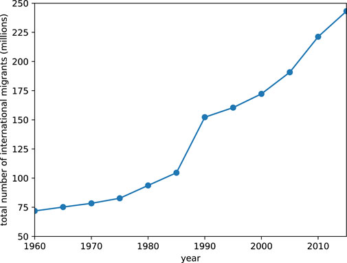
FIGURE 1. The global total number of international migrants between 1960 and 2015.

Legal international migration is not enshrined as a fundamental human right, because sovereign states do not feel comfortable letting in large numbers of foreign-born persons at any given time. This creates a paradox, since many believe that immigration is good, because it increases diversity, and because migrants tend to be more hardworking [8]. On the other hand, we find the opposite claim in the analogous situation of biological invasion, with ecologists decrying the effects of invasive species outperforming native species, leading to the latter’s demise.

In some sense, the ecologists’ claim seems more compelling, since they track both the invasive population, as well as native populations in their studies. In contrast, for human migration, advocates mostly consider the migration issue from the perspective of the migrants. Adverse effects on local populations are not highlighted. However, we should not immediately assume that one party is correct, while the other is wrong. Fundamentally, how can the outcomes of biological invasions and human migration be so different, when their dynamics are highly similar? Perhaps there are subtle differences between the two problems, and if we can understand these, we can use the desirable features of one to alleviate the ills of the other.

In this paper, we shall assume that both beneficial and deleterious invasions are possible, depending on the detailed conditions. That is to say, in addition to an invasive species wreaking havoc on a native ecosystem, we can also have the invasive species multiplying alongside native populations that continue to do well, or better. More precisely, we suspect that the diversity of a system can increase after an invasion, if the conditions are right. These insights would allow policymakers and governments to design migration policies that benefit native workers and societies, in an age of increasing migration worldwide due to globalization and regional conflicts.

To do so, we will first review in Section 2 the social science literature on immigration (the good), and the ecology literature on introduced species (the bad), to identify the key elements necessary to build common models. Thereafter, we will go on to review the archaeology literature on human and biological dispersals (the ugly), which frequently occurred together in our past. After synthesizing these disparate literatures, we realized that the relevant modelling framework to employ for comparative studies is that of niches (ecological, cultural, technological, and innovation) and their interactions. We review this literature in Section 3, before introducing our own niche-niche interaction models. In Section 4, we simulate our models for isolated ecosystems and communities under two classes of situations. In the first class of situations, which apply to both human migration and biological invasion, we directly introduce the invasive species into an existing niche. In the second class of situations, which apply only to human migration, we allow the invading population to create its own niche, before this niche is attached to the native community. In Section 5, we compare our simulation results, and discuss how they might be made more compelling or more realistic, and how they might inform immigration policies. In Section 6, we conclude.

2 Literature review

2.1 Human migration (good)

Human migration is the movement of people from one region (called the region/country of origin) to another region (called the host region/country). This movement can be temporary, where migrants return to their regions of origin, or permanent, where migrants and their future generations settle down permanently in the host region. Migration can occur within a country (domestic), or between countries (international). The reasons for migration are myriad. People can do so to seek better economic opportunities or better environments for their offspring (pull factors). It can also be to escape from criminal or political violence and oppression (push factors). Migration can also be classified as voluntary or involuntary. In the latter, migrants are classified as refugees.

To navigate the contemporary scholarly literature on human migration, we start from the 2017 paper by Sirkeci, Cohen, and Privara surveying the most influential papers and authors in migration studies [9]. This list is objective, since the ranking is created based on citations obtained from the Google Scholar database. Within the 100 most cited works, the earliest was in the late 1800s [10, 11] and the early 1900s [12]. There was then a long lapse, before the literature exploded after 1985, to reach a high around the year 2000 (see Figure 2). Thereafter, the number of highly-cited works decreased. Putting aside the early works, and looking at the post-2000 publications by the most influential migration scholars, we find them accepting migration as an ongoing phenomenon, with their papers investigating specific issues related to migration, without pronouncing whether migration is desirable or not.

FIGURE 2

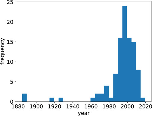
FIGURE 2. Histogram of the 100 most cited works in migration studies from Sirkeci, Cohen, and Privara [9].

Given this stance amongst leading scholars, it is difficult to understand why there is a one-sided opinion on migration as a good thing in traditional or social media. To clarify this, we surveyed opinions published in the media, starting with those who sing praises about human migration, before touching on those who object (and why they object). Wherever possible, we identify scholarly research these opinions are based off. Here, let us warn that opinion pieces do not cite references (opinions of previous writers), are not as comprehensively archived and indexed as scholarly publications, and hence we are likely to miss earlier articles (especially if they pre-date the Google search engine).

Amongst the many advocates of migration, we find international organizations such as the International Organization on Migration (IOM). The IOM’s views on migration are understandably positive, since it is an organization created to serve migrants. Their support for migration is first and foremost based on human rights, but IOM argued that there are also other benefits. Another international organization that leans positively on migration is the Organization for Economic Co-operation and Development (OECD), who urges the public to accept more open immigration policies [13]. The World Economic Forum also argues that meaningful policies must balance the longer-term economic benefits that immigration brings with local and short-term costs [14].

The greatest divide in opinions about immigration occur at the level of think tanks. Advocates of immigration includes the non-profit IZA Institute of Labour Economics based in Bonn, Germany [15], and the Center for Global Liberty and Prosperity in the CATO Institute [16], an American libertarian think tank with headquarters in Washington DC, founded in 1977 by private philanthropists. Opponents to immigration tend to be think tanks strongly influenced by colorful individuals. These include advocacy groups such as NumbersUSA, and the Center for Immigration Studies, who make their cases in the form of books [17]. Opponents of migration appear to be the minority.

2.2 Biological invasion (bad)

Biological invasions happen when an organism (the invasive species) arrives from its distant native habitat. This can happen as a result of human actions (also known as human dispersals), either deliberately or accidentally. The invasive species can also be transported by mammals, birds, insects, and plants. According to the 1996 book Biological Invasions by Williamson [18], the invasion process consists of a series of steps (or stages), including transport, establishment, spread, and impact. Others have proposed four different stages, i.e., arrival, establishment, spread, and adjustment [19, 20]. Henderson [21], on the other hand, proposed six stages of biological invasion, namely, introduction, establishment, naturalization, dispersal, population distribution, and invasive spread.

The impact caused by biological invasions can be harmful to our health or our economy. Economically, Pimentel et al. [22] estimated in 2005 that invasive species cause environmental damages and losses adding up to almost $120 billion per year in the United States Policy and management options differ at different stages of a biological invasion, but it has been recognized once an invasion has started, the efforts to reverse it will be enormous. Therefore, preventive steps for stopping biological invasions are deemed more effective. They include early detection, rapid response, and eradication before the invasive species spreads. This is why United States President Bill Clinton signed Executive Order 13,751 to deal with invasive species in 1999.

But how did the ecology community become fixated on biological invasions as bad? To understand this, we reviewed literature going back to the mid-1700s, when the deliberate transportation of plants and animals by humans was first documented. According to Chew [23], Pehr Kalm traveled to North America seeking new plants that might be brought back to Sweden and grown commercially for economic benefit. Thereafter in the 1800s, a host of botanists and zoologist (including Charles Darwin and Alfred Russell Wallace) went around documenting the distribution of the world’s biota, and brought samples back home with them. These data sets and collections laid the conceptual groundwork for the modern sciences of evolutionary biology as well as ecology in the 20th century. This was also when native and non-native species were first formally defined. However, in those days no one was of the opinion that the deliberate introduction of non-native species into various ecosystems for economic purposes was bad.

According to Cadotte [24], North American agricultural scientists in the middle of the 19th century started noticing the negative impacts of non-native species [25]. By the end of the 19th century, such commentaries became more common [26–28]. The notion that movements of species between ecosystems were bad was popularized by Charles Elton (who is considered the forefather of the field of biological invasions), who in 1958 wrote a book titled The Ecology of Invasions by Animals and Plants [29], and also coined the term invasive species. Over in Europe, ecologists were also becoming aware of the impacts of non-native species, but adopted a neutral attitude towards them. In particular, they deemed that the introduction of non-native species as just one of many factors that could cause the decline of native species [30]. In fact, 6 years after the publication of Elton’s book, the International Union of Biological Scientists (IUBS) held its first Biological Sciences Symposium in Asilomar, California, to facilitate discussions on “the kinds of evolutionary change which take place when organisms are introduced into new territories” amongst top geneticists, ecologists, taxonomists, and applied scientists working in the area of pest control [31].

The two views were balanced until 1980, when the Third International Conference on Mediterranean Ecosystems was held in Stellenbosch, South Africa. At this conference, the idea of biological invasions appealed to many participants, who deemed biological invasions to inevitably cause an impact to human societies and ecosystems if preventive and mitigation measures were not implemented promptly. Since then, books, conferences, and organizations on biological invasions have emerged. The issue was frequently discussed in mass media and also appeared in government policies in many countries. In short, the negative impressions towards non-native species may be attributed to Elton’s 1958 book, and also the 1980 South Africa conference. A complete account of the historical developments of this field can be found in Davis’s book on Invasion Biology [32].

2.3 Historical perspectives (ugly)

Human migration introduces new communities into an existing society with many established communities, whereas biological invasion involves new non-native species being introduced into an ecosystem with many existing species. Despite this similarity, human migration is largely considered as a positive change, while biological invasion is seen negatively. Between these two extremes, the real situation may actually be more complex. In fact, the history of human migration is effectively the history of our Homo sapiens species. Prehistorically, the earliest H. sapiens appeared to have occupied all of Africa about 150,000 years ago [33]. Around 70,000 years ago, humans started moving out of Africa into Asia and Europe [34, 35], across Australia, Asia, and Europe by 40,000 BCE [34, 35], and finally to the Americas 20,000 to 15,000 years ago [36]. Using historical records of human migration, McNeill classified them into four types, namely, (1) radical displacement via systematic exercise of force; (2) conquest of one population by another, (3) infiltration-type migration, and (4) slavery or exploitation-type migration [37]. Our modern definition of human migration is closest to types (3) and (4) (but less the slavery component).

Human migration of types 1 and 2 are rare in modern times, but common in our historic past. For example, nomads such as the Huns, Mongols, Turks, and many others raided each other in the Eurasian Steppe whenever opportunities presented themselves. The patterns of movements resulting from these skirmishes are classified as type 1 by McNeill. In contrast, human migration of type 2 occurs when a nomadic group encounters and overwhelms a farming society, and eventually the two communities become one [38–40]. However, itinerant peoples were not always raiders and conquerors. They also included merchants and traders, artisans with exotic skills, as well as scavengers and street food vendors. Their contact with local communities were welcomed, because they provided exclusive goods and services. Over time, these ‘strangers’ integrated into their host communities in what McNeill called type 3 human migration. Finally, there is type 4 human migration, which can be distinguished from type 3 by the involuntary displacement of large groups of peoples, either as slaves, or as cheap sources of labour.

As we can see, human migrations of types 1, 2, and 4 are clearly not acceptable today. If there are any good and desirable human migration, it must be of type 3. Besides the integration of various practical expertise into the host community through the assimilation of a small proportion of ‘outsiders’, human migration of this type also brought missionaries, teachers, medical and military experts and their knowledge to various communities. This infusion of knowledge increased the wealth of a host community without sacrificing social coherence. Certainly, this form of human migration plays an important role in shaping civilization as we know it today.

Moreover, the movements of human communities also resulted in the spread of plants and animals numerous times in pre-historic and historic times. The effects of these past movements were not documented, so it is difficult to assess what their social and ecological impacts were. In this survey of the literature, we do not aim to paint a comprehensive picture of all episodes of human migrations and the biological invasions that followed them, but to highlight the possibility that impacts of specific human migrations can be decidedly bad (the Eurasian Steppe example given above), and specific episodes where non-native species could be introduced without destroying or compensating host ecosystems. One example is the cultivation of rice, Oryza sativa. This plant was first domesticated in China between 13,500 and 8,200 years ago [41], then spread to the Korean Peninsula latest by 2,000 BCE [42], and to Japan by 1,000 BCE [43]. It was hypothesized that rice was domesticated a second time in India [44]. Today, rice is the staple food crop for more than 3.5 billion people around the world, and has historically supported the growth of human population.

Another example would be the pig, Sus scrofa, which was first domesticated from wild boars in Eastern Turkey 10,000 to 9,000 years ago [45, 46]. The pig was also independently domesticated in China between 10,000 and 8,000 years ago [47, 48]. From Eastern Turkey, domestic pigs spread to Northern Turkey [49], and throughout Europe by 5,500 BCE [50]. Thereafter, between 5,000 and 4,000 years ago, Austronesian-speaking rice agriculturalists from southern China migrated through Taiwan and Sundaland into southeast Asia and Oceania as well as westward to Madagascar, bringing with them domesticated pigs [51]. Today, the pig is an important source of animal protein for the world, but it is also one of the largest source of zoonotic diseases [52]. From the perspectives given above, the pig is thus both good (food) and bad (disease).

3 Exploratory modeling

3.1 Making the case for modeling

The immigration issue came to the fore during the 2016 United States Presidential Elections between Democrat candidate Hillary Clinton and Republican candidate Donald Trump. The debate grew so polarizing that in the September/October 2016 issue of Politico [53], an United States news outlet specializing in politics and policy, George Borjas explained how Donald Trump used half of his findings (that admitting large numbers of immigrants over many decades have led to lower wages and unemployment, especially for African and Hispanic Americans [54]) to justify tougher immigration policies and building the border wall, while Hillary Clinton used the other half of his findings (that both legal and illegal immigrants helped improve economic outcomes for everyone) to justify immigration policies to date. In fact, anti-immigrant sentiments are on the rise in many countries that accept foreign-born citizens. Unfortunately, contrary to calls for “a more balanced and evidence-based debate about migration, where the real facts are presented and discussed openly” [55], this is an ethical issue that cannot be settled with hard facts alone. We cannot keep telling the segments of our society negatively impacted by immigration that immigrants make the economic pie bigger, when these benefits do not actually go to them.

There is a similar set of considerations surrounding biological invasions by non-native species, and that is, who decides which non-natives species can or cannot be introduced. According to many ecologists, we would not introduce any non-native species at all. However, we also know from the history of humankind that our success on this planet was strongly influenced by our spreading of non-native plant and animal species. Given this backdrop, we argue that it is reasonable to measure the benefits of introducing non-native species into an ecosystem (or a foreign community into society), against the potential biodiversity loss (or cultural diversity loss) that these might produce. In this paper, we are not advocating for the cessation of all movements of human communities and non-native plant and animal species, but to suggest how we can debate the ethics of allowing some such movements, and at the same time barring or intervening in others.

While some might argue that such ethical discussions are beyond the realm of science, we believe the scientific approach can be the basis for such debates, by providing not just data and hard evidence, but also compelling narratives derived from quantitative models. In the real world, we can either shut out immigrants, or let them in. If we have chosen one path of action, we will never know what happens for other paths of action. Thus this is where modelling comes in. The biggest advantage that models can offer is for us to simulate both scenarios, and measure quantities we are interested in. More importantly, different immigration policies can be compared first through simulations, before their outcomes are put on the table for policy discussions. Ultimately, the policy with the best economic outcome is not automatically selected, because we must also decide whether its social cost is acceptable. In the end, we may opt for a compromise, and go with a policy with reduced economic benefits, but whose social cost we decide that we are able to bear.

We proceed to describe a common modelling framework for human migration and biological invasions, because there are strong similarities between the two phenomena. Could it be that human migration can also be bad? Or perhaps the introduction of non-native species sometimes good? To find answers to these questions, we need to first use the same performance metric, instead of using economic benefits for one, and biodiversity for the other. To quantify diversity, it is customary to use the entropy function $S\left[\overrightarrow{p}=\left(p_1,\dots ,p_i,\dots ,p_N\right)\right]=-{\sum }_{i=1}^N{p}_i\log p_i$. For example, if we have $N$ communities that are equally represented, then the probability of finding an individual from a given community $i$ would be $p_i=1/N$. Such a society/ecosystem would have entropy $S={\sum }_{i=1}^N\frac{\log N}{N}=\log N$, which is the maximum possible for a system with $N$ communities. In contrast, if the first community has overwhelmingly many individuals, while the other communities are represented by a few individuals, then $S\approx 0$. When we go from a society or ecosystem with $N$ communities to one with $N+1$ communities, we ought to compare $S_{N+1}$ against $S_N$. Depending on the detail distribution $\overrightarrow{p}=\left\{p_i\right\}$, $S_{N+1}$ is not automatically larger than $S_N$.

3.2 Our model of interacting niches

In the Supplementary Material, we reviewed the literatures on ecological and evolutionary models of niches, as well as their applications to culture, technology and innovation. In the former, we find the work by May dealing with many interacting species exploiting a single resource type distributed in space [56]. For the ecosystem to be stable, May argued that the distributions of species will eventually become non-overlapping. These can then be thought of as niches for the different species. In the latter, Laland et al. [57] investigated how a single species’ fitness is determined by how strongly it modifies its environment with an unspecified number of resource types. They showed that niche construction allows even deleterious genes to persist in the population. In these literatures, the niche occupied by a species is a region of space (its habitat) that it has modified to favor itself (and disadvantage other species) and its offspring (inheritance). Since much of the debate on human migration and biological invasion is focused on introduced individuals and the first few generations of their offspring, we will not consider the effects of evolution in this paper. However, we do wish to explicitly model how introduced individuals interact with natives, by exploiting the native niches. This network of niches is implicitly assumed in May’s model, and in this paper we make their interactions explicit by writing down simple network models based on ordinary differential equations.

3.2.1 Operational definition of niches and niche-niche interactions

To arrive at such models, we must first recognize that niches (ecological or cultural) are fundamentally spatial in character, as illustrated in Figure 3A, where we divide the local environment into a spatial grid. Resources of multiple types are then distributed within these grid cells, and individuals from the red and green species can exploit these if they venture into the right grid cells. The information on which individuals exploit which cells can be represented as an exploration matrix shown in Figure 3B. We call the cells that an individual exploits its range, and the union of the ranges of all individuals of a species the collective range of the species. As we can see from Figure 3C, the collective range of the red species overlaps with the collective range of the green species. If we now perform co-clustering on the exploration matrix, to separate individuals and resource cells into non-overlapping groups, we get the niches (red and green) shown in Figure 3D. In this useful operational definition, niches are (i) collectively defined from data, (ii) non-overlapping, and (iii) smaller than the collective ranges of the species involved.

FIGURE 3

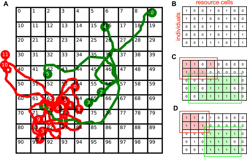
FIGURE 3. (A) Grid cells in a spatial landscape of resources, and the trajectories of individuals (numbered) from two species (red and green). (B) The exploration matrix $A$ whose rows are individuals from both species (the top two rows are from the red species, while the bottom three rows are from the green species), and whose columns are spatial grid cells (organized according to some initial ordering scheme). The element $A_{ij}=1$ if individual $i$ explored grid cell $j$, and $A_{ij}=0$ otherwise. (C) The exploration matrix $A$ after reordering the columns, so that the grid cells visited by red individuals are adjacent to each other, while grid cells visited by green individuals are adjacent to each other. The red rectangle indicates the collective range of the red species, while the green rectangle indicates the collective range of the green species. (D) Instead of showing the ranges of the two species, we can also show the niches of the two species. Here, the red rectangle indicates the niche occupied by the red species, while the green rectangle represents the niche occupied by the green species. The two rectangles are non-overlapping and can be discovered using community detection methods.

The next key ingredient of our model is the network representation of the ecosystem. As shown in Figure 3, the collective ranges of the red and green species overlap, which means that we find green individuals in the red niche (a region of space dominated by red individuals), and red individuals in the green niche (a region of space dominated by green individuals). If the two species compete for the same resources, the spatial boundaries of the red and green niches can change if green individuals become dominant in a red cell, or red individuals become dominant in a green cell. Therefore, the carrying capacity $K_i\left(t\right)$ of niche $i$ will depend on how well the $N_i\left(t\right)$ individuals from species $i$ compete with encroaching individuals (the number of which should be proportional to $N_j\left(t\right)$) from species $j$ for resources in niche $i$ at time $t$. In May’s work [56], $S$ species exploit the same resource, so if they are all close to each other, interactions between niches would be represented by the complete network shown in Figure 4A. In general, we know that ecosystems have nested structures as bipartite networks [58–61], which become unipartite core-periphery networks if we restrict the nodes to a single trophic level [62–65]. A simple network that has a core-periphery structure is the star network shown in Figure 4B.

FIGURE 4

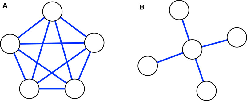
FIGURE 4. (A) A complete network of five niches. (B) A star network of five niches, with one core niche in the center, and four peripheral nodes linked to it. In this network representation, two niches that are linked will necessarily have populations that overlap spatially and share at least one common resource.

To distinguish between our models for biological invasion and human migration, we assume that in the former, niches are subjected to a constraint of the form

$\begin{array}{c}{K}_1\left(t\right)+K_2\left(t\right)+\dots +K_j\left(t\right)+\dots +K_S\left(t\right)={\displaystyle \sum _{j=1}^S}{K}_j\left(t\right)\le K_0,\end{array}(1)$

where $K_0$ is the total productivity of the environment, and $S$ is the total number of species. In general, $S$ need not start out being equal to the number of populated niches. If $S$ is fewer than the number of niches, we simply allow dormant niches (which have zero population and thus no dynamics). If we start out with more species than niches, then some species will have to compete for the same niches. We expect from the Lotka-Volterra model that only one species will survive in each niche in the long run.

3.2.2 Mathematical model in the absence of introduced species/communities

Based on the interactions shown in Figure 3 (with network representation in Figure 4), let us write down equations on how the niches change with time. We start by considering the interactions between niches $i$ and, with carrying capacities $K_i$ and $K_j$, supporting $N_i$ and $N_j$ individuals respectively. From the exploration matrix, we can not only determine $N_i$ and $N_j$, but also $n_{ji}$ (the number of individuals from species $i$ encroaching on niche $j$) and $n_{ij}$ (the number of individuals of species $j$ encroaching on niche $i$). The carrying capacity $K_i$ is then increased at a rate proportional to $n_{ji}$, and decreased at a rate proportional to $n_{ij}$. Since $n_{ji}$ is the number of individuals of species $i$ encroaching onto niche $j$, we expect $n_{ji}$ to be larger when $N_i$ is larger, and smaller if $N_i$ is smaller, i.e., $n_{ji}\propto N_i$. Similarly, $n_{ij}\propto N_j$, and we can write

$\begin{array}{c}\frac{d{K}_i}{dt}=+{\beta }_{ji}{N}_i-{\beta }_{ij}{N}_j,\end{array}(2)$

$\begin{array}{c}\frac{d{K}_j}{dt}=+{\beta }_{ij}{N}_j-{\beta }_{ji}{N}_i.\end{array}(3)$

In Eqs 2, 3, ${\beta }_{ji}$ and ${\beta }_{ij}$ are proportionality constants that tell us how effectively species $i$ exploit niche $j$, or species $j$ exploit niche $i$ respectively. We are also assuming at this point that the ecosystem consists only of species $i$ and $j$.

However, the proportionality constants ${\beta }_{ji}$ and ${\beta }_{ij}$ are still extensive quantities, as ${\beta }_{ji}$ depends on $K_j$, and ${\beta }_{ij}$ depends on $K_i$. In other words, species $i$’s exploitation of niche $j$ is more effective if $K_j$ is larger, and less effective if $K_j$ is smaller. The same is true for species $j$’s exploitation of niche $i$. Therefore, Eqs 2, 3 can be rewritten as

$\begin{array}{c}\frac{d{K}_i}{dt}=+{\gamma }_{ji}{K}_j{N}_i-{\gamma }_{ij}{K}_i{N}_j,\end{array}(4)$

$\begin{array}{c}\frac{d{K}_j}{dt}=+{\gamma }_{ij}{K}_i{N}_j-{\gamma }_{ji}{K}_j{N}_i,\end{array}(5)$

in terms of the intensive constants ${\gamma }_{ji}$ and ${\gamma }_{ij}$. For this ecosystem consisting of species $i$ and $j$, the model is complete once we specify how the populations $N_i$ and $N_j$ change with time. These can remain as the logistic growths

$\begin{array}{c}\frac{d{N}_i}{dt}={\mu }_i{N}_i\left(1-\frac{N_i}{K_i}\right),\end{array}(6)$

$\begin{array}{c}\frac{d{N}_j}{dt}={\mu }_j{N}_j\left(1-\frac{N_j}{K_j}\right),\end{array}(7)$

with time-dependent carrying capacities $K_i\left(t\right)$ and $K_j\left(t\right)$. Here ${\mu }_i$ and ${\mu }_j$ are the effective per capita growth rates of species $i$ and $j$.

If there are now $S$ species occupying $S$ interacting niches, we can then generalize Eq. 4 as

$\begin{array}{c}\frac{d{K}_i}{dt}=N_i{\displaystyle \sum _{j\ne i}^S}{\gamma }_{ji}{K}_j-K_i{\displaystyle \sum _{j\ne i}^S}{\gamma }_{ij}{N}_j,\end{array}(8)$

while Eq. 6 remains the same, for $i=1,\dots ,S$. This would constitute our full model, after specifying ${\mu }_i$ and ${\gamma }_{ij}$. If ${\gamma }_{ij}\ne 0$ for all $i$ and $j\ne i$, we have a weighted complete network of interacting niches. If only certain niches can interact, for example, those in a star network, we must have ${\gamma }_{ij}=0$ for some pairs of $i$ and $j\ne i$. Specifically, for the star network with five nodes shown in Figure 4B, if we always refer to the core as node $i=1$, the peripheral nodes as $i=2,3,4,5$, and keep only those ${\gamma }_{ij}\ne 0$, we can write Eq. 8 explicitly as

$\begin{array}{c}\frac{d{K}_1}{dt}=N_1\left({\gamma }_{21}{K}_2+{\gamma }_{31}{K}_3+{\gamma }_{41}{K}_4+{\gamma }_{51}{K}_5\right)-K_1\left({\gamma }_{12}{N}_2+{\gamma }_{13}{N}_3+{\gamma }_{14}{N}_4+{\gamma }_{15}{N}_5\right),\end{array}(\mathrm{9a})$

$\begin{array}{c}\frac{d{K}_2}{dt}={\gamma }_{12}{N}_2{K}_1-{\gamma }_{21}{N}_1{K}_2,\end{array}(\mathrm{9b})$

$\begin{array}{c}\frac{d{K}_3}{dt}={\gamma }_{13}{N}_3{K}_1-{\gamma }_{31}{N}_1{K}_3,\end{array}(\mathrm{9c})$

$\begin{array}{c}\frac{d{K}_4}{dt}={\gamma }_{14}{N}_4{K}_1-{\gamma }_{41}{N}_1{K}_4,\end{array}(\mathrm{9d})$

$\begin{array}{c}\frac{d{K}_5}{dt}={\gamma }_{15}{N}_5{K}_1-{\gamma }_{51}{N}_1{K}_5,\end{array}(9e)$

and Eq. 6 as

$\begin{array}{c}\frac{d{N}_1}{dt}={\mu }_1{N}_1\left(1-\frac{N_1}{K_1}\right),\end{array}(\mathrm{10a})$

$\begin{array}{c}\frac{d{N}_2}{dt}={\mu }_2{N}_2\left(1-\frac{N_2}{K_2}\right),\end{array}(\mathrm{10b})$

$\begin{array}{c}\frac{d{N}_3}{dt}={\mu }_3{N}_3\left(1-\frac{N_3}{K_3}\right),\end{array}(\mathrm{10c})$

$\begin{array}{c}\frac{d{N}_4}{dt}={\mu }_4{N}_4\left(1-\frac{N_4}{K_4}\right),\end{array}(\mathrm{10d})$

$\begin{array}{c}\frac{d{N}_5}{dt}={\mu }_5{N}_5\left(1-\frac{N_5}{K_5}\right).\end{array}(10e)$

3.2.3 Mathematical models when species/communities are introduced

There are four scenarios for the introduction of a non-native species/community. As shown in Figure 5, the introduced species/community can (a) attack a peripheral node, or (b) attack the core node in the network. These first two scenarios apply to both biological invasion as well as human migration. Alternatively, the introduced community can create a new niche (an example would be Chinese restaurants that Chinese immigrants start running when they arrive at a new country; these offer cuisines not originally found in the host country), and (c) attach itself to a peripheral node, or (d) attach itself to the core node in the network. We argue that these last two scenarios apply only to human migration, because it violates the constraint spelt out in Eq. 1.

FIGURE 5

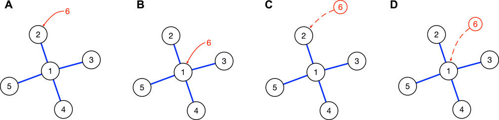
FIGURE 5. The four scenarios in which a non-native species/community can be introduced to a star network: (A) periphery invasion, in which population 6 is introduced directly to niche 2 occupied by population 2; (B) core invasion, in which population 6 is introduced directly to niche 1 occupied by population 1; (C) peripheral niche attachment, in which the niche created by population 6 is attached to niche 2 occupied by population 2; and (D) core niche attachment, in which the niche created by population 6 is attached to niche 1 occupied by population 1. Scenarios (A) and (B) apply to both biological invasion and human migration, whereas scenarios (C) and (D) apply only to human migration, because they involve de novo niche creation.

For scenario (a): periphery invasion, let us assume without loss of generality that the node $i=2$ is attacked. The model defined by Equations (9) and (10) must be modified, so that

$\frac{d{K}_1}{dt}=N_1\left(t\right)\left[{\gamma }_{12}{K}_2\left(t\right)+{\gamma }_{13}{K}_3\left(t\right)+{\gamma }_{14}{K}_4\left(t\right)+{\gamma }_{15}{K}_5\left(t\right)\right]-K_1\left(t\right)\left\{{\gamma }_{21}\left[N_2\left(t\right)+ϵN_6\left(t\right)\right]+{\gamma }_{31}{N}_3\left(t\right)+{\gamma }_{41}{N}_4\left(t\right)+{\gamma }_{51}{N}_5\left(t\right)\right\},$

$\frac{d{K}_2}{dt}={{\gamma }_{21}[N}_2\left(t\right)+ϵN_6\left(t\right)]K_1\left(t\right)-{\gamma }_{12}{K}_2\left(t\right)N_1\left(t\right);$

$\frac{d{N}_2}{dt}={\mu }_2{N}_2\left(t\right)\left[1-\frac{N_2\left(t\right)+N_6\left(t\right)}{K_2\left(t\right)}\right],$

$\frac{d{N}_6}{dt}={\mu }_6{N}_6\left(t\right)\left[1-\frac{N_2\left(t\right)+N_6\left(t\right)}{K_2\left(t\right)}\right].$

In the above equations, the effect of introducing species 6 into node 2 is to increase its effective population, from $N_2\left(t\right)$ to $N_2\left(t\right)+ϵN_6\left(t\right)$. Here, $ϵ$ is a phenomenological parameter that controls how much better species 6 is at exploiting a neighboring niche than species 2 is. If $ϵ<1$, the introduced species ‘steals’ less of the neighboring niche per individual than the native species, to add to the niche it is in. If $ϵ>1$, the introduced species ‘steals’ more of the neighboring niche per individual than the native species, to add to the niche it is in. If $ϵ=1$, which is a special case, the introduced species is just as effective as the native species at exploiting the neighboring niche. Consequently, $ϵ$ does not enter the equations controlling how the populations change. Here, let us note that $ϵ$ can take value greater than 1, because the invasive species can be more aggressive than any of the native species.

On the other hand, for scenario (b): core invasion, we must instead have

$\frac{d{K}_1}{dt}=\left[N_1\left(t\right)+ϵN_6\left(t\right)\right]\left[{\gamma }_{12}{K}_2\left(t\right)+{\gamma }_{13}{K}_3\left(t\right)+{\gamma }_{14}{K}_4\left(t\right)+{\gamma }_{15}{K}_5\left(t\right)\right]-K_1\left(t\right)\left[{\gamma }_{21}{N}_2\left(t\right)+{\gamma }_{31}{N}_3\left(t\right)+{\gamma }_{41}{N}_4\left(t\right)+{\gamma }_{51}{N}_5\left(t\right)\right],$

$\frac{d{K}_i}{dt}=N_i\left(t\right)\left[{\gamma }_{i1}{K}_1\left(t\right)+{\gamma }_{i3}{K}_3\left(t\right)+{\gamma }_{i4}{K}_4\left(t\right)+{\gamma }_{i5}{K}_5\left(t\right)\right]-K_i\left(t\right)\left\{{\gamma }_{1i}\left[N_1\left(t\right)+ϵN_6\left(t\right)\right]+{\gamma }_{3i}{N}_3\left(t\right)+{\gamma }_{4i}{N}_4\left(t\right)+{\gamma }_{5i}{N}_5\left(t\right)\right\},i=2,\dots ,5;$

$\frac{d{N}_1}{dt}={\mu }_1{N}_1\left(t\right)\left[1-\frac{N_1\left(t\right)+N_6\left(t\right)}{K_1\left(t\right)}\right],$

$\frac{d{N}_6}{dt}={\mu }_6{N}_6\left(t\right)\left[1-\frac{N_1\left(t\right)+N_6\left(t\right)}{K_1\left(t\right)}\right].$

After modifying Eqs. 9 and 10 for scenarios (a) and (b), which apply to both biological invasion and human migration, we consider scenarios (c) and (d), which apply only to human migration. Here, let us clarify that in this human migration context, the populations $N_i$ have the usual interpretations, while the carrying capacities $K_i$ are phenomenological quantities that co-evolve with $N_i$ to determine how large these populations will become at equilibrium. In scenarios (c) and (d), the introduced community $N_6$ comes along with its own niche $K_6$. The difference between them is therefore whether niche 6 attaches itself to niche 2 (scenario (c), peripheral attachment), or to niche 1 (scenario (d), core attachment). For the former, we modify the equation governing the change of niche 2,

$\frac{d{K}_2}{dt}=N_2\left(t\right)\left[{\gamma }_{21}{K}_1\left(t\right)+{\gamma }_{26}{K}_6\left(t\right)\right]-K_2\left(t\right)\left[{\gamma }_{12}{N}_1\left(t\right)+{\gamma }_{62}{N}_6\left(t\right)\right],$

and add an equation governing the change of niche 6,

$\frac{d{K}_6}{dt}={\gamma }_{62}{N}_6\left(t\right)K_2\left(t\right)-{\gamma }_{26}{N}_2\left(t\right)K_6\left(t\right).$

We also add one equation governing the change of population of the introduced species 6,

$\frac{d{N}_6}{dt}={\mu }_6{N}_6\left[1-\frac{N_6\left(t\right)}{K_6\left(t\right)}\right].$

The other sub-equations in Equations (9) and (10) remain unchanged.

Finally, for scenario (d), we modify the equation governing the change of niche 1,

$\frac{d{K}_1}{dt}=N_1\left(t\right)\left[{\gamma }_{12}{K}_2\left(t\right)+{\gamma }_{13}{K}_3\left(t\right)+{\gamma }_{14}{K}_4\left(t\right)+{\gamma }_{15}{K}_5\left(t\right)+{\gamma }_{16}{K}_6\left(t\right)\right]-K_1\left(t\right)\left\{{\gamma }_{21}{N}_2\left(t\right)+{\gamma }_{31}{N}_3\left(t\right)+{\gamma }_{41}{N}_4\left(t\right)+{\gamma }_{51}{N}_5\left(t\right)+{\gamma }_{61}{N}_6\left(t\right)\right\},$

add an equation governing the change of niche 6,

$\frac{d{K}_6}{dt}={\gamma }_{61}{N}_6\left(t\right)K_1\left(t\right)-{\gamma }_{16}{N}_1\left(t\right)K_6\left(t\right),$

as well as an equation governing the change of population of the introduced species 6,

$\frac{d{N}_6}{dt}={\mu }_6{N}_6\left[1-\frac{N_6\left(t\right)}{K_6\left(t\right)}\right].$

The other sub-equations in Eqs. 9 and 10 remain unchanged.

4 Simulation results

In this paper, we will focus on what happens on a star network. For simplicity, we assume that ${\mu }_i=0.1$ for all peripheral nodes $i$, but allow the core node 1 to have a larger effective growth rate per capita ${\mu }_1=20$. We also assume ${\gamma }_{ij}=0.02$ for links on the star network, so that all native species/communities are equally competitive. Finally, we introduce some heterogeneity in the simulations by setting the initial carrying capacities to $K_1\left(t=0\right)=1$, $K_i\left(t=0\right)=10$, $i=2,..,5$, and the initial populations to $N_1\left(t=0\right)=1$, $N_2\left(t=0\right)=N_3\left(t=0\right)=N_4\left(t=0\right)=3$, $N_5\left(t=0\right)=1$. We then solve the coupled system of ordinary differential equations for the different scenarios using the function $\mathsf{o}\mathsf{d}\mathsf{e}\mathsf{4}\mathsf{5}\mathsf{(}\mathsf{)}$ in MATLAB. We do this in two stages: (1) from $t=0$ to $t=100$ for $K_i\left(t\right)$ and $N_i\left(t\right)$ to evolve to their equilibrium values, before (2) simulating the invasion from $t=100$ to $t=1000$. Finally, we measure the new equilibrium values $K_i^{*}=\underset{t\to \infty }{\mathit{lim}}{K}_i\left(t\right)$ and $N_i^{*}=\underset{t\to \infty }{\mathit{lim}}{N}_i\left(t\right)$.

4.1 Periphery invasion

When an initial population $N_6\left(0\right)$ of species 6 invades the periphery niche $K_2\left(0\right)$ of species 2, we found from our simulations three different types of equilibria post-invasion: (1) the invasion fails ($N_6^{*}=0$); (2) the invasion succeeds ($N_6^{*}>0$), and there is a partial collapse in the ecosystem; and (3) the invasion succeeds ($N_6^{*}>0$) and all other species remain alive. In the first situation, which occurs when $ϵ<1$ and for all initial populations $N_6\left(0\right)$ as far as we can tell, $K_2^{*}=0$ if ${\mu }_6\le {\mu }_2$, and species 2 also dies ($N_2^{*}=0$) (see Figures 6A,B). This is slightly surprising, as we did not expect $N_2$ to also collapse. On the other hand, if ${\mu }_6>{\mu }_2$, $K_2$ decreases to a new equilibrium value, and species 2 remains alive ($N_2^{*}>0$) (see Figures 6C,D). The carrying capacity lost by node 2 is absorbed by node 1 (the core). We find this last result unintuitive, because according to the standard Lotka-Volterra equation, the species with the larger reproduction rate $\mu$ should survive, but our simulations showed otherwise. In this first situation, the biodiversity decreases slightly.

FIGURE 6

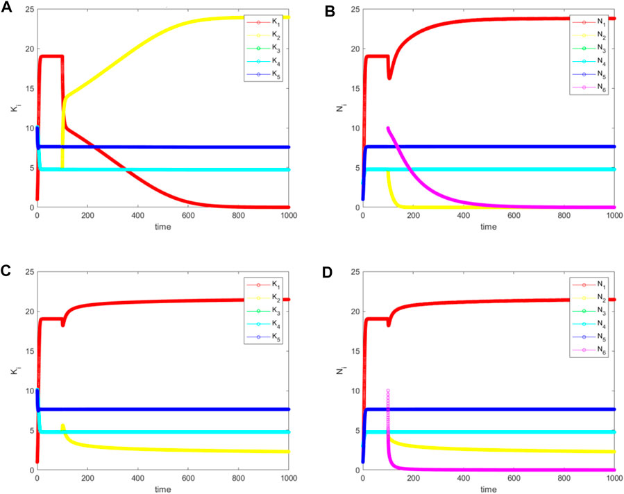
FIGURE 6. The simulated values (A) and (C) for ${\mathit{K}}_i$ and (B) and (D) for $N_i,$ for $ϵ=0.5,{\mu }_6=0.01<{\mu }_2=0.1,N_6\left(0\right)=10,$ and $ϵ=0.5,{\mu }_6=1>{\mu }_2=0.1,N_6\left(0\right)=10,$ respectively. For the simulation shown in (A) and (B), the biodiversity changes from $S_i=0.60$ to $S_f=0.44$, whereas for the simulation shown in (C) and (D), the biodiversity changes from $S_i=0.71$ to $S_f=0.54$.

The second situation occurs when $ϵ\gtrsim 1$, where species 1 (the core) dies (even when ${\mu }_1=20$), whether ${\mu }_6\le {\mu }_2<{\mu }_1$ or ${\mu }_2<{\mu }_6<{\mu }_1$, whatever $N_6\left(0\right)$ is. For ${\mu }_6\le {\mu }_2<{\mu }_1$, we have $N_2^{*}>N_6^{*}$ (Figures 7A,B, in agreement with the reproductive advantage ${\mu }_2>{\mu }_6$), whereas for ${\mu }_2<{\mu }_6<{\mu }_1$, we have $N_6^{*}>N_2^{*}$ (Figures 7C,D, again in agreement with the reproductive advantage ${\mu }_6>{\mu }_2$). In the standard Lotka-Volterra model, co-existence is possible only in the exceptional case when $1-\frac{N_2^{*}+N_6^{*}}{K_2}=0$. In our model, $K_2\left(t\right)$ can evolve with time, and in this second situation, it reaches the equilibrium value associated with $1-\frac{N_2^{*}+N_6^{*}}{K_2^{*}}=0$, whenever $ϵ\gtrsim 1$. This explains why species 2 and 6 can co-exist. In this scenario, full ecological collapse is averted by the fragmentation of the ecosystem ($K_1^{*}=0$). In this second situation, the biodiversity also decreases slightly.

FIGURE 7

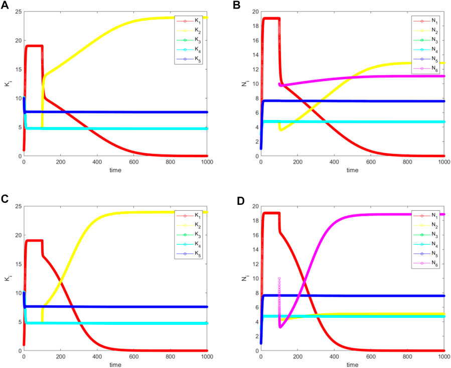
FIGURE 7. The simulated (A) and (C) for ${\mathit{K}}_i$ and (B) and (D) for $N_i$ for $ϵ=1.07,{\mu }_6=0.01<{\mu }_2=0.1,N_6\left(0\right)=10$, and $ϵ=1.05,{\mu }_6=1>{\mu }_2=0.1,N_6\left(0\right)=10$, respectively. For the simulation shown in (A) and (B), the biodiversity changes from $S_i=0.71$ to $S_f=0.67$, whereas for the simulation shown in (C) and (D), the biodiversity changes from $S_i=0.70$ to $S_f=0.62$.

Finally, we find the third situation, which occurs for $ϵ=1$. In this situation shown in Figure 8, the invasion is successful, and species 6 establishes itself, at the expense of species 1 (core) and species 2 (periphery node invaded), but all species are alive. For ${\mu }_6<{\mu }_2$, we end up with $N_6^{*}>N_2^{*}$ if $N_6\left(0\right)\ge N_2\left(0\right)$, but $N_6^{*}<N_2^{*}$ if $N_6\left(0\right)<N_2\left(0\right)$. On the other hand, for ${\mu }_6>{\mu }_2$, we have $N_2^{*}>N_6^{*}$ whatever value $N_6\left(0\right)$ takes. In either case, $K_2$ increases to a new equilibrium value, and its increase is at the expense of node 1 (core). In this third situation, we find either the biodiversity remaining more or less constant, or increasing slightly.

FIGURE 8

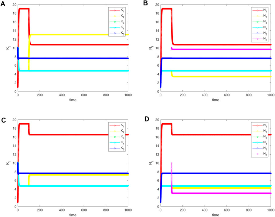
FIGURE 8. The simulated (A) and (C) for $K_i$, and (B) and (D) for $N_i$ for $ϵ=1,{\mu }_6=0.01<{\mu }_2=0.1,N_6\left(0\right)=10$, and $ϵ=1,{\mu }_6=1>{\mu }_2=0.1,N_6\left(0\right)=10$, respectively. For the simulation shown in (A) and (B), the biodiversity changes from $S_i=0.69$ to $S_f=0.73$, whereas for the simulation shown in (C) and (D), the biodiversity changes from $S_i=0.70$ to $S_f=0.69$.

In view of our discussions earlier in this paper, this is the best-case scenario for biological invasion because the biodiversity is slightly increased. However, it only occurs for $ϵ=1$, which is related to the special case of the Lotka-Volterra equation where $K_2^{*}=N_2^{*}+N_6^{*}$, allowing the old species 2 and the new species 6 to coexist on niche $K_2$. However, this scenario remains special, because it requires the invasive species 6 to be identical in exploration efficiency as species 2.

4.2 Core invasion

When species 6 invades the core (species 1), the situation becomes more complex for ${\mu }_6\le {\mu }_1$. There are four distinct regimes: (1) for $ϵ=0.3$, $K_1^{*}>0$, $K_2^{*}=K_3^{*}=K_4^{*}=K_5^{*}=0$, $N_1^{*}>N_6^{*}>0$, $N_2^{*}=N_3^{*}=N_4^{*}=N_5^{*}=0$ (independent of $N_6\left(0\right)$) (near complete ecological collapse, see Figures 9A,B); (2) for $0.4<ϵ<0.6$, we have $N_6^{*}>0$, $N_1^{*}=N_2^{*}=N_3^{*}=N_4^{*}=N_5^{*}=0$ for larger $N_6\left(0\right)$, but $N_1^{*}>0$ also for smaller $N_6\left(0\right)$ (see Figures 9C–F); (3) for $ϵ>0.73$, $K_1^{*}>0$, $K_2^{*}=K_3^{*}=K_4^{*}=K_5^{*}=0$, $N_6^{*}>0$, $N_1^{*}=N_2^{*}=N_3^{*}=N_4^{*}=N_5^{*}=0$ (complete ecological collapse, independent of $N_6\left(0\right)$, see Figures 9G,H). To summarize, for ${\mu }_6<{\mu }_1$, we end up either with $N_1^{*}>N_6^{*}>0$ (near complete ecological collapse) or $N_6^{*}>N_1^{*}=0$ (complete ecological collapse). For smaller ${\mu }_6$, this transition occurs at smaller value of $ϵ$ (between 0.3 and 0.4 for ${\mu }_6=0.01$, and between 0.6 and 0.9 for ${\mu }_6=1$). For ${\mu }_6<{\mu }_1$, there is (4) an additional nonlinear oscillation regime between the two equilibrium phases (see Figures 9I,J, and Section 6 in the Supplementary Material for their phase portraits). This last scenario corresponds to all species co-existing, and therefore biodiversity can potentially increase.

FIGURE 9

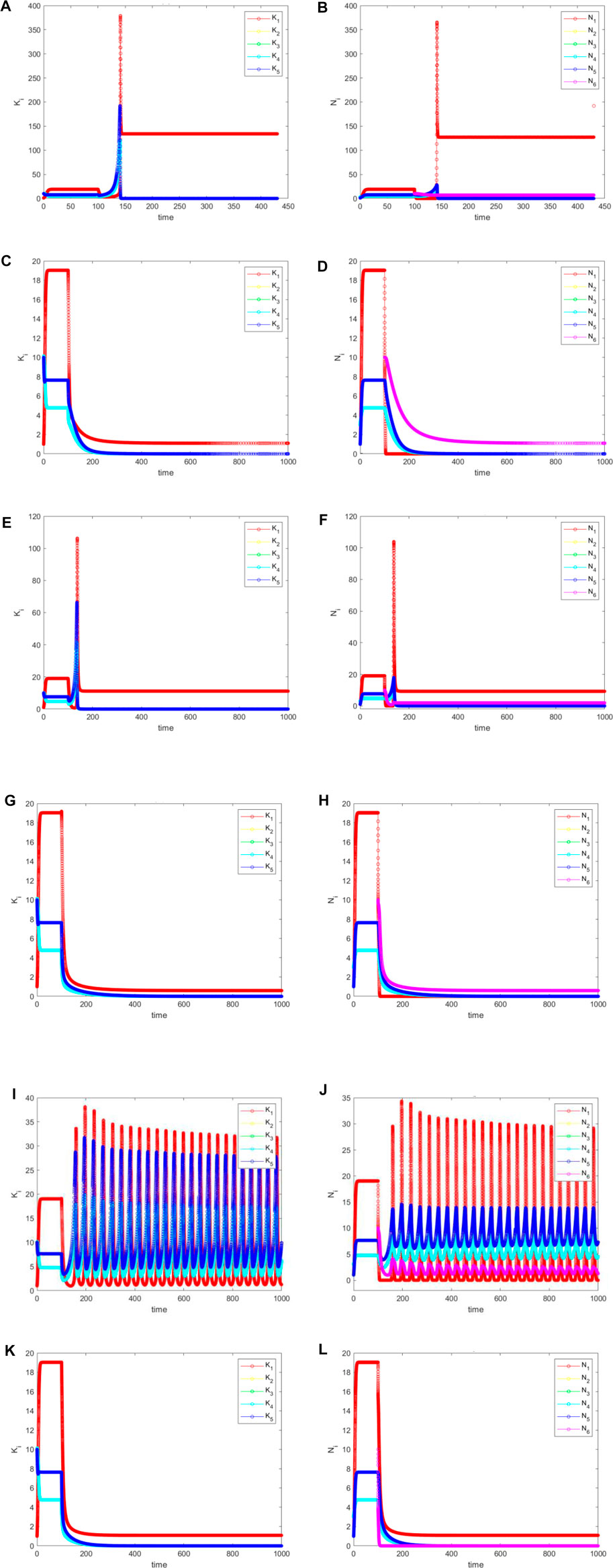
FIGURE 9. (Continued).

For ${\mu }_6>{\mu }_1$, the invasion fails with $N_1^{*}>N_6^{*}=0$ (complete ecological collapse) independent of $N_6\left(0\right)$ (see Figures 9K,L)). We found no signs of nonlinear oscillations whatever $ϵ$ is. We suspect that ecologists may not be aware of this possibility, where the invasion fails, but the ecosystem collapses nonetheless. If we compare this ${\mu }_6>{\mu }_1$ core invasion to the ${\mu }_6>{\mu }_2$ periphery invasion, we find in the latter the invasion also fails, but the ecosystem fragmented, and thus did not collapse. This system of non-overlapping niches is what May foresaw can be accomplished slowly through gradual competition, but it seems like it can also be accomplished rapidly through a failed periphery invasion.

4.3 Niche creation and expansion

4.3.1 Peripheral attachment

Here, the major conclusion is as follows. All populations on the network remain alive, but ${\mathit{K}}_i$ and $N_i$ attain new equilibrium values determined by the initial conditions $N_6\left(0\right)$ and $K_6\left(0\right)$. In particular, we ran simulations with three different values of $N_6\left(0\right)=2,5,10$. Because $K_6$ is connected to $K_2$, ${\mathit{K}}_2^{*}$ and $N_2^{*}$ were directly affected, and $N_1^{*}$, ${\mathit{K}}_1^{*}$ indirectly via species 2. In general, the introduction of $N_6$, ${\mathit{K}}_6$ will reduce $N_1$, ${\mathit{K}}_1$, and $N_2$, ${\mathit{K}}_2$, by values that are determined by $N_6\left(0\right)$ and $K_6\left(0\right)$.

From Figure 10, we see that the population diversity has remained more or less constant after the niche attachment. However, depending on the value added by the new niche, and the values offered by the old niches, if we measure GDP instead this might increase or decrease, depending on the new equilibrium. This overall qualitative conclusion remains the same whatever ${\mu }_6$ is, since ${\mu }_6$ merely controls the relaxation time.

FIGURE 10

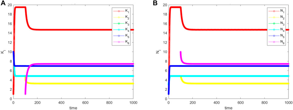
FIGURE 10. The simulated (A) for ${\mathit{K}}_i$ and (B) for $N_i$ for ${\mu }_6=0.01<{\mu }_2=0.1,N_6\left(0\right)=10$. For this simulation, the biodiversity changes from $S_i=0.71$ to $S_f=0.69$.

4.3.2 Core attachment

From Figure 11, we see that $K_1^{*}$ and $N_1^{*}$ decrease because the newly-created $K_6$ is attached to $K_1$. The equilibrium peripheral niches $K_i^{*}$ and populations $N_i^{*}$ for $i=2,3,4,5$ remain unchanged. Comparing this to the case of niche creation and connection to the periphery, we found that when the new niche is connected to the core, only the new niche and the core are affected, whereas when the new niche is connected to the periphery, the new niche, the core, and the periphery node are affected. Interestingly, biodiversity increases when ${\mu }_6$ is smaller than the reproductive rates of the peripheral nodes, and decreases slightly otherwise.

FIGURE 11

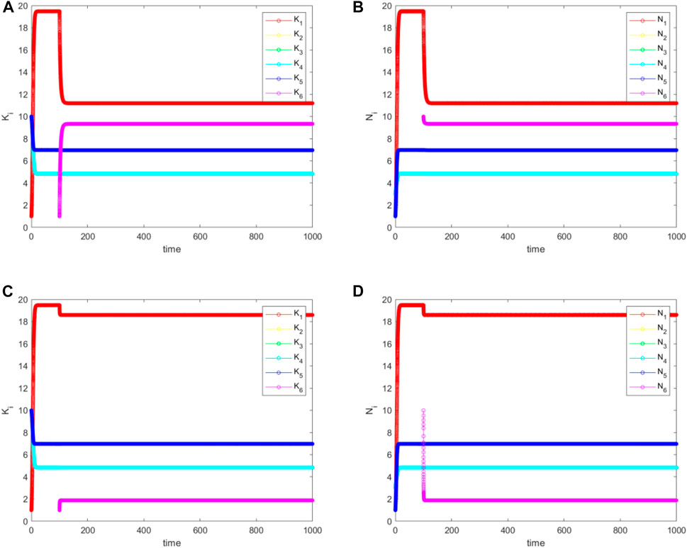
FIGURE 11. The simulated (A), and (C) for ${\mathit{K}}_i$ and (B), and (D) for $N_i$ for $N_6\left(0\right)=10,{\mu }_6=0.01<{\mu }_2=0.1<{\mu }_1=20$, and, $N_6\left(0\right)=10,{\mu }_2=0.1<{\mu }_6=1<{\mu }_1=20$, respectively. For the simulation shown in (A) and (B), the biodiversity changes from $S_i=0.66$ to $S_f=0.71$, whereas for the simulation shown in (C) and (D), the biodiversity changes from $S_i=0.66$ to $S_f=0.62$.

In summary, with niche creation followed by attachment, all populations can survive. If the new niche is connected to a periphery niche, then the populations of this niche and the core niche drops. If the new niche is connected to the core, then there would be no drop in the periphery population, but the core population would drop instead.

5 Discussion

In the simulation results reported in Section 4, we found many surprises. Firstly, we found that the introduction of a non-native species/community into the periphery of an ecosystem/society is not always successful, and not particularly disastrous even when it is successful. Secondly, we found that the introduction of a non-native species/community directly into the core of an ecosystem/society is always catastrophic, whether the non-native species survive in the end. On the other hand, if the non-native species/community creates its own niche when it is introduced, which is possible for human migration but not biological invasion, the outcome is almost always one with equal or higher diversity. These results force us to think more deeply about human migration and biological invasion, as well as the connection between the two, but it would be premature to imagine that we can start developing policies based on these results.

For one, real-world ecosystems are clearly more complex than the star network studied in this paper. To begin with, they have cores that comprise more than one niche. It is also possible to have more than one (and different numbers of) peripheral nodes linked to core nodes. While we expect the effects of peripheral invasion or peripheral niche attachment in real-world ecosystems to be qualitatively similar to what we see for the star network, do we know whether there would be different outcomes for invasion or niche attachment to a core with more than one node? We tested these on the complete network shown in Figure 4A, and found that the ecosystem collapses partially when a non-native species is introduced to one of the nodes. Similar to the star network, the only niche alive after the invasion is the one that is invaded. On the other hand, if the niche created by a non-native species is added to the complete network, all species remain alive, and biodiversity increases.

In this paper, we also allowed only invasions of existing niches (core or peripheral) or niche creations and attachments. Simulations then showed that niche destruction can occur (i.e., $K_i^{*}=0$) because of niche-niche interactions. However, in real-world ecosystems, we may have to consider niches that are destroyed for other reasons (for example, human intervention, which is an extreme form of niche-niche interaction). We have also not considered niche fusion (where two or more niches merge into one as a result of niche-niche interactions). We have also not considered niche fission (where one niche breaks up into two or more niches), which may be important to the discussion of biological invasion or human migration. To put it simply, an initially homogeneous population may become heterogeneous over time, and the sub-populations overlap less and less, to the point where they are better described as homogeneous populations over smaller niches. Specifically, it may also be possible during the invasion that the native population and the introduced population start to develop differences in how they exploit the common niche, leading to this niche fragmenting into two smaller niches. We plan to explore these in future works.

Finally, in the models developed and studied in this paper, we assumed that resources are spatially distributed, but have no independent dynamics of their own. This is clearly an over-simplification, as in real-world ecosystems, resources are sometimes populations, i.e., we have predator populations feeding off prey populations, and privileged human communities exploiting vulnerable human communities. To model these processes, we need more sophisticated models that incorporate trophic levels. In other words, our model can be regarded as the template for one trophic level and must be replicated for other trophic levels. Ultimately, realistic models with multiple resources would be represented on multilayer networks, with one layer for each trophic level of resources. We also need to properly interpret what mutualistic interactions mean in such models and add them whenever necessary.

Besides limitations in our models, we have in this paper only measured the diversities before and after the invasion, in terms of the entropy

$S=-{\displaystyle \sum _{i=1}^S}{p}_i\ln \left(p_i\right),p_i=\frac{N_i}{N_1+N_2+\dots +N_S}.$

However, one might argue that diversity is not the most important decision-making criterion, even though it is frequently invoked. For human migration (and to some extent also the introduction of non-native biological species), economic reasons are more important.

Within the framework of our models, there are two main sources of economic contributions: (1) within niches (representing the economic interactions between members of the same niches), and (2) between niches (representing economic interactions between members of different niches). These economic interactions are clear for human migration but less so for the introduction of non-native biological species. Let us take the opportunity to clarify: the economic value of an ecosystem is to us, the human society. Therefore, we are the ones who assign values to different parts of an ecosystem. For example, if we are of the opinion that the ecosystem services provided by bees are important to us, but not those provided by ants or cockroaches, we can assign a positive economic value to bees, but zero (or even negative) economic value to ants and cockroaches. We can then sum over different parts of the ecosystem to determine its net economic value. From this point of view, we would only bring in a non-native biological species that we consider economically valuable. However, we would also like to gauge the effects of the introduction of this non-native biological species have on the whole ecosystem, by waiting for the ecosystem to reach its new equilibrium, and thereafter computing the net economic value. If the net economic value is increased (because the introduction leads to decreases in the populations of ants and cockroaches), we can proceed with the introduction. Else, if the net economic value is decreased (because the population of bees is decreased, or the populations of ants and cockroaches are increased), we do not go ahead with the introduction.

Finally, for human migration, we need to consider what the niches actually represent, i.e., do they represent different employment sectors, or can they be different combinations of employment sectors? Indeed, a non-native population settling down in society by offering unique products and services reminds us of Type 3 human migration under McNeil’s classification scheme. In the past, these migrants can settle down at the edge of towns and villages, and therefore constitute minimal competition to existing communities. Today, migrants arriving in urban settlements must necessarily compete with existing communities, even if they come with unique skills or are willing to take on undesirable jobs. For example, when East Asian migrants arrive in a new city, they frequently create a Chinatown or Koreatown or Vietnamtown, because the establishment of the niche pulls in more migrants from the same region. Once established, the niche displaces whatever was there in the first place, but its economic trajectory is not yet certain. In some cases, the niche becomes a slum, with low employment, high crime, low economic productivity, and generally a menace to the other niches it borders. In other cases, the niche can become attractions, as many Chinatowns do with their offerings of affordable Chinese restaurants and Chinese supermarkets. Naturally, these proliferated initially to serve the migrant population, but later expanded because they are also liked by locals, thereby adding economic value to neighbouring niches.

As mentioned, we would like the models we developed in this paper to help facilitate ethical discussions on domestic and international migration. Nevertheless, we believe that these are not final answers, but only the beginning of scientific debates. For example, a seemingly important question that any immigration policy is forced to address is how many migrants a society can accommodate. We find from our simulations that this is not really the correct question to ask, since the qualitative outcomes seem to not depend on the initial number of introduced individuals. On the other hand, the quality of these immigrants seemed to be far more important, whether they come in via periphery invasion, core invasion, niche creation followed by peripheral attachment, or niche creation followed by core attachment. Negative consequences (sometimes catastrophic) seem to be possible, if immigrants who are more hardworking and less picky about jobs are directly inserted into populated niches to compete against less hardworking and more picky natives. The general recommendation from our simulation results seems to be: if the immigrants are highly skilled (with expertise absent in natives), they come with their own niche, which can be attached to any existing niches. If the immigrants are unskilled, they should be guided to an unpopulated niche, so that they do not compete directly with the natives.

6 Conclusion

In conclusion, we synthesized three disparate literatures on (1) human migration, (2) biological invasion, both in recent times where records were available, with that on archaeological studies on human migration and dispersal of non-native plants and animals, to argue that the popular views that human migration is good but biological invasion is bad represent a paradoxical and incomplete view on the two highly similar phenomena. We then proposed to resolve this apparent paradox through modelling and simulations. To do this, we reviewed the definitions and literatures on niches in ecology, culture, technology and innovation, before developing our own operational definition of niches that accommodates niche-niche interactions. Thereafter, we wrote down sets of ordinary differential equation models of these interactions on a star network, for isolated ecosystems or communities, as well as those experiencing invasions (or niche attachments) at a periphery node or the core node.

For invasions, whereby a non-native population is introduced directly into the niche of a native population, we found three different types of equilibria post-invasion if the invasion occurs at the periphery of the network. In the first case, where the non-native population is less effective in exploring neighbouring niches than the native population it is invading, the invasion fails however large the initial invading population. The native population being invaded can sometimes also perish, but remain alive in other times. In the remaining two cases, where the invasion is successful, we can have either all species remaining alive, or a partial ecological collapse. When the non-native population invades the core niche, on the other hand, we almost always end up with a complete or near complete ecological collapse. In contrast, when the non-native population creates a niche of its own (or occupy an existing but vacant niche) that subsequently attaches itself to the community (we do not believe that such processes are possible in ecosystems), all populations survive and the cultural diversity after niche attachment is sometimes higher than before.

We believe that the models and simulation results reported in this paper offer new insights and theoretical grounds for policymakers to start ethical discussions of immigration issues on firm scientific foundations. In particular, our simulations showed that diversity can be increased through the introduction of non-native populations, without exacting a heavy price from the native populations. Because of the simple interpretations of the processes introduced, our results can be easily translated into immigration policies that are kinder towards the natives as well as the immigrants. However, we are mindful that we have only analysed outcomes in a toy model of ecosystems or communities. More studies with realistic network models, including those with multiple trophic levels, will be necessary to see how universal our results are. Further studies measuring performance metrics other than diversity are also welcome.

Data availability statement

The MATLAB scripts used in this study can be found in https://doi.org/10.21979/N9/LQX1MS.

Author contributions

SC conceived the study, SC and PT-WY wrote the code and simulated the data, SC and PT-WY analysed the data and interpreted the results, SC and PT-WY wrote and reviewed the manuscript. All authors contributed to the article and approved the submitted version.

Conflict of interest

The authors declare that the research was conducted in the absence of any commercial or financial relationships that could be construed as a potential conflict of interest.

Publisher’s note

All claims expressed in this article are solely those of the authors and do not necessarily represent those of their affiliated organizations, or those of the publisher, the editors and the reviewers. Any product that may be evaluated in this article, or claim that may be made by its manufacturer, is not guaranteed or endorsed by the publisher.

Supplementary material

The Supplementary Material for this article can be found online at: https://www.frontiersin.org/articles/10.3389/fphy.2023.1088699/full#supplementary-material

References

1.UNHCR. Ukraine refugee situation: Operation data portal (2022). Available at: https://data.unhcr.org/en/situations/ukraine.

Google Scholar

2. Connor P. Most displaced Syrians are in the Middle East, and about a million are in europe: Pew research center (2018). Available at: https://www.pewresearch.org/fact-tank/2018/01/29/where-displaced-syrians-have-resettled/.

Google Scholar

3.UNHCR Uf. Syria refugee crisis explained (2022). Available at: https://www.unrefugees.org/news/syria-refugee-crisis-explained/.

Google Scholar

4. Sullivan EAJ. Miriam. Illegal border crossings, driven by pandemic and natural disasters (2021). Available at: https://www.nytimes.com/2021/10/22/us/politics/border-crossings-immigration-record-high.html.

Google Scholar

5. Pérez S, Michelle H. Record numbers of migrants arrested at southern border, with two million annual total in sight (2022). Available at: https://www.wsj.com/articles/illegal-immigration-arrests-hit-record-reasons-for-border-crossings-changing-11660599304.

Google Scholar

6.M McAuliffe, and B Khadria, editors. World migration report 2020 (2019).

Google Scholar

7.TIOf Migration. Global compact for migration (2022). Available at: https://www.iom.int/global-compact-migration.

Google Scholar

8. Sherman A, Trisi D, Stone C, Gonzales S, Parrott S. Immigrants contribute greatly to US economy, despite administration’s “public charge” rule rationale. Washington DC: Center on Budget and Policy Priorities (CBPP) (2019). Available at: https://www.cbpp.org/research/poverty-and-inequality/immigrants-contribute-greatly-to-us-economy-despite-administrations.

Google Scholar

9. Sirkeci I, Cohen JH, Přívara A. Towards a migration letters index: The most influential works and authors in migration studies. Migration Lett (2017) 14(3):397–424. doi:10.33182/ml.v14i3.352

CrossRef Full Text | Google Scholar

10. Ravenstein EG. The laws of migration. J Stat Soc Lond (1885) 48(2):167–235. doi:10.2307/2979181

CrossRef Full Text | Google Scholar

11. Ravenstein EG. The laws of migration. J R Stat Soc (1889) 52(2):241–305. doi:10.2307/2979333

CrossRef Full Text | Google Scholar

12. Thomas WI, Znaniecki F. The Polish peasant in Europe and America: Monograph of an immigrant group. Chicago, IL: University of Chicago Press (1919).

Google Scholar

13. Jean-Christophe Dumont TL. Is migration good for the economy? Paris, France: OECD Migration Policy Debates (2014). Available at: https://www.oecd.org/migration/OECD%20Migration%20Policy%20Debates%20Numero%202.pdf.

Google Scholar

14. Goldin I. How immigration has changed the world—for the better (2016). Available at: https://www.weforum.org/agenda/2016/01/how-immigration-has-changed-the-world-for-the-better/.

15. Fang T. The immigration jump: Are more immigrants good for the economy? (2016). Available at: https://wol.iza.org/opinions/the-immigration-jump-are-more-immigrants-good-for-the-economy.

Google Scholar

16. Nowrasteh A. The 14 most common arguments against immigration and why they’re wrong (2018). Available at: https://www.cato.org/blog/14-most-common-arguments-against-immigration-why-theyre-wrong.

Google Scholar

17. Beck RH. The case against immigration: The moral, economic, social, and environmental reasons for reducing US immigration back to traditional levels. New York, NY: W. W. Norton & Company (1996).

Google Scholar

18. Williamson M. Biological invasions. London, UK: Chapman & Hall (1996).

Google Scholar

19. Ricklefs RE. Taxon cycles: insights from invasive species. In: DF Sax, JJ Stachowicz, and SD Gaines, editors Species Invasions: Insights into Ecology, Evolution, and Biogeography. Sunderland, MA: Sinauer Associates (2005). p. 165–199.

Google Scholar

20. Reise K, Olenin S, Thieltges DW. Are aliens threatening European aquatic coastal ecosystems? Helgol Mar Res (2006) 60:77–83. doi:10.1007/s10152-006-0024-9

CrossRef Full Text | Google Scholar

21. Henderson S, Dawson TP, Whittaker RJ. Progress in invasive plants research. Prog Phys Geogr (2006) 30(1):25–46. doi:10.1191/0309133306pp468ra

CrossRef Full Text | Google Scholar

22. Pimentel D, Zuniga R, Morrison D. Update on the environmental and economic costs associated with alien-invasive species in the United States. Ecol Econ (2005) 52(3):273–88. doi:10.1016/j.ecolecon.2004.10.002

CrossRef Full Text | Google Scholar

23. Chew MK. Ending with Elton preludes to invasion biology. AZ: Arizona State University Tempe (2006).

Google Scholar

24. Cadotte MW. Darwin to Elton: Early ecology and the problem of invasive species. In: Conceptual ecology and invasion biology: Reciprocal approaches to nature. Dordrecht, Netherlands: Springer (2006). p. 15–33.

Google Scholar

25. Fitch A. Fifth report on the noxious and other insects of the state of New York. Trans New York Agric Soc (1859) 18:781–854.

Google Scholar

26. Forbes SA. The lake as a microcosm. Illinois Natural History Survey Bulletin (1887) 15(1925): 537–550. Reproduced in: LE Keup, WM Ingram, and KM Mackenthun, editors Biology of water pollution: a collection of selected papers on stream pollution, waste water, and water treatment. Washington, DC: US Department of the Interior (1967). p. 3–9.

Google Scholar

27. Forbes SA. The season’s campaign against the San José and other scale insects in Illinois. Trans Ill State Hortic Soc (1898) 31:105–19.

Google Scholar

28. Howard LO. The spread of land species by the agency of Man; with especial reference to insects. Science (1897) 6(141):18160–1. doi:10.1038/scientificamerican10091897-18160supp

CrossRef Full Text | Google Scholar

29. Elton CS. The ecology of invasions by animals and plants, 2nd Edn. Cham, Switzerland: Springer (2020).

Google Scholar

30. Spalding VM. Distribution and movements of desert plants. Washington, DC: Carnegie institution of Washington (1909).

Google Scholar

31. Price TD, Sol D. Introduction: Genetics of colonizing species. The Am Naturalist (2008) 172(S1):S1–S3. doi:10.1086/588639

PubMed Abstract | CrossRef Full Text | Google Scholar

32. Davis MA. Invasion biology. New York, NY: Oxford University Press on Demand (2009).

Google Scholar

33. White TD, Asfaw B, DeGusta D, Gilbert H, Richards GD, Suwa G, et al. Pleistocene homo sapiens from middle awash, Ethiopia. Nature (2003) 423(6941):742–7. doi:10.1038/nature01669

PubMed Abstract | CrossRef Full Text | Google Scholar

34. Posth C, Renaud G, Mittnik A, Drucker DG, Rougier H, Cupillard C, et al. Pleistocene mitochondrial genomes suggest a single major dispersal of non-Africans and a Late Glacial population turnover in Europe. Curr Biol (2016) 26(6):557–61. doi:10.1016/j.cub.2016.02.022

PubMed Abstract | CrossRef Full Text | Google Scholar

35. Haber M, Jones AL, Connell BA, Arciero E, Yang H, Thomas MG, et al. A rare deep-rooting D0 African Y-chromosomal haplogroup and its implications for the expansion of modern humans out of Africa. Genetics (2019) 212(4):1421–8. doi:10.1534/genetics.119.302368

PubMed Abstract | CrossRef Full Text | Google Scholar

36. Flegontov P, Altınışık NE, Changmai P, Rohland N, Mallick S, Adamski N, et al. Palaeo-Eskimo genetic ancestry and the peopling of Chukotka and North America. Nature (2019) 570(7760):236–40. doi:10.1038/s41586-019-1251-y

PubMed Abstract | CrossRef Full Text | Google Scholar

37. McNeill WH. Human migration in historical perspective. Popul Dev Rev (1984) 10:1–18. doi:10.2307/1973159

CrossRef Full Text | Google Scholar

38. Gu S. Language and culture in the growth of imperialism. Jefferson, NC: McFarland (2012).

Google Scholar

39. Kitchen A, Ehret C, Assefa S, Mulligan CJ. Bayesian phylogenetic analysis of semitic languages identifies an early bronze age origin of semitic in the near East. Proc R Soc B: Biol Sci (2009) 276(1668):2703–10. doi:10.1098/rspb.2009.0408

PubMed Abstract | CrossRef Full Text | Google Scholar

40. Phillipson DW. Foundations of an african civilisation: Aksum & the northern horn, 1000 BC-1300 AD. Suffolk, UK: Boydell & Brewer Ltd (2012).

Google Scholar

41. Normile D. Yangtze seen as earliest rice site. Science (1997) 275(5298):309. doi:10.1126/science.275.5298.309

CrossRef Full Text | Google Scholar

42. Ahn S-M. The emergence of rice agriculture in korea: Archaeobotanical perspectives. Archaeological anthropological Sci (2010) 2(2):89–98. doi:10.1007/s12520-010-0029-9

CrossRef Full Text | Google Scholar

43. Nakagahra M, Okuno K, Vaughan D. Rice genetic resources: History, conservation, investigative characterization and use in Japan. In: Sasaki T, Moore G editors, Oryza: From molecule to plant. Dordrecht, Netherlands: Kluwer Academic Publishers (1997). p. 69–77.

PubMed Abstract | CrossRef Full Text | Google Scholar

44. Fuller DQ. An agricultural perspective on dravidian historical linguistics: Archaeological crop packages, livestock and dravidian crop vocabulary In: Renfrew C, Bellwood PS editors, Examining the farming/language dispersal hypothesis. Cambridge, UK: McDonald Institute for Archaeological Research (2003). p. 191–213.

Google Scholar

45. Rosenberg M, Redding RW. Implications for modeling the origins of food production In: Nelson SM, Ancestors for the pigs: pigs in prehistory. Philadelphia, PA: University of Pennsylvania Press (1998). pp. 15–55.

Google Scholar

46. Nelson S. Introduction: pigs in prehistory In: Nelson S, editors, Ancestors for the pigs: pigs in prehistory. Philadelphia, PA: University of Pennsylvania Press (1998). pp. 1–4.

Google Scholar

47. Jing Y, Flad RK. Pig domestication in ancient China. Antiquity (2002) 76(293):724–32. doi:10.1017/s0003598x00091171

CrossRef Full Text | Google Scholar

48. Bosse M. A genomics perspective on pig domestication In: Teletchea F, editors, Animal Domestication. London, UK: IntechOpen (2018).

Google Scholar

49. Arbuckle BS, Kansa SW, Kansa E, Orton D, Çakırlar C, Gourichon L, et al. Data sharing reveals complexity in the westward spread of domestic animals across Neolithic Turkey. PloS one (2014) 9(6):e99845. doi:10.1371/journal.pone.0099845

PubMed Abstract | CrossRef Full Text | Google Scholar

50. Larson G, Albarella U, Dobney K, Rowley-Conwy P, Schibler J, Tresset A, et al. Ancient DNA, pig domestication, and the spread of the Neolithic into Europe. Proc Natl Acad Sci (2007) 104(39):15276–81. doi:10.1073/pnas.0703411104

PubMed Abstract | CrossRef Full Text | Google Scholar

51. Ramos-Onsins SE, Burgos-Paz W, Manunza A, Amills M. Mining the pig genome to investigate the domestication process. Heredity (2014) 113(6):471–84. doi:10.1038/hdy.2014.68

PubMed Abstract | CrossRef Full Text | Google Scholar

52. Cameron TWM. The pig and human disease. Proc Royal Soc Med (1924) 17(9): 31–37.

CrossRef Full Text | Google Scholar

53. Borjas GS. Yes, immigration hurts American workers: Politico (2016). Available at: https://www.politico.com/magazine/story/2016/09/trump-clinton-immigration-economy-unemployment-jobs-214216/.

Google Scholar

54. Borjas GJ. The labor demand curve is downward sloping: Reexamining the impact of immigration on the labor market. Q J Econ (2003) 118(4):1335–74. doi:10.1162/003355303322552810

CrossRef Full Text | Google Scholar

55.IOM. World on the move: The benefits of migration (2014). Available at: https://www.iom.int/speeches-and-talks/world-move-benefits-migration.

Google Scholar

56. May RM. Stability and complexity in model ecosystems. Princeton, NJ: Princeton university press (2019).

Google Scholar

57. Laland KN, Odling-Smee J, Feldman MW. Niche construction, biological evolution, and cultural change. Behav Brain Sci (2000) 23(1):131–46. doi:10.1017/s0140525x00002417

PubMed Abstract | CrossRef Full Text | Google Scholar

58. Jordano P, Bascompte J, Olesen JM. The ecological consequences of complex topology and nested structure in pollination webs. Plant-pollinator interactions: from specialization to generalization (2006) 173–99.

Google Scholar

59. Dobson A. Food-web structure and ecosystem services: Insights from the serengeti. Philos Trans R Soc B: Biol Sci (2009) 364(1524):1665–82. doi:10.1098/rstb.2008.0287

PubMed Abstract | CrossRef Full Text | Google Scholar

60. Kondoh M, Kato S, Sakato Y. Food webs are built up with nested subwebs. Ecology (2010) 91(11):3123–30. doi:10.1890/09-2219.1

PubMed Abstract | CrossRef Full Text | Google Scholar

61. Suweis S, Simini F, Banavar JR, Maritan A. Emergence of structural and dynamical properties of ecological mutualistic networks. Nature (2013) 500(7463):449–52. doi:10.1038/nature12438

PubMed Abstract | CrossRef Full Text | Google Scholar

62. Miele V, Ramos-Jiliberto R, Vázquez DP. Core–periphery dynamics in a plant–pollinator network. J Anim Ecol (2020) 89(7):1670–7. doi:10.1111/1365-2656.13217

PubMed Abstract | CrossRef Full Text | Google Scholar

63. Csermely P, London A, Wu L-Y, Uzzi B. Structure and dynamics of core/periphery networks. J Complex Networks (2013) 1(2):93–123. doi:10.1093/comnet/cnt016

CrossRef Full Text | Google Scholar

64. Lee SH. Network nestedness as generalized core-periphery structures. Phys Rev E (2016) 93(2):022306. doi:10.1103/physreve.93.022306

PubMed Abstract | CrossRef Full Text | Google Scholar

65. Suweis S, Grilli J, Banavar JR, Allesina S, Maritan A. Effect of localization on the stability of mutualistic ecological networks. Nat Commun (2015) 6(1):10179–7. doi:10.1038/ncomms10179

PubMed Abstract | CrossRef Full Text | Google Scholar