Economic cascades, tipping points, and the costs of a business-as-usual approach to COVID-19

Decisions to shutdown economic activities to control the spread of COVID-19 early in the pandemic remain controversial, with negative impacts including high rates of unemployment. Here we present a counterfactual scenario for the state of California in which the economy remained open and active during the pandemic’s first year. The exercise provides a baseline against which to compare actual levels of job losses. We developed an economic-epidemiological mathematical model to simulate outbreaks of COVID-19 in ten large Californian socio-economic areas. Results show that job losses are an unavoidable consequence of the pandemic, because even in an open economy, debilitating illness and death among workers drive economic downturns. Although job losses in the counterfactual scenario were predicted to be less than those actually experienced, the cost would have been the additional death or disablement of tens of thousands of workers. Furthermore, whereas an open economy would have favoured populous, services-oriented coastal areas in terms of employment, the opposite would have been true of smaller inland areas and those with relatively larger agricultural sectors. Thus, in addition to the greater cost in lives, the benefits of maintaining economic activity would have been unequally distributed, exacerbating other realized social inequities of the disease’s impact.

1 Introduction

When the COVID-19 global pandemic emerged in early 2020, there were no preventive vaccines or effective medical treatments available. Following standard epidemiological procedures, initial responses in most affected countries and municipalities focused on disrupting transmission of the disease. Examples of responses included travel bans, the closure of public venues and workplaces, and isolation of infected individuals and sometimes of their communities. The abruptness and rapidity with which so-called shutdown measures proceeded, coupled with the measures themselves, sent a shock wave through the global economy [1, 2]. The ensuing economic hardship added to the health and other social impacts of the disease, and in many countries were vigorously opposed from multiple and diverse economic and political quarters [3]. A common argument in the United States, where the implementation of “economic shutdown” was heterogeneous in both timing and extent, was that economic damage could exceed the potential damage of the disease itself [4].

The situation at the time of this writing, differs with the availability of both effective vaccines, and post-infection treatments. After suffering a tremendous death toll from the disease (more than one million), a major portion ($>$71%) of the American population has received at least two doses of a vaccine (US Centers for Disease Control), and although hospitalization rates oscillate with the emergence of new and highly virulent genetic strains of the virus, mortality rates are significantly lower than during the first year of the pandemic. Furthermore, the steep decline of employment in 2020 has been reversed to a considerable degree—from an unemployment high of 14.7% in April, 2020 to 3.6% in April, 2022 (US Bureau of Labor Statistics). Partial economic shutdowns remain a possibility if the number of infected persons increases, and the question of economic versus human health continues to be asked in response.

The question is a difficult one to answer, because it is impossible to know what the outcome would have been if no shutdown measures were implemented. One could look to other countries where measures differed or varied, but any comparisons are complicated by numerous factors, including political system, socio-economic structure, governmental policies and leadership, demographic structure, healthcare systems, and socio-behavioural norms. The question can be addressed, however, as a counterfactual one, where one examines a situation that did not occur, but that could have occurred [5].

In this paper, we examine a counterfactual situation in which the American state of California did not implement an economic shutdown in 2020, but instead weathered the first wave of the pandemic with an open economy. We develop a network model of dynamic relationships among industrial sectors of several major economic regions within the state, and simulate the impact of an unmitigated outbreak of COVID-19 on the health and employment of the employed labour force at the beginning of March, 2020. Those impacts are estimated by driving the dynamic economic model with an SIR (Susceptible, Infected, Recovered) epidemiological model, parameterized with real disease and demographic data. In so doing, we are able to explore the counterfactual situation of what could have happened, and compare it to real outcomes that resulted from the economic shutdowns.

California presents a suitable case for examination because the state’s economy is comparable in size to those of many nation states’, ranking as the world’s $5^{\mathtt{t}\mathtt{h}}$ largest in 2019 [6]. Yet, socio-economic systems (SESs) within the state, including those used here, span orders of magnitude in size and economic activity–the smallest SES examined, Stockton-Lodi, had a workforce of 258,300 employees in February, 2020, whereas the Los Angeles-Long Beach-Glendale SES’s was 4,636,800. The SESs are also structurally diverse, comprising systems dominated by goods producing versus services providing industries, delineated roughly according to inland or coastal locations. Furthermore, California acted early during the emergence of the pandemic in the United States, declaring a state of emergency on March $4^{\mathtt{t}\mathtt{h}}$ 2020, and statewide shelter-in-place orders, social distancing policies, and the closure of non-essential businesses on March ${19}^{\mathtt{t}\mathtt{h}}$. The economic reaction was severe and nearly immediate, with more than two million workers in our SES set being newly unemployed by April 2020. California’s economy and its regional components may thus serve as suitable analogs for SESs elsewhere.

We applied the model to ten major metropolitan areas, SESs, in California, modeling outbreaks for a range of transmission intensities, including those estimated to have actually occurred within the areas in March, 2020. Our California SESs are metropolitan divisions (MDs) or metropolitan statistical areas (MSAs) delineated by the United States Office of Management and Budget and utilized by the United States Bureau of Labor Statistics (USBLS) and the California Employment and Development Department (CAEDD) for reporting economic data. They include: San Francisco-San Mateo-Redwood City MD, Oakland-Berkeley-Livermore MD, San Jose-Sunnyvale-Santa Clara MSA, Stockton-Lodi MSA, Fresno MSA, Los Angeles-Long Beach-Glendale MD, Anaheim-Santa Ana-Irvine MD, Riverside-San Bernardino-Ontario MSA, Oxnard-Thousand Oaks-Ventura MSA, and San Diego-Carlsbad MSA [7, 8] (Figure 1A).

FIGURE 1

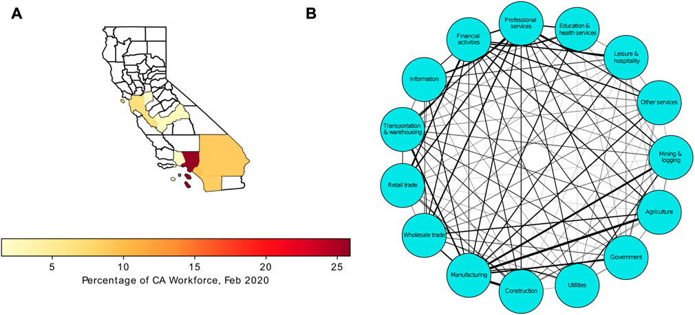
FIGURE 1. (A) California metropolitan areas representative of SESs. Color bar shows the percentage of the total California workforce in February, 2020. (B) The US inter-industry network. Link widths are scaled according to total inter-sector exchange strengths (μ in Eq. 3; see Materials and Methods; Supplementary Dataset S2). Thicker links indicate stronger inter-sector dependencies. Note that “Agriculture” here is equal to employment listed as “Total Farm” by the CAEDD.

The model predicts the loss of employment within an SES driven by mortality and severe illness, as well as losses caused by the subsequent reductions of production and demand within the SES. Finally, we compared model predictions based on the initial contagiousness of an outbreak (R₀) to those that resulted from real-world mitigation efforts and reduced rates of transmission (“flattening the curve;” R-effective, or $R_{\mathtt{e}\mathtt{f}\mathtt{f}}$). The epidemiological-economic model subsequently simulates the number of jobs lost within sectors and SESs under a range of outbreak severities. The model is analogous to, and draws inspiration from, closed mass balance or closed ecosystem models such as those employed in thermodynamics and ecology respectively. SESs are treated as complex networks of interacting industries or sectors, with sectors having mutualistic relationships of supply and demand, similar to the mutualistic interactions among species within ecological communities. We take advantage of the considerable body of work demonstrating the complex responses and emergent properties of such systems to a variety of perturbations [9–12], as well as the conceptual connections between ecological and economic networks as complex systems [13].

2 Materials and methods

2.1 The CASES model

The counterfactual model, which we term the “business-as-usual CASES (Complex Adaptive Socio-Economic Systems) model,” is a compartmental network model that treats employment within an industrial sector as a function of employment levels in all sectors, mediated by the value of inter-industry exchanges. Each SES is represented as a network of industrial sectors linked by the exchange of goods and services between sectors (Figure 1B). The sectors represent the major goods producing and services providing sectors within the North America Industry Classification System as utilized by the USBLS and CAEDD (Supplementary File S1). These particular socio-economic systems were selected primarily because of the availability of monthly employment data for the fifteen major industrial sectors used by the USBLS to aggregate economic activity in the United States during the relevant time interval (February, 2020 to March, 2021). We used seasonally unadjusted data [14, 15], and included the Agriculture industrial sector (Total Farm) both for completeness of the data, and the importance of, albeit relatively smaller, farming components of the SESs. Each sector is an aggregation of related industries; for example, filmmakers, film distributors, and cinemas are all assigned to the Leisure and Hospitality sector. There are economic exchanges both between and within sectors, for example, Leisure and Hospitality requires products from the Manufacturing and Wholesale Trade sectors. The model postulates that the strengths of interactions vary according to the mutualistic dependencies of supply and demand between sectors.

The model also assumes that the number of employed workers in a sector is a function of sufficient supply of necessary materials or services to the sector, and the demand for its products and services. Those supplies and demands are thus also functions of employment levels in all sectors. The inter-dependencies are described with a set of coupled ordinary differential equations (ODEs) (see below). If a model SES is isolated from variations of external input and output variables, such as external subsidies and consumer demand, the system will reach an equilibrium in which employment within sectors remains constant. Our approach is thus to isolate an SES in this manner, and to then introduce a perturbation representing the loss of workers to COVID-19 infection, specifically disabling disease or death. The system of ODEs then measures, over time, the cascading consequences of the outbreak as workers are lost to infection, or jobs are lost because of the impact on inter-sector supply and demand. Such cascades are well recognized and unavoidable consequences of both networked systems (the inter-industry network) and their internal feedback processes (e.g., the partial regulation of sector activity by the activities of other sectors) [16, 17]. The timing, frequency and magnitude of a cascade are often hard or impossible to predict in complex systems on the basis of input data alone, and forecasting can only be done with the analysis or simulation of models that capture the salient features of such systems.

The outbreak and progression of the disease is modelled with an SIR epidemiological model (Supplementary Material). COVID-19 affects individuals differently based on age and pre-existing conditions. We account for age dependencies by modeling the disease dynamics of age classes within sectors, but unfortunately there are insufficient data within sectors regarding exacerbating pre-conditions, either medical or socio-economic (for example, income levels), and how those interact with the disease to affect worker health.

2.2 SES networks

SES networks represent each industrial sector as a node (for example, [18, 19]). Nodes are linked by exchanges of goods and services, and all nodes or sectors interact economically. The inter-sector links are bi-directional, representing the generally asymmetric requirements between sectors. Link weights, which represent the strengths of the interactions between two sectors, are derived from the value of inter-industry exchanges for the United States during 2019 (US Bureau of Economic Analysis; Supplementary File S2), and based ultimately on input-output evaluations [20]. Total sector requirements are normalized, with all sector requirements, including intra-sector trade, summing to 1. Normalization scales all inter-sector interactions relative to each other, rendering them dimensionless and more directly comparable to the total flux of industry exchanges in the system. Furthermore, because the model assumes that an unperturbed system is initially in a static equilibrium, any subsequent deviations from that equilibrium are trivially relative to unity, or one. Link weights are thus calculated as

$w_{ij}=\frac{q_{ij}}{{\sum }_{n=1}^S\left(q_{in}+q_{ni}\right)}(1)$

where q_ij is the industry by industry total requirement, that is, the amount of industry j’s production that is required by industry i. S is the number of sectors. The input-output interactions are the monetary values of the input to sector i from j, and output from i to j. The resulting matrix W comprises the elements w_ij and w_ji (Supplementary File S2), and is asymmetric, as the demands and supplies between sectors are rarely equal.

2.3 Model outline

Employment in sector i is modeled as responding when external drivers remove or add workers, or labour, to the sector. Here we consider negative drivers only, that is, the loss of workers specifically to mortality or long-term debilitating illness. If we represent those drivers collectively as the rate at which a fraction of the employed workforce is removed, and the internal dependence of the sector on its own production, then the rate of change of employment is a function of the magnitude of the removal rate.

Sector employment, however, is also a function of employment in other sectors, per the SES network, and disease-driven reductions in any other sector j therefore leads to further unemployment in i as supply and/or demand decline. Those inter-sectoral interactions, plus intra-sectoral dependencies (Eq. 2) are described as

$\frac{d{E}_i}{dt}=-{\varphi }_i{E}_i\left[w_{ii}+\sum _{j=1}^S\left(w_{ij}\frac{E_j}{E_j\left(0\right)}+w_{ji}\frac{E_j}{E_j\left(0\right)}\right)\right](2)$

where E_i is employment in sector i, ϕ_i is the rate at which the employed workforce is reduced, S is the number of sectors (here equal to 15; Figure 1B), and the terms within parentheses are the inter-sector exchanges. The contributions of other sectors to E_i are relative to their own initial employment levels at time t = 0, that is (E_j/E_j(0)), and are weighted by the sector interactions (w). The summation represents the weighted supplies and demands of all other sectors respectively. Thus a downturn of employment in any sector, including i, affects E_i, as mediated by the input-output strengths. Relative employment of the other sectors (E_j/E_j(0), that is, current employment (E_j) relative to initial employment (E_j(0)) is used because our interest is not in the absolute number of employees that have been lost in j, but rather in how far j has deviated from its initial state. If there have been no changes to any other sectors, then the terms sum to 1.

Equation 2 may be simplified to

$\frac{d{E}_i^{*}}{dt}=-{\varphi }_i{E}_i^{*}\left[w_{ii}+\left(\sum _{j=1}^S{\mu }_{ij}{E}_j^{*}\right)\right](3)$

where $E_n^{*}$ is employment in sector n relative to the initial value, and μ_ij is the sum of w_ij and w_ji. ϕ_i ≥ 0 if workers are being lost to COVID-19, and hence $d{E}_i^{*}/dt\le 0$ always. The entire SES network is represented by 15 such coupled differential equations. Sectors and the entire system remain in equilibrium if there is no disease, because ϕ = 0 for all i. If, however, employed workers are lost in any sector because of disease, that is, ϕ_j > 0, then those losses will cascade or propagate to all other sectors with a relative intensity of ${\mu }_{ij}{E}_j^{*}$.

With the outbreak of COVID-19 in a system, workers are assumed to become infected at the same rate as the general population (because no mitigating measures are implemented). Subsequently, some workers are lost to death or severe, debilitating illness, at rates based on those observed in the general United States population. The number of workers so affected is equivalent to the fraction of the Removed component of an SIR model. The SIR model is parameterized using the population size of the SES, and the expected infectious and removal rates due to COVID-19 (Supplementary Section S1.1). In other words, the SIR model of the impact of a COVID-19 outbreak in an SES is used to predict the number of workers affected.

2.4 Model simulation

Two sets of simulations were performed. First, we initially simulated the scenario for each SES for 151 days, representing the interval from March to August, 2020. Those simulations were conducted under a broad range of potential outbreak intensities (R₀ = [0.9, 4.0]), thereby describing the response of an SES to the range of R₀ values that were estimated for the first wave of COVID-19 in early 2020 (Supplementary Section S1.1.1). This permits both exploration of how a particular SES would respond to any level of initial infection (R₀), and comparisons among SESs when subjected to the same initial levels. Second, scenarios were also simulated for 365 days under the specific R₀ that were estimated for each SES on March 1st by the California Department of Public Health.

We estimated the number of individuals who died, or were hospitalized because of severe long-term illness and subsequently exited the workforce, using R₀ and the time series of the Removed component. Nationwide case fatality and hospitalization rates were obtained from US CDC estimates (Table 1). For example, long-term hospitalization rates and fatality rates among persons 65 years or older were 186 per one million, and 88 per one thousand respectively, whereas they were 40 per one million and two per one thousand respectively for individuals 17 years and younger. The Removed component in the SIR-CASES model was derived from the fraction of an SES’s population that was employed in February, 2020, assuming that COVID-19 dynamics among employed persons is the same as those for the general population. The component is further decomposed according to the mortality and hospitalization rates of four age classes: 5–17 years, 18–49 years, 50–64 years and 65 years and over (Table 1; Supplementary Section S1.1).

TABLE 1

TABLE 1. Hospitalization and fatality per capita rates per worker age categories.

ϕ_i, or the rate at which workers are lost to COVID-19, is calculated for each time step (day) in the model as

${\varphi }_i\left(t\right)=\frac{\left(d+h\right)|n|R}{N}(4)$

where d and h are death and hospitalization rates (Table 1) for age category n, and |n| is the current size of or number of workers in n. Then, the number of workers lost from each age compartment of a sector was obtained by partitioning the SIR Removed compartment according to sector age demographics. Mortality rates, and rates of severe illness that do not result in death but require long-term (14+ days) hospitalization and are likely to result in unemployment, are both fractions of $E_i^{*}(t)$ and are combined to yield ϕ_i. The CASES dynamics of each sector’s age compartment are then calculated according to Eq. 3, and a sector’s total dynamics may be written as

$\frac{d{E}_i^{*}}{dt}=-\sum _{n=1}^4\left[E_{i,n}^{*}{\varphi }_{i,n}\left[w_{ii}+\sum _{j=1}^{15}\left({\mu }_{ij}{E}_j^{*}\right)\right]\right](5)$

where n is one of the four age compartments, and all simulations were based on this final equation.We consider 1 March 2020 to be very early in the outbreaks, and set an initial fraction of the population that was infected in each SES at 0.00002. Thus, at the beginning of a scenario the Susceptible fraction of the population is 0.99998, the Infected fraction is 0.00002, and the Removed fraction is zero. An outbreak at any time t > 0 implies then that ϕ_i > 0, and all sectors are affected by both a direct impact on $E_i^{*}$, and a cascading impact through the SES network. The cascade is a function of weighted inter-sectoral interactions, sector employment levels, and the age structures of sector populations. A cascade captures the expected changes to employment within a sector as trade both within and between sectors declines because of lowered productivity, supplies, and demands, driven by the loss of workers.

Simulation code was written in the Julia language, and is available, with SES data, on the Open Science Framework, https://osf.io/8jcau/. We have also made available an interactive online application which re-creates the simulations reported here, at http://cases.calacademy.org/. Both resources provide readers with the capability to reproduce simulation data exactly as reported here.

3 Results

3.1 Economic cascades

Employment in each sector of an SES declined as workers were removed because of illness or death (Figure 2A). There is little differentiation among sectors when cascades are initiated because the network is complete (that is, all sectors are connected) and changes in any sector propagate quickly throughout the network (Supplementary Figure S2). The magnitude of the decline of a sector within an SES, or job loss $\mathrm{\Delta }{E}_i^{*}$ within sector i, depends on the transmission rate, R₀, and the age distributions within the sector. In all instances, this decline increased non-linearly with increasing R₀. Those losses track the Removed compartment of the general population, being dependent on the fraction of the general population that was employed in February, 2020. The extent to which a sector declines within an SES depends on two factors. First, sectors with relatively greater fractions of older workers are affected more severely by the disease because older workers are more likely to be hospitalized and have higher fatality rates. Second, sectors that interact more strongly with such age-vulnerable sectors are subsequently also affected to a greater extent. For example, Manufacturing shows the strongest decline (Figures 2A, B) in several SESs, including Fresno, Stockton-Lodi, and Oxnard-Thousand Oaks-Ventura, partly because the average age in that sector is greater than in others. Compare it to the Leisure and Hospitality sector in Fresno (Figure 2C), which is both “younger” than Manufacturing, and has overall weaker interactions with other sectors (Figure 1B). The fraction of workers in Manufacturing aged over 50 years ranges among SESs from 34.1% to 43.8%, whereas the range for Leisure and Hospitality is 21.0%–28.4% (Supplementary File S1).

FIGURE 2

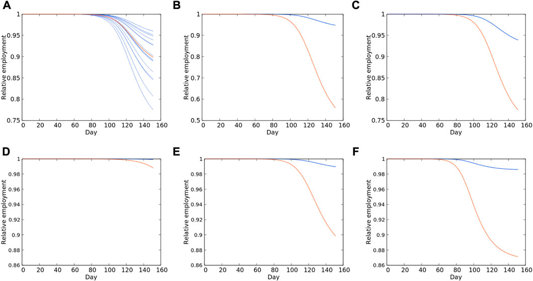
FIGURE 2. Examples of model results using the Fresno SES. Results are for simulations run at R₀ = 2.35, the estimated value on 1 March 2020. All trajectories in each plot are normalized against the initial values in the simulation, and are relative only to the other trajectories in the same plot. (A) Declining sector employments (blue) and total SES employment (red). (B) Employment cascade in the Manufacturing sector, disease-driven (blue) and subsequent cascade (red). (C) Cascades of the Education and Health sector (blue) and Manufacturing sector (red). (D–F)—Disease-driven and employment cascades for R₀ = 2.0, 2.5 and 3.0 respectively.

The divergence, or gap, between the disease-only and economically propagated forecasts—that is, death and severe illness versus cascading job losses—as well as the magnitude of the cascade, are functions of both R₀ and SES network structure, and all the SESs examined exhibited qualitatively similar responses to outbreaks. Losses accumulate over time, but approach limits asymptotically (Figure 2D). The limits of disease-only losses are set by the course of an outbreak and are reached when there are no more susceptible individuals remaining in a population. Those limits in turn set further constraints on the total number of workers lost, including unemployment driven by declines of production, that is, the economic cascade. Cascades grow linearly at low values of R₀, i.e., outbreaks of lower intensity, but accelerate relative to disease-only losses as R₀ increases (Figures 2D–F). Further incremental increases of R₀ eventually lead to abrupt accelerations of cascades, resulting in dramatically greater unemployment than would be predicted by extrapolation from less intense outbreaks (Figure 2F).

3.1.1 Economic tipping points

All SESs in our study exhibit these abrupt accelerations with incremental increases of R₀, or tipping points [21], but differ both at which values of R₀ they transition between regimes of linearly growing cascades to tipping point cascades, as well as the magnitudes of the cascades (Figure 3; Supplementary Figure S3). The tipping point behavior of each system may thus be characterized by the relationship between R₀ and the magnitude of a cascade. Because ΔE*, the gap between an initial loss of workers and the subsequent cascade, asymptotes rapidly with increasing R₀, we summarized the expected reduction of employment in each SES as the growth rate and asymptotic value of ΔE* on day 151 as a function of R₀ (Figure 4). Both values were estimated using a least squares fitted logistic function of E* vs. R₀ profile on day 151 (Figure 4A; Supplementary Table S2). Forecasts of E* ranged from a high of 95.6% of February, 2020 employment (Riverside-San Bernardino-Ontario) to 86.3% (Fresno). E* scales negatively with initial employment and location (Figure 4B), with larger, coastal systems experiencing relatively fewer job losses (Pearson’s correlation, E* and log-transformed E(0), r² = −0.712, p = 0.014, α = 0.05) and slower rates of increasing E* with increasing R₀ (Pearson’s correlation, r² = −0.736, p = 0.01). Neither logistic coefficient, growth rate, or asymptotic value was significantly correlated with SES age structure. The mid-point of the logistic relationship between E* and R₀ (Figure 4A) is the point at which an incremental change of R₀ generates the largest change in the economic cascade. SES mid-points are significantly correlated with the logarithm of system size (Pearson’s correlation, r² = 0.728, p = 0.017) and range from 2.33 to 2.37, with larger SESs having higher thresholds of R₀ (Table 2; Figure 4B) below which the cascading effects of outbreaks are relatively smaller. R₀ of 2.3–2.4 is therefore an economically critical threshold range, or tipping points, for outbreak intensity for the California SESs.

FIGURE 3

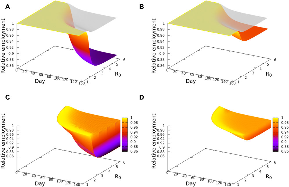
FIGURE 3. (A) Fresno disease-driven (grey) and employment cascades (colored) for R₀ ranging from 0.9 to 4.0. (B) The Los Angeles-Glendale-Long Beach SES. (C) The wedge represents the Fresno gap between disease-driven and economic cascade reductions of employment illustrated in (A), visualizing the magnitude of the cascade. (D) Same visualization as in (C), for the Los Angeles—Glendale—Long Beach SES.

FIGURE 4

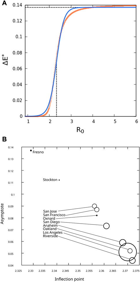
FIGURE 4. (A) Cascade magnitude (red dots), or the difference between disease-driven and economic cascade reductions of employment, on day 151, at values of R₀ ranging from 0.9 to 4.0, for the Fresno SES. Solid blue line is a fitted logistic function. The horizontal dotted line is the asymptotic value of the function. The vertical dotted line is the point of maximum increase of the function (inflection point), showing the corresponding value of R₀. (B) Inflections points and asymptotic values for all SESs, showing that SESs with lower inflection points, that is, critical values of R₀, also experience greater reductions of employment. Symbol size scaled to number of workers per SES.

TABLE 2

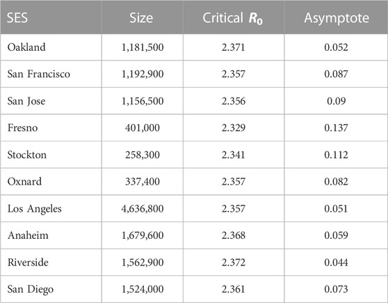
TABLE 2. SES size (number of employees on 1 March 2020), critical values of R₀ (logistic inflection point), and asymptotic cascade value, that is, the fraction of employment reduction as R₀ approaches 4.0.

3.2 System structure

We searched for SES structural features that might explain the dependence of relative unemployment and tipping points on system size using a principal components analysis (PCA) of initial sector employment. SESs were characterized by the number of workers in each sector, and the PCA was performed on the covariance matrix of sector employment per SES. The first two principal components account for 89.6% of the variance, with PC1 being the most important (79.1%). SESs are aligned with PC1 and ordinated significantly according to SES sizes (Pearson’s correlation, SES size and PC1, r² = 0.889, p = 0.0006), but an examination of sector loadings—the contribution of each sector to SES principal component coordinates—shows that it is not size per se that explains the ordination. The Agriculture sector aligns negatively with PC1 (Figure 5), whereas all other sectors align positively (Table 3). This reveals a strong contrast between SESs with relatively large agricultural sectors, compared to non-Agriculture sectors. PC2 ordinates SESs along a spectrum ranging from goods producing sectors, such as Agriculture, and Mining and Logging, to service providing sectors, such as Financial, and Health and Education, but PC2 accounts for significantly less variation (10.5%). The contrast along PC1 is also significantly correlated with the rate at which cascades grow when an SES is perturbed by COVID-19, as illustrated by the thicknesses of the “wedges” in Figure 5 (Pearson’s correlation, growth rate of logistic functions and PC1 coordinates, r² = 0.777, p = 0.0081). This demonstrates that the structure of an SES, or the relative apportionment of workers among industrial sectors, is a primary determinant of the extent to which COVID-19 driven unemployment could cascade through the system.

FIGURE 5

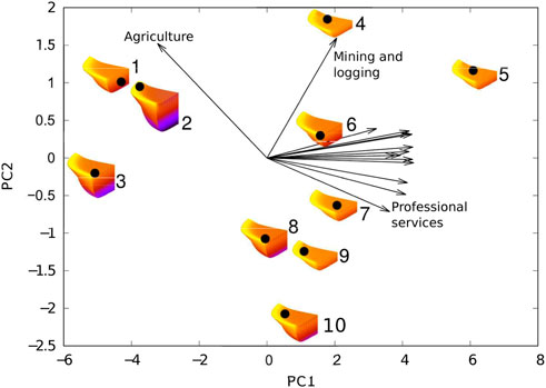
FIGURE 5. Principal components analysis ordination of SESs by employment levels per sector, February, 2020. Each SES is represented by a visualization of its economic cascade under the business-as-usual model, equivalent to examples illustrated in Figures 3C, D. Eigenvector elements represent the contribution of each sector to the ordination and are projected onto the principal component space (arrows), thus explaining sector contributions to relative SES ordination. PC 1 is thus shown to be a contrast between the Agriculture sector and all others, while PC 2 is a gradient of increasing goods producing versus services providing sectors. Arrow length is proportional to the influence of the sector on the ordination. SESs: 1—Oxnard-Thousand Oaks-Ventura; 2—Fresno; 3—Stockton-Lodi; 4—Riverside-San Bernardino-Ontario; 5—Los Angeles-Glendale-Long Beach; 6—San Diego-Carlsbad; 7—Anaheim-Santa Ana-Irvine; 8—San Jose-Sunnyvale-Santa Clara; 9—Oakland-Berkeley-Livermore; 10—San Francisco-San Mateo-Redwood City.

TABLE 3

TABLE 3. Principal components loadings of sectors on the first two principal components.

Structural differences among SESs also illuminate the contributions of relative sector size to total cascade magnitude. The tipping point and maximum unemployment (asymptotic level of previous section) of an SES are dependent on the structure of the SES as revealed by multivariate regression of those values on PC1 scores (multivariate regression of rate and asymptote, Supplementary Table S2, on PC 1; p = 0.004 and p < 0.001 respectively; Supplementary Table S3), with both rate and asymptote declining, or becoming less severe, with increasing PC1 score. Notably, sector sizes within an SES do not account for all the inter-SES variation, as several sectors have no significant relationship between size and cascade unemployment, for example, Retail Trade, Education and Health Services, Leisure and Hospitality, and Other Services. Those sectors have amongst the weakest interactions with other sectors (Figure 1B). In contrast, Manufacturing, which interacts strongly with all sectors, is also the most sensitive to COVID-19 perturbations. There is a significant correlation between sector average interaction strength and the ranking of sectors according to their contributions to the overall SES cascade (Pearson’s correlation, r² = −0.95, p = 0.0001; Spearman’s rank correlation, ρ = −0.878, p = 0.0018). Thus, the response of a sector depends on both the structure of the SES within which it is embedded, including its size and the apportionment of labour among sectors, as well as the strengths of its interactions with other sectors.

3.3 R₀, $R_{\mathtt{e}\mathtt{f}\mathtt{f}}$ and critical thresholds

Specific forecasts of the real world performance of each SES requires a specific set of initial conditions. We therefore extracted from the ensemble simulation results of each SES, the outputs that correspond to the real world R₀ estimate for that SES. Thus, although simulations were performed across a range of potential R₀ values of [0.9, 4.0] to facilitate comparison among SESs, simulations were also performed based on the actual R₀ estimates for each SES, to facilitate comparison between model predictions for an SES to actual employment figures. California R₀ estimates for all the SESs [22] ranged between 1.59 (San Jose-Sunnyvale-Santa Clara) and 2.63 (Stockton-Lodi) at the beginning of March, 2020 (Supplementary Table S1), meaning that initial outbreaks in California would have all sustained positive growth (R₀ > 1). Transmission rates subsequently followed more complicated trajectories because of measures intended to mitigate transmission, as well as variable societal adherence to those measures (Figure 6). Included in the measures were the mandated closures of non-essential workplaces. Thus, effective transmission rates, $R_{\mathtt{e}\mathtt{f}\mathtt{f}}$, are generally lower than the initial transmission rates, R₀. The business-as-usual model shows that reductions of employment, however, are an unavoidable consequence of the disease, even if workplaces remained open (see earlier Results), because losses include workers lost to both the disease, and to the cascading secondary negative economic impacts of those primary casualties.

FIGURE 6

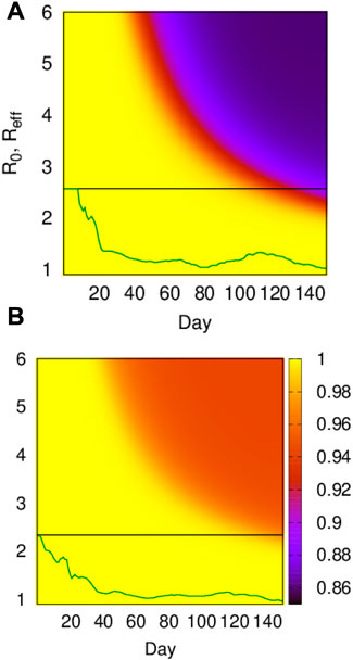
FIGURE 6. (A, B) R₀ and $R_{\mathtt{e}\mathtt{f}\mathtt{f}}$ trajectories superimposed on business-as-usual model forecasts of SES relative employment (colour spectrum). R₀ trajectories (straight black line) indicate model outcome if transmission rates on 1 March 2020 had remained unchanged, whereas $R_{\mathtt{e}\mathtt{f}\mathtt{f}}$ trajectories (green lines) show actual SES histories. (A) Fresno, (B) Los Angeles-Glendale-Long Beach. Note that in both (A, B), the unmitigate R₀ trajdctories would cross the threshold or tipping point (transition between yellow and redder regions) leading to accelerated job losses.

The model also projects what the losses would be at a particular value of R₀ in the absence of mitigating measures. The actual R₀ values of the SESs imply that over time many of the systems would have encountered the tipping points predicted by the model to occur at greater outbreak intensities if transmission rates had remained unchanged or higher $(R_{\mathtt{e}\mathtt{f}\mathtt{f}}\ge R_0)$ (Figure 6). However, the real-world negative divergence of $R_{\mathtt{e}\mathtt{f}\mathtt{f}}$ from R₀ in all the SESs, a direct consequence of mitigation efforts and the reduction of transmission rates, resulted in all systems avoiding the dramatic tipping points and cascades of declining employment predicted by the CASES model (Figure 6).

3.4 The counterfactual scenario

Identifying the complexity and multiple, interrelated factors that underlie the model predictions begs the counterfactual question of how well the economy might have fared if a business-as-usual approach had been adopted. We framed this question on the scale of long-term unemployment (6–12 months) by extending model simulation to 365 days, and using the real-world SES R₀ values. Viewing all the SES’s collectively by summing their model results, total job losses would have reached 720,929 by 1 December 2020, representing a 5.17% reduction relative to 1 March 2020. Of that total, 565,374 would be due not to direct impacts of the disease (severe illness or death), but instead to the cascading effects of declining inter-sector interactions. The model predicts that by March, 2021, those numbers would have grown to a total loss of 756,152 employees, representing 5.43% of total SES employment at the onset of the pandemic (Figure 7A), with 586,185 of those being due to declining inter-sector interactions. As of December, 2020, the true total number of jobs lost in the SESs was actually greater, equalling 983,200 (a 7.1% reduction); according to the simulations, a business-as-usual approach would therefore have spared ≈262,271 jobs.

FIGURE 7

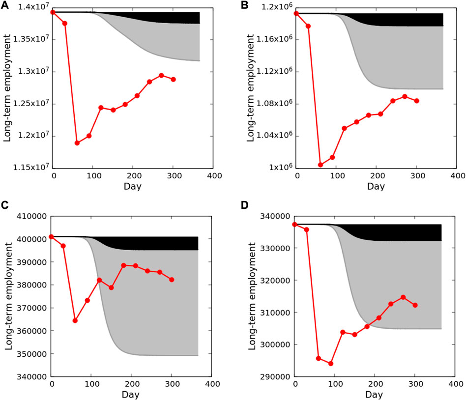
FIGURE 7. Comparisons of unemployment forecast by the business-as-usual model and actual unemployment of March to December, 2020. (A)—all SESs combined; (B)—San Francisco-San Mateo-Redwood City; (C)—Fresno; (D)—Oxnard-Thousand Oaks-Ventura. Actual unemployment is depicted by solid red lines, connecting actual monthly estimates (red circles). Model forecast unemployment of the business-as-usual scenario is the solid grey line, while the red line is actual unemployment. Model unemployment is partitioned between losses to the disease because of death or long-term illness, and unemployment caused by the cascading economic consequences; black and grey filled areas respectively.

The sum of the simulated predictions is lower than unemployment at the height of the Great Recession, when California’s total unemployment surpassed 12% in 2010 [23]. It would nevertheless be among the highest levels of unemployment since the Great Recession. Furthermore, employment by December, 2020 had already recovered substantially from the steep initial losses in every SES between March and April (Figure 7; Supplementary Figure S4). The total proportional loss among all the SESs between March and April, 2020 was 13.54%. Employment began to recover in May, 2020, but the rate of recovery has varied among SESs, and in all cases peaked prior to December, 2020, subsequently declining again.

4 Discussion

The CASES model confirms, for every SES to which it was applied, the hypothesis that severe job loss is an unavoidable outcome of COVID-19 outbreaks. Illness and death of workers reduce sector productivities. The networked nature of the sectors ensures that those primary losses will have cascading effects throughout a system, and that the cascades are system-wide because all sectors are connected.

The magnitude of a cascade depends on four factors. First, the intensity of an outbreak, equivalent here to the initial transmission rate, R₀. The higher the transmission rate, the more workers who become severely ill (or die) and the more rapid the acceleration of a cascade. Second, the age demographics of a sector determine the primary impact of an outbreak on the sector. The greater the number of workers 50 years and older, the greater the primary or direct impact of the disease. Third, although all sectors are connected to each other by supply and demand exchanges, the extent to which the primary impact of an outbreak in one sector will cascade to a secondary impact in another is mediated by the strengths of the exchanges between those sectors. Thus, sectors with stronger interactions will both transmit and receive stronger secondary cascades. Fourth, cascades are affected by the overall structure of an SES, notably the total number of workers, and how those workers are apportioned among sectors (relative sector sizes). The relationships between relative sector sizes and total system size reflect the relatively more dominant role of Agriculture in smaller or inland systems, with an increasing dominance of services-providing sectors as system size and proximity to the coast increase (Figure 5). This reflects the general trend of coastal socio-economic systems in California being both larger than inland systems, and having relatively larger service sectors, such as Information and Financial Services, or larger sectors that are dominated by services, such as Leisure and Hospitality. The trend is significantly correlated with the relative magnitudes of the secondary cascades of job loss, with larger and more service oriented SESs experiencing relatively smaller cascades.

4.1 California job losses

Overall, if COVID-19-driven unemployment in California peaked early in the pandemic, and a potential recovery began during the summer of 2020 [24], then the total unemployment generated by a business-as-usual approach would be less than the real unemployment that was incurred under mitigation conditions (Figure 7A), but by the slim margin of 1.93%. The true cost of a business-as-usual scenario, however, is greater than indicated by this simplistic comparison of model predictions and real unemployment. There are two additional damages that must be considered.

First, unemployment would be distributed disproportionately among the SESs relative to the sizes of their employed populations, and their geographic locations. Real unemployment exceeded model forecasts in most SESs (Supplementary Figure S4), consistent with the overall result explained above. For example, by December, 2020 true unemployment in the San Francisco-San Mateo-Redwood City SES exceeded the model estimate by 15,167 (Figure 7B). Smaller SESs however, which in some instances correspond to California’s inland cities, would in general respond differently. Fresno (Figure 7C), Oxnard-Thousand Oaks-Ventura (Figure 7D) and Stockton-Lodi (Supplementary Figure S4), three systems forecast by the PCA to be most vulnerable to disease-driven cascading unemployment (Figure 5), had actual unemployment levels by August, 2020 lower than model forecasts. This suggests that for those SESs, a business-as-usual scenario would have been worse than the real-world experience. In general, SES responses are variable enough to support the development and application of mitigation policies that pay attention to the variability among SESs based on their size, economic structure, and location. Unemployment generated by a business-as-usual approach would therefore have mixed impact throughout the state, benefiting some regions, while costing others. This is consistent with arguments that at the sub-national level it is important to consider geographically correlated variation when examining the economic impacts of COVID-19 [25].

Second, an unmitigated business-as-usual approach to the disease, while sparing jobs overall, would incur significant losses of life and health. Ultimately, the model’s economic downturns are driven by workers who die or become too ill to continue or return to work, with simulated statewide totals of 155,555 by 1 December 2020, and 169,967 by March, 2021, including 155,088 and 169,450 fatalities respectively. Model unemployment prior to economic cascades is dominated by death because of the disparities of case fatality rates among age categories: a majority of younger workers who contract the disease recover fully, whereas a majority of older workers experience severe illness or death. The totals are also based on workers only, and do not account for illness and mortality in the broader SES populations. As of March, 2021, actual total COVID-19 related deaths in California were fewer, ≈57,000. The business-as-usual approach would therefore, according to the CASES model, have generated additional deaths in excess of 100,000 workers.

In contrast to the un-quantifiable ethical and sociological costs of an unabated pandemic, the economic cost of a business-as-usual policy can be estimated using Value of Statistical Life (VSL) estimates (United States Office of Management and Budget 2003). We used VSL estimates to speculate what the scenario could cost the California economy if employees worked in increasingly risky environments [26]. Various current US Government VSL estimates align roughly at $10 million per person [27]. The estimated cost to the California economy under a business-as-usual scenario would therefore have been $1.55 trillion by December, 2020, increasing to $1.7 trillion by March, 2021, coupled with the 155,088 and 169,450 worker fatalities respectively.

4.2 Model assumptions, limitations and future research

There are several assumptions and nuances of the model that constrain its applicability. First, the model excludes falling consumer demand as a perturbation. Real and anticipated declines of demand certainly affected industries severely, for example, the Leisure and Hospitality sector, which includes travel, restaurants, hotels, museums, and so forth. Our justification for exclusion is that falling demand itself is not a primary outcome of contracting the disease, and that many of the impacts are compounded by the closure and restriction of various industries, for example, travel bans. Nevertheless, even if business had continued as usual, there would be consumer reluctance to participate in certain activities, such as boarding a crowded airplane or cruise ship, or attending a crowded museum. Incorporating those effects into our model would steepen the forecasted job losses, in fact narrowing the gap between the predictions and reality in cases where real unemployment was greater. The “gap” exists because of supply and demand shocks. Recent work measuring those shocks on a national scale [28] suggests that incorporating those factors into our model may become feasible at the regional scale in the near future. Furthermore, initial stock market and industry reactions to anticipated economic downturns add a conservative constraint to our predictions. Those reactions undoubtedly contributed significantly to job losses in California during March-April, 2020. Estimated statewide transmission rates (R₀) were low, ranging between 0.9 and 2.57 [22], and the number of cases (8,233) and deaths (27) were also low [29]. Accelerated job losses and cascading effects to that point were therefore generated by layoffs driven by anticipated declines of economic activity, and not by the disease itself. Nevertheless, although data uncertainty and unavailability mean that model predictions should not be treated as precise numerical predictions, we assert our conclusions are qualitatively accurate.

An additional concern is that we treat SESs as independent entities, when in fact they are parts of an integrated and nested economy at the state, national and global levels. Our analysis shows that there are important structural differences and economic responses among the SESs that would be missed if SESs were aggregated at higher organizational or geographic levels, thus overlooking important issues of scale, geographic and economic heterogeneity that have been highlighted and exacerbated by this disease [25, 30–33]. Nevertheless, given that trade is not limited to isolated SESs, the question arises of what the model dynamics could be were our SESs integrated into the full state and national networks. That analysis is clearly beyond the scope of the current paper, but we can examine the model dynamics and forecasts of aggregated California and total United States systems treated as single SESs. We therefore compiled data for each industrial sector at the California state, and national levels, and simulated the CASES model for each. Interestingly, though perhaps not surprisingly, the dynamics of the total California state SES, although much larger in size than any individual SES, resembles most closely those of its large coastal SESs, such as San Francisco-San Mateo-Redwood City and Los Angeles-Glendale-Long Beach (Figure 8A; Supplementary Figure S4); model forecasts are not as steep as the actual reduction of employment, but the gap narrows considerably during the interval of May-December, 2020. This can be explained by the numerical dominance of the coastal cities in the state SES, the differently structured economies of both the state and cities that feature services prominently, and a gradual acceleration of the model outbreak because of initially low values of R₀. In contrast, the dynamics of the national SES resembles California’s inland and smaller SESs (Figure 8B). This results from both the greater representation of goods production at the national level, as well as the more severe consequences of the disease at the national level, given an R₀ estimate for the country of 4.97 in early March, 2020, compared to the estimate for California of 2.01.

FIGURE 8

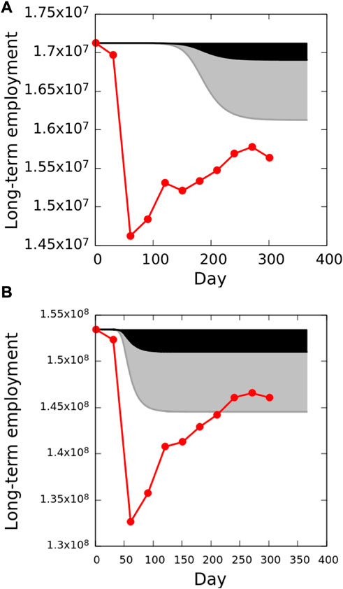
FIGURE 8. Comparisons of unemployment forecast by the business-as-usual model and actual unemployment of March to December, 2020. (A)—California state; (B)—United States. The key to the plots are explained in Figure 7.

Finally, the persistence of COVID-19 suggests two areas of future research. First, there have been multiple waves of varying severity since the initial year of the pandemic. It is possible that extending the counterfactual scenario presented here would suggest longer term economic strategies that could be adopted to better address long-term shocks to socio-economic-health systems. Second, there is the question of whether economic losses, specifically unemployment, affected progression of the disease itself. Such processes would represent feedback from the CASES model to the SIR model. Possible mechanisms facilitating that feedback could be, for example, a slowing of the epidemic because newly unemployed workers would be at a reduced risk of exposure and hence infection. Alternatively, rates of infection could accelerate because those workers might experience greater residential crowding and therefore increased risks of exposure. It is likely that both mechanisms operated in different socio-economic settings. A coupled CASES-SIR model is beyond the scope of the current paper, but presents an interesting avenue of future research.

5 Conclusion

The extent to which economic shutdowns should be implemented to combat outbreaks or resurgence of COVID-19 remains a contentious issue. Here we explored a counterfactual scenario in which California adopted a no shutdown, business-as-usual approach during the first year of the pandemic. Model predictions of job losses for seven large, coastal Californian socio-economic systems with economies dominated by services, such as financial and recreational, were lower than actual job losses. In contrast, smaller and/or more inland systems, where goods production is a larger economic component, are predicted to suffer more under the counterfactual scenario. Overall, California may have experienced lower pandemic-driven unemployment under a business-as-usual approach, but the experience would have been geographically heterogeneous, and it would have come at a cost. Simplistic prioritization of the economy over the health emergency, while possibly lessening economic losses, would nevertheless have resulted in an economic downturn, coupled with greatly increased health consequences of the disease. Fewer jobs would have been lost, but at the expense of the health and lives of tens of thousands of workers. In addition to the moral and societal costs of that impact, future recovery would be hampered by a smaller, younger and less experienced post-pandemic labour force.

The variance of predicted outcomes among SESs subjected to the counterfactual scenario, suggests that combining local structural economic data with dynamic epidemiological and economic models could form a basis for flexible policies going forward that are strategically designed to disrupt the spread of pandemics and simultaneously adhere to the highest and most compassionate moral and societal standards, even while minimizing inevitable economic damage. California eventually developed a county by county re-opening strategy based on positive case counts, an approach that appears to be epidemiologically effective [34]. Our work supports the adoption of similarly nuanced strategies to manage economic impacts.

Data availability statement

The original contributions presented in the study are included in the article/Supplementary Material, further inquiries can be directed to the corresponding author.

Author contributions

PR, MA, DG, and JR designed the project. MA researched primary economic and epidemiological data. PR developed the mathematical model, and conducted statistical analyses. PR and JR conducted simulations. JR developed the online interactive simulation. PR, MA, DG, and JR contributed to writing of the manuscript. All authors contributed to the article and approved the submitted version.

Funding

This study was supported by US National Science Foundation Grant 2032769 to PR.

Acknowledgments

The authors thank Ted Burczak, Katie Jewitt, Skylar Knight and two reviewers for helpful comments. The authors acknowledge that the California Academy of Sciences occupies land that is the ancestral homeland of the Ramaytush-Ohlone, the vast majority of whom were forcibly removed from their homelands. We acknowledge this painful history and honor their legacy and continuing contributions to better understanding the history and present of the United States.

Conflict of interest

The authors declare that the research was conducted in the absence of any commercial or financial relationships that could be construed as a potential conflict of interest.

Publisher’s note

All claims expressed in this article are solely those of the authors and do not necessarily represent those of their affiliated organizations, or those of the publisher, the editors and the reviewers. Any product that may be evaluated in this article, or claim that may be made by its manufacturer, is not guaranteed or endorsed by the publisher.

Supplementary material

The Supplementary Material for this article can be found online at: https://www.frontiersin.org/articles/10.3389/fphy.2023.1074704/full#supplementary-material

References

1. Bank W. The global economic outlook during the covid-19 pandemic: A changed world. Washington, DC, USA: World Bank Feature Story (2020).

Google Scholar

2. Pak A, Adegboye OA, Adekunle AI, Rahman KM, McBryde ES, Eisen DP. Economic consequences of the Covid-19 outbreak: The need for epidemic preparedness. Front Public Health (2020) 8:241. doi:10.3389/fpubh.2020.00241

PubMed Abstract | CrossRef Full Text | Google Scholar

3. Reicher S, Stott C. On order and disorder during the Covid-19 pandemic. Br J Soc Psychol (2020) 59:694–702. doi:10.1111/bjso.12398

PubMed Abstract | CrossRef Full Text | Google Scholar

4. Duncan TK, Redford A. How shutting down the economy much longer could kill tens of thousands of Americans (2020). Available from: https://thefederalist.com/2020/03/30/how-shutting-down-the-economy-much-longer-could-kill-tens-of-thousands-of-americans/ (Accessed November 14, 2022).

Google Scholar

5. Starr W. Counterfactuals. In: EN Zalta, editor. The stanford encyclopedia of philosophy. Summer 2021 edn. Stanford, CA, USA: Metaphysics Research Lab, Stanford University (2021).

Google Scholar

6. Corcoran K. California’s economy is now the 5th-biggest in the world, and has overtaken the United Kingdom. New York City: Business Insider (2018). Available from: https://www.businessinsider.com/california-economy-ranks-5th-in-the-world-beating-the-uk-2018-5 (Accessed November 19, 2020).

Google Scholar

7.OMB. Omb bulletin no. 20-01 (2020). Available from: https://tinyurl.com/y7oz7sfy (Accessed November, 19, 2020).

Google Scholar

8.CAEDD. Labor market information for metropolitan areas (2020). Available from: https://tinyurl.com/yaeync44 (Accessed June 17, 2020–May 26, 2021).

Google Scholar

9. Lever JJ, van Nes EH, Scheffer M, Bascompte J. The sudden collapse of pollinator communities. Ecol Lett (2014) 17:350–9. doi:10.1111/ele.12236

PubMed Abstract | CrossRef Full Text | Google Scholar

10. Roopnarine PD, Angielczyk KD. Community stability and selective extinction during the Permian-Triassic mass extinction. Science (2015) 350:90–3. doi:10.1126/science.aab1371

PubMed Abstract | CrossRef Full Text | Google Scholar

11. Jiang J, Huang ZG, Seager TP, Lin W, Grebogi C, Hastings A, et al. Predicting tipping points in mutualistic networks through dimension reduction. Proc Natl Acad Sci (2018) 115:E639–E647. doi:10.1073/pnas.1714958115

PubMed Abstract | CrossRef Full Text | Google Scholar

12. Meng Y, Grebogi C. Control of tipping points in stochastic mutualistic complex networks. Chaos: Interdiscip J Nonlinear Sci (2021) 31:023118. doi:10.1063/5.0036051

CrossRef Full Text | Google Scholar

13. Arrow KJ, Ehrlich PR, Levin SA. Some perspectives on linked ecosystems and socio-economic systems. In: Environment and development economics: Essays in honour of sir partha dasgupta. Oxford, UK: Oxford University Press (2014). p. 95–116.

CrossRef Full Text | Google Scholar

14.USBLS. Monthly employment situation report: Quick guide to methods and measurement issues (2020). Available from: https://www.bls.gov/bls/empsitquickguide.htm (Accessed November 24, 2020).

Google Scholar

15.USBLS. Technical notes for the current employment Statistics survey (2020). Available from: https://tinyurl.com/y7bzsy7s (Accessed December 10, 2020).

Google Scholar

16. Easley D, Kleinberg J. Networks, crowds, and markets. Cambridge, UK: Cambridge Books (2012).

Google Scholar

17. Acemoglu D, Akcigit U, Kerr W. Networks and the macroeconomy: An empirical exploration. Nber Macroeconomics Annu (2016) 30:273–335. doi:10.1086/685961

CrossRef Full Text | Google Scholar

18. McNerney J, Fath BD, Silverberg G. Network structure of inter-industry flows. Physica A: Stat Mech its Appl (2013) 392:6427–41. doi:10.1016/j.physa.2013.07.063

CrossRef Full Text | Google Scholar

19. Xu M, Liang S. Input–output networks offer new insights of economic structure. Physica A: Stat Mech its Appl (2019) 527:121178. doi:10.1016/j.physa.2019.121178

CrossRef Full Text | Google Scholar

20. Leontief W, Fabricant S, Friend I, Koopmans T, Morgenstern O, Jacobs W, et al. Input-output analysis and its use in peace and war economics. Am Econ Rev (1949) 5:211–25.

Google Scholar

21. Lenton TM. Tipping points in the climate system. Weather (2021) 76(10):325–6. doi:10.1002/wea.4058

CrossRef Full Text | Google Scholar

22.CalCAT. Current R-effective in California (2020). Available from: https://calcat.covid19.ca.gov/cacovidmodels/ (Accessed August 26, 2020, August 27, 2020, October 2, 2020).

Google Scholar

23.CAEDD. California unemployment drops to an even 11 percent in September (2020). Available from: https://tinyurl.com/yaxhkwab (Accessed November 24, 2020).

Google Scholar

24. Schniepp M. Status of the recovery/summer 2020 (2020). Available from: https://californiaforecast.com/july-2020/ (Accessed December 10, 2020).

Google Scholar

25. Polyakova M, Kocks G, Udalova V, Finkelstein A. Initial economic damage from the Covid-19 pandemic in the United States is more widespread across ages and geographies than initial mortality impacts. Proc Natl Acad Sci (2020) 117:27934–9. doi:10.1073/pnas.2014279117

PubMed Abstract | CrossRef Full Text | Google Scholar

26. Viscusi WK, Aldy JE. The value of a statistical life: A critical review of market estimates throughout the world. J Risk Uncertainty (2003) 27:5–76. doi:10.1023/a:1025598106257

CrossRef Full Text | Google Scholar

27. Greenstone M, Nigam V. Does social distancing matter? Chicago, IL, USA: University of Chicago, Becker Friedman Institute for Economics Working Paper (2020).

Google Scholar

28. del Rio-Chanona RM, Mealy P, Pichler A, Lafond F, Farmer JD. Supply and demand shocks in the COVID-19 pandemic: An industry and occupation perspective. Oxford Rev Econ Pol (2020) 36:S94–S137. doi:10.1093/oxrep/graa033

CrossRef Full Text | Google Scholar

29.Johns Hopkins School and Medicine. Coronavirus resource center. Baltimore, Maryland: Johns Hopkins School and Medicine (2020). Available from: https://coronavirus.jhu.edu/ (Accessed May 18, 2020).

Google Scholar

30. Mena GE, Martinez PP, Mahmud AS, Marquet PA, Buckee CO, Santillana M. Socioeconomic status determines Covid-19 incidence and related mortality in santiago, Chile. Science (2021) 372:eabg5298. doi:10.1126/science.abg5298

PubMed Abstract | CrossRef Full Text | Google Scholar

31. Andrasfay T, Goldman N (2021). Reductions in 2020 us life expectancy due to Covid-19 and the disproportionate impact on the black and latino populations. Proc Natl Acad Sci 118, e2014746118, doi:10.1073/pnas.2014746118

PubMed Abstract | CrossRef Full Text | Google Scholar

32. Chang S, Pierson E, Koh PW, Gerardin J, Redbird B, Grusky D, et al. Mobility network models of Covid-19 explain inequities and inform reopening. Nature (2021) 589:82–7. doi:10.1038/s41586-020-2923-3

PubMed Abstract | CrossRef Full Text | Google Scholar

33. Diffenbaugh NS, Field CB, Appel EA, Azevedo IL, Baldocchi DD, Burke M, et al. The Covid-19 lockdowns: A window into the Earth system. Nat Rev Earth Environ (2020) 1:470–81. doi:10.1038/s43017-020-0079-1

CrossRef Full Text | Google Scholar

34. Karatayev VA, Anand M, Bauch CT. Local lockdowns outperform global lockdown on the far side of the COVID-19 epidemic curve. Proc Natl Acad Sci (2020) 117:24575–80. doi:10.1073/pnas.2014385117

PubMed Abstract | CrossRef Full Text | Google Scholar