 Joia M. Miller
 Daniel L. Blair
 Jeffrey S. Urbach
- Department of Physics and Institute for Soft Matter Synthesis and Metrology, Georgetown University, Washington, DC, United States
We introduce a novel approach to reveal ordering fluctuations in sheared dense suspensions, using line scanning in a combined rheometer and laser scanning confocal microscope. We validate the technique with a moderately dense suspension, observing modest shear-induced ordering and a nearly linear flow profile. At high concentration (ϕ = 0.55) and applied stress just below shear thickening, we report ordering fluctuations with high temporal resolution, and directly measure a decrease in order with distance from the suspension’s bottom boundary as well as a direct correlation between order and particle concentration. Higher applied stress produces shear thickening with large fluctuations in boundary stress which we find are accompanied by dramatic fluctuations in suspension flow speeds. The peak flow rates are independent of distance from the suspension boundary, indicating that they likely arise from transient jamming that creates solid-like aggregates of particles moving together, but only briefly because the high speed fluctuations are interspersed with regions flowing much more slowly, suggesting that shear thickening suspensions possess complex internal structural dynamics, even in relatively simple geometries.
1 Introduction
Flowing dense suspensions of colloidal particles appear in a wide range of important industrial processes, and the presence of flow can dramatically modify the suspension microstructure, which in turn impacts flow properties (reviewed in [1–3]). In particular, the presence of simple shear modifies the well-understood phase behavior of dense suspensions of nearly monodisperse colloidal particles in equilibrium. Modest shear promotes layering which enhances crystallization, while higher shear rates often disrupt crystalline order [1, 3–8]. In addition, the bulk response of the suspension can be very sensitive to the material close to the confining boundaries [9–12]. Planar boundaries promote the formation of layers of particles parallel to the boundaries [9, 13], enabling more efficient shearing as layers slide past each other with reduced close particle interactions, and a resulting reduction in the local viscosity [14–16]. The layering also enhances ordering within the layer, and in many circumstances the sliding layers show a high degree of hexagonal ordering, similar to what is seen in two dimensional colloidal crystals [12, 17]. In many dense suspensions, the shear thinning arising from increased layering is followed by dramatic shear thickening when the applied stress exceeds a critical value, with the increase in viscosity attributable to a transition from primarily hydrodynamic particle interactions at low stress to frictional interactions at high stress (reviewed in [18]). The onset of frictional interactions will likely disrupt layering [19], a scenario confirmed by recent computer simulations [20]. A variety of evidence suggests that strong shear thickening is accompanied by complex spatiotemporal dynamics, including fluctuations in flow speed, local stress, and particle concentration [21–35]. These results highlight the need for methods that can probe the dynamics of dense colloidal suspension with high spatial and temporal resolution. Here we introduce a new approach to assessing dynamic ordering using a combined rheometer and laser scanning confocal microscope [35], where the laser scanning is limited to one spatial direction. In this case the scan is perpendicular to the flow direction, and the suspension flow is primarily responsible for the temporal evolution of the recorded intensity. We validate the technique using a moderately dense suspension (volume fraction ϕ = 0.52), where only modest shear-induced ordering is observed. At higher concentration (ϕ = 0.55) and applied stress just below the onset of shear thickening, we measure ordering fluctuations with high temporal resolution, and directly measure the decrease in ordering with distance from the bottom boundary of the suspension. We also observe a direct correlation between ordering and particle concentration, with local regions of high order corresponding to high particle concentrations, consistent with recent observations from computer simulations [20]. Higher applied stress produces shear thickening, and we find that the large fluctuations in boundary stress that underlie thickening are accompanied by dramatic fluctuations in suspension flow rates. The peak flow rates are independent of distance from the suspension boundary, indicating that they arise from transient jamming that creates solid like aggregates of particles moving together. Such aggregates must be short-lived because the high speed fluctuations are interspersed with regions flowing much more slowly, suggesting that shear thickening suspensions possess very complex internal structural dynamics, even in relatively simple geometries.
2 Approach
For particulate suspensions, particle velocities are often extracted from image sequences by particle tracking or correlation analysis (PIV) [36]. Particle tracking typically requires that the time between images is small compared to the time for a particle to move an interparticle separation (so that each particle can be unambiguously identified in successive images). Thus for a frame rate f and an interparticle spacing δ, the flow speed must satisfy
We use an alternative approach here, inspired by fluid dynamics and machine vision applications where the motion of material past point or line detectors is used to infer speeds and structure [37, 38]. We take advantage of the rapid scan rate of a laser scanning confocal microscope, where the point of focus is rapidly scanned back and forth in one direction, which we will call the x axis, with the normal rastering perpendicular to the scan line in the focal plane disabled (Figure 1A). We illustrate the principle with a simple example: A fluorescent particle transiting the line will produce a local intensity extremum, from which its x position can be determined. The time it takes the particle to transit the line can be measured by the length of the ridge produced when a position-time intensity surface is generated (Figure 1B). If the center of the particle is in the plane of focus and neglecting the effects of the finite optical resolution, the magnitude of the component of the particle velocity perpendicular to the line can be determined as v = D/T, where D is the particle diameter and T the transit time. The requirement that the transit time is long compared to the time between scans means that the flow speed must be
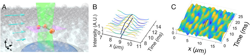
FIGURE 1. (A) Schematic of linescan imaging of a sheared dense suspension. The illumination laser rapidly scans back and forth, focused along the green line. Particles transiting the line are illuminated (orange). The imaging region for the usual 2D laser scan is indicated by the dashed line, and the arrows represent the average velocity field of the sheared suspension. The depth of focus (effective width of the image plane in z) depends on the optical setup, and is
The situation sketched above describes motion advection purely in the direction of the shear flow, but the linescan measurement will also be affected by other components of the flow velocity. Because of the geometry, the speed in the flow direction will normally be of order
A related approach has been used to measure flow profiles in capillary and microfluidic systems (reviewed in [39, 40]) where fluorescence correlation spectroscopy (FCS) is employed to extract speeds using fluorescent single molecules or nanoparticles [41]. The exact shape of the intensity autocorrelation function depends on the relative importance of diffusion and advection, but when diffusion is negligible compared to advection (as is the case in the situations considered here), the intensity autocorrelation function is a Gaussian with a width determined by the flow speed and the size of the illumination volume [42]. By varying the scan orientation relative to the flow direction, the full (average) three dimensional velocity vector can be determined [43, 44]. In those applications, however, the volume fraction of the fluorescent species is always low, so they are reasonably assumed to be distributed randomly. In the results presented below, spatial ordering dramatically affects the spatiotemporal intensity fluctuations, complicating the determination of the flow speed but revealing novel behavior in dense colloidal shear flow.
Validation: To verify the accuracy of the linescan approach under these conditions, we performed tests on a moderately dense suspension, volume fraction ϕ = 0.52, where the viscosity is only weakly non-Newtonian, under constant shear rate conditions. Figure 2 shows three representative kymographs, each generated from 512 scans (65 ms total time), showing the range of speeds from the slowest (
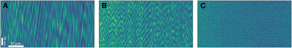
FIGURE 2. Representative space-time kymographs generated from linescans (horizontal) stacked vertically taken in a sheared dense suspension of silica particles of diameter 1 μm, ϕ = 0.52, at different shear rates. The spheres are not fluorescent, and a fluorescent dye is added to the solvent. (A)
We acquired a series of 900 kymographs at heights above the bottom boundary of z = 3, 6, 10, 20μm, for constant applied shear rates of
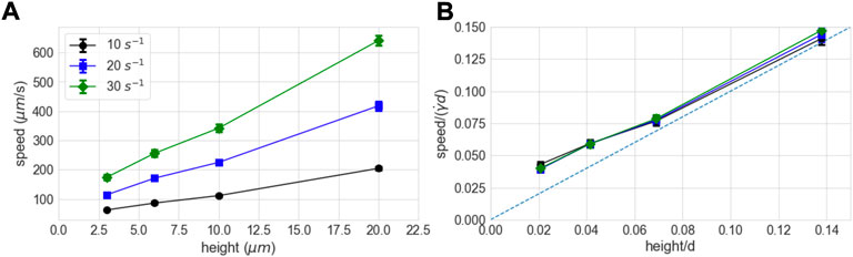
FIGURE 3. (A) Flow profiles for constant shear rate generated from linescan data at different heights (ϕ = 0.52), at different constant shear rates. (B) Particle speeds scaled by the speed of the top plate of the rheometer,
3 Results
Here we report the results of a dense suspension of 1 μm silica spheres at a volume fraction ϕ ≈ 0.55. The flow curve from bulk rheology for this sample is shown in Figure 4, and exhibits behavior similar to previous reports of shear thickening in similar systems [18], and in particular matches that of our previous results measuring local boundary stress fluctuations of the same system [35]. The viscosity shows substantial shear thinning (viscosity decreasing as applied shear stress is increased) until a critical stress of σc ≈ 20 Pa, at which point strong shear thickening is observed. The transition occurs at a shear rate of
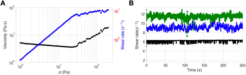
FIGURE 4. (A) Viscosity (○) and shear rate (■) as a function of applied shear stress for the suspension used in this study, composed of silica particles of diameter 1.0 μm, ϕ ≈ 0.55. (B) Representative plots of shear rate vs time for a constant applied stress of 20 (bottom), 50 (middle) and 100 (top) Pa. Specifically, the time series shown correspond to the kymographs reported at z = 3 μm.
3.1 Order and density fluctuations before the onset of shear thickening
As summarized in Section 1, the shear thinning observed for applied stress σ < σc is generally attributed to shear induced ordering, where organization of the monodisperse spheres into layers, and hexagonal ordering with the layers, reduces the viscosity by reducing collisions as the layers slide past one another. Figure 5 shows representative kymographs at σ = 20 Pa, at three different heights. At z = 3 μm above the bottom surface, the kymograph (top) reveals a very regular hexagonal lattice, elongated along the time axis because the particle speed is relatively small. Defects in the hexagonal order tend to be extended in the flow (time) directions, e.g. at the top right of the panel. The left side of the kymograph shows a region of relatively low order, which is uncommon at this height, as quantified below. At z = 10 μm (middle), regions of hexagonal order show up as small islands in a sea of disorder, with a tendency to be longer in the time direction than in the spatial (vorticity) direction. Particle extent and separations in the time direction are proportional to the flow speed, so comparing dimensions requires rescaling by the flow speed (Supplementary Figure S1), or, more simply, counting the number of particle diameters in the different directions. The interpretation of the kymographs as direct images of 2D particle arrangements presumes that the rate of particle rearrangement is relatively slow compared to the rate at which structures traverse the scan region. The persistence of the hexagonal order suggests that this is a reasonable approximation.
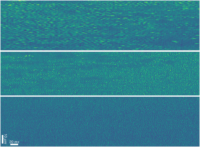
FIGURE 5. Representative space-time kymographs generated from linescans (vertical) stacked horizontally at 20 Pa constant applied stress at heights of 3 μm (top), 10 μm (middle), and 20 μm above the bottom surface. Each image consists of 4,096 scans, for an elapsed time of 520 ms (Note that the orientation is different than Figure 2, with time on the horizontal axis).
In addition to revealing the existence and shape of small islands of order, the kymographs show that the ordered regions are darker than regions of disorder. This can be seen clearly in the islands present at z = 10μm, where the overall intensity is lower in the islands than around them (Figure 5, middle), but is also evident at z = 3 μm (top), where the small regions of disorder are brighter than their surroundings. Because the fluorescent dye is in the solvent, brighter regions correspond to a lower concentration of colloidal particles. Below we quantify the correlation between order and low intensity, and show that is substantial at all heights at 20 Pa applied stress. This observation is consistent with simulations of dense suspensions of monodisperse particles, where a correlation between local ordering and high particle concentration was observed [20].
Quantifying the degree of hexagonal order in the kymographs is complicated by several factors. The images generated by individual particles depend on the height of the particle relative to imaging position. As discussed above, the particles tend to order in layers, and the patterns will be different when the center of the particle layer is at the linescan height compared to when the space between the layers aligns with the scan. A further complication arises from the fact that the 1 μm diameter of the particles is only a little larger than the resolution of the optical microscope, so particle images are not well separated. Finally, the distortion of the image in the flow direction depends on the speed of the flow, which fluctuates in time. Despite these complications we have found that we can extract a robust quantitative measure of the flow speed and order in each kymograph by calculating the two-dimensional intensity autocorrelation function,
Figure 6 shows a portion of the timeseries of speed, C6, and average intensity generated from kymographs at z = 10 μm. The first eight points in the time series correspond to the image shown in Figure 5 (middle). The decrease in order in the image (moving right to left) shows as a decrease in C6 from
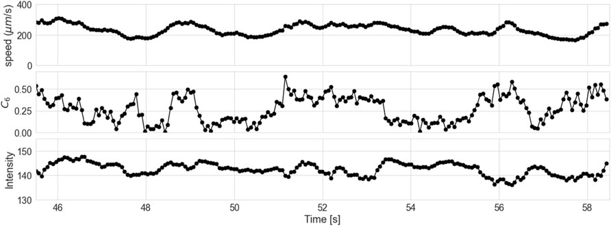
FIGURE 6. Section of time series of speed, hexagonal order, and intensity generated from kymographs at applied stress 20 Pa and height 10 μm. The first eight data points correspond to the image shown in Figure 5 (middle).
A modest positive correlation can be observed between order and speed, which is consistent with an ordering-induced increase in local velocity close to the wall, but is complicated by the fact that the correlation analysis used to determine the flow speed likely has a weak dependence on order (see Methods). Finally, we note that the orientation of the hexagonal order is such that intensity peaks and valleys always align in the flow direction, corresponding to a phase angle for the complex order parameter
The change in flow speed and order with distance from the bottom surface can be seen most clearly from histograms, as shown in Figure 7. The speeds increase with height, as expected, with a significant increase in the spread of speeds that is roughly proportional to the speed increase. Specifically, the ratio of the standard deviation to the mean speed is {0.14, 0.19, 0.21, 0.17} for heights z = {3, 6, 10, 20}μm, respectively. The slightly higher fractional spread at 6 and 10 μm likely arises from the coupling between order and speed mentioned above. The change in order with height is much more dramatic, showing uniformly high order 3 μm above the bottom surface, occasional disordered regions at 6μm, roughly equal order and disorder at 10μm, and mostly disordered at 20 μm. This behavior is summarized in Figure 8, which shows the average and standard deviations for speed and order as a function of height. Figure 8 also includes the data from 50 Pa applied stress, which shows very similar trends. The increase in curvature of the flow profile close to the boundary indicates a lower local viscosity. Boundary-induced ordering and an associated viscosity decrease in dense suspensions has been seen previously, but the high speed imaging approach used here enables us to quantify spatio-temporal fluctuations in previously inaccessible regimes.
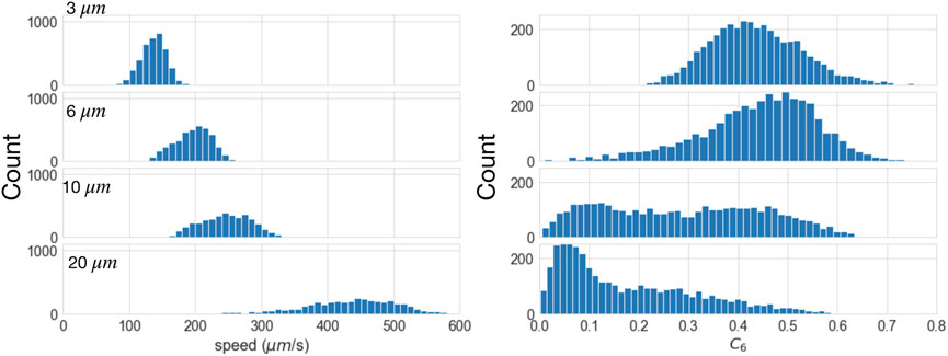
FIGURE 7. Histograms of speed and order generated from kymographs at applied stress 20 Pa (Each height: 3,900 kymographs, 65 ms each).
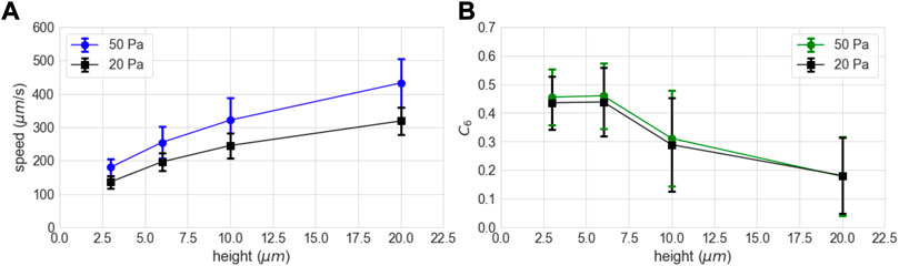
FIGURE 8. Profiles of average velocity (A) and order (B) for 20 and 50 Pa applied stress. Error bars are standard deviations (N = 3,900).
3.2 Fluctuations associated with shear thickening
At higher applied stresses, the suspension shows substantial shear thickening and the nature of the fluctuations change dramatically. We have previously shown that shear thickening is associated with large fluctuations in stresses at the boundary of the sheared suspension [31–35], and specifically for the particles used here shear thickening is associated with a proliferation of the regions of high stress that propagate in the flow direction with approximately half the speed of the top plate
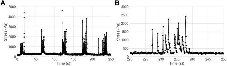
FIGURE 9. (A) Boundary stress (component in the flow direction) for 100 Pa applied stress. (B) Expanded view of one cluster of events from data shown in (A).
Figure 10 shows the velocity time series for four different heights at 100 Pa applied stress. The clustering of intermittent events is consistent in every data set (Each time series is a different measurement run, and is different from the run that produced the boundary stress shown in Figure 9.) Thus we can be confident that the intermittent spikes in speed represent the flow fluctuations that are associated with the intermittent high boundary stress spikes. Interestingly, the spacing between the clusters,
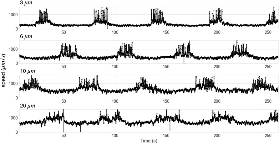
FIGURE 10. Full timeseries of speeds for 100 Pa applied stress at heights of 3, 6, 10, and 20 μm.
Figure 11 shows the time series for a cluster of spikes at each observed height, with the time axis shifted so that in each set the spikes start at the same time. The kymograph at the top of the figure, showing a single speed spike at z = 3μm, indicates that before the spike, the particles exhibit a high degree of hexagonal ordering, consistent with the behavior observed at this height at lower applied stress. The transition to high speed flow is evidenced by a remarkably sharp boundary that extends primarily along the vorticity direction, but with some meandering in the flow direction, consistent with the fluctuations in boundary stress reported previously [35]. A complete absence of ordering and a significant increase in average intensity marks the period of high speed flow, suggesting a region of reduced particle concentration, although there are correlations between speed and intensity introduced by the instrumentation, and further calibration will be required to separate measurement effects from concentration when the speed variation is large. The transition back to lower speed flow is also quite rapid, but the hexagonal ordering takes longer to recover. These features are consistent across the high speed events, as shown by the time series of speed, c6, and intensity at 3 μm (Supplementary Figure S2).
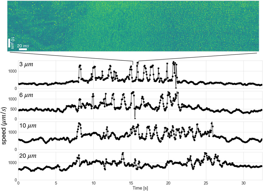
FIGURE 11. Timeseries of speed for 100 Pa applied stress at heights of 3, 6, 10, and 20 μm during one burst of high speed events. The image shows a kymograph from a single event. The initial times are shifted so the bursts start at approximately the same time.
Also evident in Figure 10 is that the speed differential between the spikes and the background is smaller at larger z, indicating that the events represent a more dramatic speed-up close to the bottom boundary. Finally, the clusters appear to be more spread out at larger z. Since the periodicity is independent of z, the propagation speed of the clusters should be independent of z, so the spreading of the clusters with height suggests that the spatial extent of the region of high stress increases with depth.
We can use the clustering of high speed events in the velocity time series to quantify the region of “normal” flow, away from the events (the specific segmentation is shown in Supplementary Figure S3). Figure 12A shows the flow profile obtained during those time periods, and the overall shape closely matches that seen at lower stresses (Figure 8). The agreement is made more evident by scaling the measured speeds by the average shear rate as reported by the rheometer (Figure 12B), where all three profiles overlap, with no free parameters. Something very different happens during the high speed events. We find empirically that selecting the highest 60 speeds from the 3,900 measurement points provides a reasonable measure of the peak speeds during the high speed events (Supplementary Figure S4), and we find that the average of those top speeds is nearly height independent (Figure 12). Scaling the peak speeds by average the speed of the top plate shows that the height-independent speed is on the order of vp, consistent with a solid jammed aggregate moving with the speed of the top plate, perhaps with some slip (Note however, as discussed below, that the high speed events are quite likely associated with substantial non-affine flows, and thus it is possible that flows in the gradient direction contribute to the decay of the correlation and thus to the calculated speed.) Imaging of the bottom layer of particles confirms that the high speed fluctuations are associated with large slip of that layer. Those apparent aggregates are intertwined with regions of the suspension where the particles are flowing much slower (Figure 11), which is inconsistent with a single solid aggregate. These results provide the first direct measurements of the structure of the velocity field inside of high stress fluctuations in shear thickening suspensions.
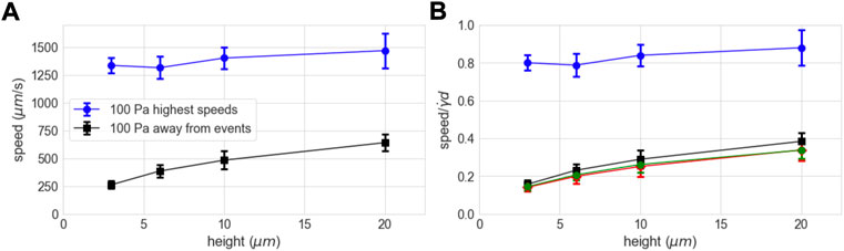
FIGURE 12. (A) Average speed at different heights from portions of the time series away from the high speed events, and average speed for the highest speeds in each time series (N = 60). (B) Data in (A) scaled by the speed of the top plate, with the scaled profiles from 20 to 50 Pa for comparison (Figure 8A).
4 Discussion
4.1 Order and concentration fluctuations before the onset of shear thickening
The dynamics revealed by high speed linescan imaging presented above are consistent with previous observations of boundary induced ordering in sheared dense monodisperse suspensions, but provide a more detailed picture of the spatiotemporal dynamics and demonstrate the presence of a strong connection between ordering and concentration fluctuations. Planar boundaries enhance layering in colloidal suspensions, and the layering can reduces viscous dissipation, producing shear banding [12, 16, 20]. Hexagonal ordering of monodisperse particles within layers of sheared suspension has also been seen in a variety of circumstances, starting with the seminal work of Ackerson and coworkers [4, 45]. Particularly relevant to this work, an imaging study by Wu et al. observed fluctuation in hexagonal ordering during the process of shear-induced melting in a confined suspension arising from the nucleation of localized domains that temporarily lost and regained their ordered structure [6]. Similar behavior has been reproduced in computer simulations [12, 17]. Recent simulation results reported that defects in crystalline order are associated with local decrease in particle concentration [20]. It is perhaps not surprising that the interplay between shear flow, crystal nucleation, and shear-induced crystal breakup produces a complex phase diagram with complex dynamics [3]. Here we show that for a monodisperse suspension at high packing fraction and high Peclet number (Pe ∼ 50Figure 60), the transition from mostly ordered to mostly disordered occurs
4.2 Fluctuations associated with high local stresses during shear thickening
The high speed imaging approach employed here has revealed that localized high boundary stresses are accompanied by large rapid speed increases near the boundary, as well as a loss of order (Figure 11). Recent simulation results showed that the transition from hydrodynamic to frictional interparticle interactions that is believed to underlie strong shear thickening [18] is associated with a disruption of layering and ordering [20]. It seems likely that we are observing a similar transition, from relatively low stress, lubricated particle interactions producing layered, ordered low viscosity flow, to high stress, frictional particle interactions producing high viscosity disordered flow in the regions that produce high boundary stress. This transition appears to be remarkably sharp, with a boundary that is only a few particles wide (Figure 11, top). Also remarkable is the observation that the particle speeds during these events are independent of depth (Figure 12). This suggests that the particles are moving together, as a jammed aggregate, similar to the model proposed to explain propagating high normal stresses observed in cornstarch suspensions [29]. It is important to note, however, that the linescan measurements performed here do not distinguish between flow components perpendicular to the scan direction (i.e. in the flow or gradient directions). As discussed above, under usual flow conditions the component of the velocity in the flow direction, of order
More generally, measurements of nearly affine flow away from the localized high stresses, both in this system and in cornstarch [34], combined with the rapid fluctuation in velocity measured during the clusters of events (Figure 11), suggests a complicated flow field. Furthermore, although instrumental effect preclude a direct measurement of particle concentration during the high speed events, the longstanding connection between frictional interactions and dilatancy [18], evidenced by our observation of fluid migration associated with high stress fluctuations in cornstarch suspensions [34], suggests that relative flow between the particulate and fluid phases likely plays an important role in the observed speed fluctuations.
These observations contribute to a growing body of evidence indicating that the shear thickening transitions typically involved complex spatiotemporal dynamics with structures propagating in the flow direction, including dilatant fronts [23, 25], local deformations of the air-sample interface at the edge of the rheometer tool [26, 30], local normal stresses in sheared cornstarch [29], concentration fluctuations appearing as periodic waves moving in the direction of flow [28], and high shear stress at the suspension boundary [31, 32, 34, 35]. The specifics of the dynamics vary considerably, presumably indicating a sensitivity to the details of the suspension and the measurement geometry. This sensitivity is perhaps not surprising, given that shear thickening involves instabilities that can produce discontinuities in material parameters. The location of those discontinuities in a uniform extended system represent a broken symmetry, and thus in any physical realization will be very sensitive to the parameter variations (e.g. of shear rate, rheometer gap, distance from suspension boundary) that are present in all experimental systems.
Here we have presented an initial application of a powerful new approach that reveals spatiotemporal dynamics of sheared dense suspensions with high spatial and temporal resolution. With further testing and validation the approach has the potential to provide accurate and precise measurements of local speed, structure, and particle concentration, and should provide a new avenue to answer open questions about dense suspensions under flow.
5 Methods
All experimental suspensions were composed of 0.9 μm silica beads (Bang’s Lab) in an index-matched (80/20 v/v) glycerol/water mixture. For imaging purposes, fluorescein sodium salt was added to the suspension so that the unlabeled spheres could be imaged as dark spots in a fluorescent background. Rheological measurements were performed on a stress-controlled rheometer (Anton Paar MCR 301) mounted on an inverted confocal (Leica SP5) microscope [35] using a cone-plate geometry with a diameter 25 mm. The linescan data was acquired with a ×60 objective at a radius of 2/3 of the plate diameter, where the rheometer gap is d ≈ 145 μm.
Linescan analysis: A typical data set is composed of a one to two million scans, with the scan direction aligned along the vorticity axis (perpendicular to the flow and the gradient). For visualization, we typically divide the set into a series of 2D arrays, with one dimension (horizontal) given by the number of pixels per scan (here 1,024), and the other dimension (vertical) given by the chosen number of scans per image, in this case 512 scans. Figure 14A shows an example image generated from 1 μm diameter non-fluorescent spheres in a fluorescent bFigure 5ackground, 10 μm above the bottom of the sheared suspension, similar to those shown in Figure 5. Individual particles show up as dark ovals. In principle, the vertical axis of each oval could be used to measure the speed of each particle. In practice, in many places identifying individual particles is challenging, and we have found correlation analyses more reliable (This arises in part because we have no control of the position of particles relative to the plane of focus, and the image will include contributions from particles that are
One approach to extract a characteristic transit time from the linescan intensity data, I (x, t), is to calculate the autocorrelation in the time direction, g (Δt) = <δI (x, t)δI (x, t + Δt)>x,t/< δI (x,t)2 > x,t, where δI (x, t) = I (x, t) − <I (x, t)>x,t. The range of x and t to include in the averages can be varied depending on the spatial and temporal resolution required by the effective particle size. Slower shear rates require averaging over larger time windows so as to capture at least one full particle transit. For the conditions in this study we found that 512 scans provides enough data for robust correlation analysis while still allowing adequate temporal resolution. Figure 13 shows g (Δt) for the three images displayed in Figure 2.

FIGURE 13. Normalized intensity autocorrelation function g (Δt) as defined in Methods for the three kymographs shown in Figure 2,
The location of the first minimum in the autocorrelation, tmin can be precisely identified algorithmically, and provides a measure that is proportional to the speed of the flow. We expect that vflow = lflow/2tmin, where lflow is approximately equal to the spacing between particles in the flow direction. More precisely, lflow should be equal to the first minimum in the average instatntaneous density autocorrelation calculated along the flow axis. Unfortunately that quantity is unknown. Assuming it does not change with time, vflow ∝ 1/tmin. Similarly, the minimum of the autocorrelation in the space direction provides a direct measure of the spacing in the x (vorticity) direction, specifically lvorticity = 2xmin. We find that this measure does not depend directly on the flow speed, but is quite sensitive to local hexagonal ordering. In part because of this sensitivity, and in part because we are interested in quantitative measures of hexagonal order, we have instead employed a slightly more complex analysis approach based on the 2D autorcorrelation function, but we have found that the speed variations are essentially indistinguishable from those calculated with the 1D correlation analysis.
Using a 2D correlation analysis, we can quantify the hexagonal order that is evident in Figure 14A. It is important to remember that the image is not a snapshot of the two-dimensional particle arrangement, as the top of the image is generated at an earlier time than the bottom. However, if the structure of the suspension evolves slowly compared to the time to generate an image, it will in fact be an accurate representation of the spatial arrangement of the particles, with the vertical separations expanded (or compressed) by a factor α = (s ⋅ d)/vflow, where s is the scan rate, d is the actual spatial separation, and v is the speed of the flow. Figure 14B shows a contour plot of the two-dimensional spatial autocorrelation,
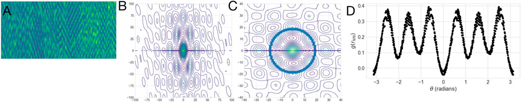
FIGURE 14. (A) Example kymograph showing moderate hexagonal ordering. (B) Two-dimensional autocorrelation of (A), with the central region used to determine the peak widths highlighted. (C) 2D autocorrelation with vertical distances rescaled so that the central peak is circularly symmetric. The ring represents points whose distance from the origin is equal to the expected average inter-particle spacing. (D) Intensity as a function of angle for the ring of points identified in (C), resulting in a C6 with magnitude 0.36 and angle 0.03 radians.
Using the measured width Δy, we can rescale the flow direction to produce a symmetric
Boundary stress microscopy. BSM measurements (Figure 9 were performed as described in [32, 35], but employing elastic films of relatively high modulus (G ∼ 1 MPa) to minimize possible effects of boundary compliance. Briefly, elastic films thickness 50 ± 3 μm were deposited by spin coating PDMS (Sylgard 184; Dow Corning) and a curing agent on 40 mm diameter glass cover slides (Fisher Sci) that were cleaned thoroughly by plasma cleaning and rinsing with ethanol and deionized water [35]. After deposition of PDMS, the slides were cured at 85 °C for 2 h. After curing, the PDMS was functionalized with 3-aminopropyl triethoxysilane (Fisher Sci) using vapor deposition for 40 min. Carboxylate-modified fluorescent spherical beads of radius 0.5 μm with excitation/emission at 520/560 nm were attached to the PDMS surface. Before attaching the beads to functionalized PDMS, the beads were suspended in a solution containing PBS solution (Thermo-Fisher). The concentration of beads used was 0.006% solids. The surface stresses at the interface were calculated using an extended traction force technique and codes given in Ref. [48]. Taking the component of the surface stress in the flow (velocity) direction, we obtain the scalar field
Data availability statement
The original contributions presented in the study are included in the article/Supplementary Material, further inquiries can be directed to the corresponding author.
Author contributions
JM, DB, and JU designed research; JM performed research; JM, DB, and JU analyzed data; and JM, DB, and JU wrote the paper.
Funding
This work was supported by the National Science Foundation (NSF) under Grant No. DMR-1809890. JU is supported, in part, by the Georgetown Interdisciplinary Chair in Science Fund.
Acknowledgments
The authors thank Peter Olmsted and Emanuela Del Gado for helpful discussions.
Conflict of interest
The authors declare that the research was conducted in the absence of any commercial or financial relationships that could be construed as a potential conflict of interest.
Publisher’s note
All claims expressed in this article are solely those of the authors and do not necessarily represent those of their affiliated organizations, or those of the publisher, the editors and the reviewers. Any product that may be evaluated in this article, or claim that may be made by its manufacturer, is not guaranteed or endorsed by the publisher.
Supplementary material
The Supplementary Material for this article can be found online at: https://www.frontiersin.org/articles/10.3389/fphy.2022.991540/full#supplementary-material
References
1. Vermant J, Solomon MJ. Flow-induced structure in colloidal suspensions. J Phys : Condens Matter (2005) 17:R187–216. doi:10.1088/0953-8984/17/4/r02
2. Morris JF. A review of microstructure in concentrated suspensions and its implications for rheology and bulk flow. Rheol Acta (2009) 48:909–23. doi:10.1007/s00397-009-0352-1
3. Lettinga MP. Fluids, colloids and soft materials: An introduction to. Soft Matter Phys (2016) 2016:81–110. doi:10.1002/9781119220510.ch6
4. Chen LB, Zukoski CF, Ackerson BJ, Hanley HJM, Straty GC, Barker J, et al. Structural changes and orientaional order in a sheared colloidal suspension. Phys Rev Lett (1992) 69:688–91. doi:10.1103/physrevlett.69.688
5. Holmqvist P, Lettinga MP, Buitenhuis J, Dhont JKG. Crystallization kinetics of colloidal spheres under stationary shear flow. Langmuir (2005) 21:10976–82. doi:10.1021/la051490h
6. Wu YL, Derks D, Blaaderen A, Imhof A. Melting and crystallization of colloidal hard-sphere suspensions under shear. Proc Natl Acad Sci U S A (2009) 106:10564–9. doi:10.1073/pnas.0812519106
7. Derks D, Wu YL, Blaaderen AV, Imhof A. Dynamics of colloidal crystals in shear flow. Soft Matter (2009) 5:1060–5. doi:10.1039/b816026k
8. Richard D, Speck T. The role of shear in crystallization kinetics: From suppression to enhancement. Sci Rep (2015) 5:14610. doi:10.1038/srep14610
9. Shereda LT, Larson RG, Solomon MJ. Boundary-driven colloidal crystallization in simple shear flow. Phys Rev Lett (2010) 105:228302. doi:10.1103/physrevlett.105.228302
10. Cheng X, Xu X, Rice SA, Dinner AR, Cohen I. Assembly of vorticity-aligned hard-sphere colloidal strings in a simple shear flow. Proc Natl Acad Sci U S A (2012) 109:63–7. doi:10.1073/pnas.1118197108
11. Xu X, Rice SA, Dinner AR. Influence of interlayer exchanges on vorticity-aligned colloidal string assembly in a simple shear flow. J Phys Chem Lett (2013) 4:3310–5. doi:10.1021/jz401722j
12. Mackay FE, Pastor K, Karttunen M, Denniston C. Modeling the behavior of confined colloidal particles under shear flow. Soft Matter (2014) 10:8724–30. doi:10.1039/c4sm01812e
13. Villada-Balbuena A, Jung G, Zuccolotto-Bernez AB, Franosch T, Egelhaaf SU. Layering and packing in confined colloidal suspensions. Soft Matter (2022) 18:4699–714. doi:10.1039/d2sm00412g
14. Kulkarni SD, Morris JF. Ordering transition and structural evolution under shear in Brownian suspensions. J Rheology (2009) 53:417–39. doi:10.1122/1.3073754
15. Pieper S, Schmid HJ. Layer-formation of non-colloidal suspensions in a parallel plate rheometer under steady shear. J Non-Newtonian Fluid Mech (2016) 234:1–7. doi:10.1016/j.jnnfm.2016.04.004
16. Küçüksönmez E, Servantie J. Shear thinning and thickening in dispersions of spherical nanoparticles. Phys Rev E (2020) 102:012604. doi:10.1103/physreve.102.012604
17. Myung JS, Song S, Ahn KH. Dynamics of model-stabilized colloidal suspensions in confined Couette flow. J Non-Newtonian Fluid Mech (2013) 199:29–36. doi:10.1016/j.jnnfm.2013.06.004
18. Morris JF. Shear thickening of concentrated suspensions: Recent developments and relation to other phenomena. Annu Rev Fluid Mech (2020) 52:121–44. doi:10.1146/annurev-fluid-010816-060128
19. Lee J, Jiang Z, Wang J, Sandy AR, Narayanan S, Lin XM. Unraveling the role of order-to-disorder transition in shear thickening suspensions. Phys Rev Lett (2018) 120:028002. Not sure what this means. doi:10.1103/PhysRevLett.120.028002
20. Goyal A, Gado ED, Jones SZ, Martys NS. Ordered domains in sheared dense suspensions: The link to viscosity and the disruptive effect of friction. J Rheology (2022) 66:1055–65. doi:10.1122/8.0000453
21. Boersma WH, Baets PJM, Laven J, Stein HN. Time-dependent behavior and wall slip in concentrated shear thickening dispersions. J Rheology (1991) 35:1093–120. doi:10.1122/1.550167
22. Lootens D, Damme H, Hébraud P. Giant stress fluctuations at the jamming transition. Phys Rev Lett (2003) 90:178301. doi:10.1103/PhysRevLett.90.178301
23. Nakanishi H, Si N, Mitarai N. Fluid dynamics of dilatant fluids. Phys Rev E (2012) 85:011401. doi:10.1103/PhysRevE.85.011401
24. Guy BM, Hermes M, Poon WCK. Towards a unified description of the rheology of hard-particle suspensions. Phys Rev Lett (2015) 115:088304. doi:10.1103/physrevlett.115.088304
25. Nagahiro SI, Nakanishi H. Negative pressure in shear thickening band of a dilatant fluid. Phys Rev E (2016) 94:062614. doi:10.1103/PhysRevE.94.062614
26. Hermes M, Guy BM, Poon WCK, Poy G, Cates ME, Wyart M. Unsteady flow and particle migration in dense, non-Brownian suspensions. J Rheology (2016) 60:905–16. doi:10.1122/1.4953814
27. Saint-Michel B, Gibaud T, Manneville S. Uncovering instabilities in the spatiotemporal dynamics of a shear-thickening cornstarch suspension. Phys Rev X (2018) 8:031006. doi:10.1103/PhysRevX.8.031006
28. Ovarlez G, Le AVN, Smit WJ, Fall A, Mari R, Chatté G, et al. Density waves in shear-thickening suspensions. Sci Adv (2020) 6:eaay5589. doi:10.1126/sciadv.aay5589
29. Gauthier A, Pruvost M, Gamache O, Colin A. A new pressure sensor array for normal stress measurement in complex fluids. J Rheology (2021) 65:583–94. doi:10.1122/8.0000249
30. Maharjan R, O’Reilly E, Postiglione T, Klimenko N, Brown E. Relation between dilation and stress fluctuations in discontinuous shear thickening suspensions. Phys Rev E (2021) 103:012603. doi:10.1103/physreve.103.012603
31. Rathee V, Blair DL, Urbach JS. Dynamics and memory of boundary stresses in discontinuous shear thickening suspensions during oscillatory shear. Soft Matter (2020) 17:1337–45. doi:10.1039/d0sm01917h
32. Rathee V, Blair DL, Urbach JS. Localized transient jamming in discontinuous shear thickening. J Rheology (2020) 64:299–308. doi:10.1122/1.5145111
33. Rathee V, Arora S, Blair DL, Urbach JS, Sood AK, Ganapathy R. Role of particle orientational order during shear thickening in suspensions of colloidal rods. Phys Rev E (2020) 101:040601. doi:10.1103/physreve.101.040601
34. Rathee V, Miller J, Blair DL, Urbach JS. Localized stress fluctuations drive shear thickening in dense suspensions. Proc Natl Acad Sci U S A (2022) 114:8740–5. doi:10.1073/pnas.1703871114
35. Dutta SK, Mbi A, Arevalo RC, Blair DL. Development of a confocal rheometer for soft and biological materials. Rev Sci Instrum (2013) 84:063702. doi:10.1063/1.4810015
36. Besseling R, Isa L, Weeks ER, Poon WC. Quantitative imaging of colloidal flows. Adv Colloid Interf Sci (2009) 146:1–17. doi:10.1016/j.cis.2008.09.008
37. Taylor GI. The spectrum of turbulence. Proc R Soc Lond A (1938) 164:476–90. doi:10.1098/rspa.1938.0032
38. He G, Jin G, Yang Y. Space-time correlations and dynamic coupling in turbulent flows. Annu Rev Fluid Mech (2017) 49:51–70. doi:10.1146/annurev-fluid-010816-060309
39. Koynov K, Butt HJ. Fluorescence correlation spectroscopy in colloid and interface science. Curr Opin Colloid Interf Sci (2012) 17:377–87. doi:10.1016/j.cocis.2012.09.003
40. Dong C, Ren J. Coupling of fluorescence correlation spectroscopy with capillary and microchannel analytical systems and its applications. ELECTROPHORESIS (2014) 35:2267–78. doi:10.1002/elps.201300648
41. Kunst BH, Schots A, Visser AJWG. Detection of flowing fluorescent particles in a microcapillary using fluorescence correlation spectroscopy. Anal Chem (2002) 74:5350–7. doi:10.1021/ac0256742
42. Gösch M, Blom H, Holm J, Heino T, Rigler R. Hydrodynamic flow profiling in microchannel structures by single molecule fluorescence correlation spectroscopy. Anal Chem (2000) 72:3260–5. doi:10.1021/ac991448p
43. Pan X, Yu H, Shi X, Korzh V, Wohland T. Characterization of flow direction in microchannels and zebrafish blood vessels by scanning fluorescence correlation spectroscopy. J Biomed Opt (2007) 12:014034. doi:10.1117/1.2435173
44. Pan X, Shi X, Korzh V, Yu H, Wohland T. Line scan fluorescence correlation spectroscopy for three-dimensional microfluidic flow velocity measurements. J Biomed Opt (2009) 14:024049. doi:10.1117/1.3094947
45. Ackerson BJ. Shear induced order and shear processing of model hard sphere suspensions. J Rheology (1990) 34:553–90. doi:10.1122/1.550096
46. Meer D. Impact on granular beds. Annu Rev Fluid Mech (2016) 49:463–84. doi:10.1146/annurev-fluid-010816-060213
47. O’Neill RE, Royer JR, Poon WCK. Liquid migration in shear thickening suspensions flowing through constrictions. Phys Rev Lett (2019) 123:128002. doi:10.1103/physrevlett.123.128002
Keywords: shear flow, rheology, colloids, shear thickening, order-disorder, phase transition
Citation: Miller JM, Blair DL and Urbach JS (2022) Order and density fluctuations near the boundary in sheared dense suspensions. Front. Phys. 10:991540. doi: 10.3389/fphy.2022.991540
Received: 11 July 2022; Accepted: 07 November 2022;
Published: 18 November 2022.
Edited by:
Luca Cipelletti, Université de Montpellier, FranceReviewed by:
Gabriel A. Caballero-Robledo, Unidad Monterrey, MexicoStefano Aime, École Supérieure de Physique et de Chimie Industrielles de la Ville de Paris, France
Copyright © 2022 Miller, Blair and Urbach. This is an open-access article distributed under the terms of the Creative Commons Attribution License (CC BY). The use, distribution or reproduction in other forums is permitted, provided the original author(s) and the copyright owner(s) are credited and that the original publication in this journal is cited, in accordance with accepted academic practice. No use, distribution or reproduction is permitted which does not comply with these terms.
*Correspondence: Jeffrey S. Urbach, urbachj@georgetown.edu