Simulating the Euler equations on multiple GPUs using Python

GPUs have become a household name in High Performance Computing (HPC) systems over the last 15 years. However, programming GPUs is still largely a manual and arduous task, which requires expert knowledge of the physics, mathematics, and computer science involved. Even though there have been large advances in automatic parallelization and GPU execution of serial code, it is still difficult to fully utilize the GPU hardware with such approaches. Many core numeric GPU codes are therefore still mostly written using low level C/C++ or Fortran for the host code. Several studies have shown that using higher level languages, such as Python, can make software development faster and with fewer bugs. We have developed a simulator based on PyCUDA and mpi4py in Python for solving the Euler equations on Cartesian grids. Our framework utilizes the GPU, and can automatically run on clusters using MPI as well as on shared-memory systems. Our framework allows the programmer to implement low-level details in CUDA C/C++, which is important to achieve peak performance, whilst still benefiting from the productivity of Python. We show that our framework achieves good weak and strong scaling. Our weak scaling achieves more than 94% efficiency on a shared-memory GPU system and more than 90% efficiency on a distributed-memory GPU system, and our strong scaling is close to perfect on both shared-memory and distributed-memory GPU systems.

1 Introduction

GPU computing started with proof-of-concept codes in the 1990s [1], continued with dedicated programming languages and platforms in the 2000s [2–5], and is now becoming a necessity within High Performance Computing (HPC). Most of the top level HPC systems in the world¹ are currently equipped with a large GPU partition that applications need to utilize efficiently in order to get resource allocations on the systems. The most common way of efficiently utilizing GPU devices has been to write specialized kernels in Nvidia CUDA C++ for the “inner loops”, and calling these kernels from a C/C++ or Fortran host application through an API.

Although most existing HPC codes are written in C/C++ and Fortran, a growing portion of scientific software is developed in Python, which is currently one of the most popular programming languages for scientific computing applications [6]. Within STEM education and training, Python is also a popular choice, leading to a new generation of scientific programmers and researchers which is more proficient in Python than the traditional compiled languages. For experimentation and prototyping, Python is of particular interest due to its low verbose code and high productivity [7, 8], how it can be combined with C++ and Fortran code, and the wide range of available tools and third-party libraries for numerical and scientific applications².

Holm, Brodtkorb and Sætra [9] investigated GPU computing with Python for single-GPU systems, and found that the overhead of using Python for stencil-based simulator codes, compared to low-level languages, is negligible with regards to performance. The energy efficiency does vary some between different numerical schemes, optimization levels and GPUs, but the run time is unsurprisingly the most important factor. They note that the productivity of working with Python is significantly higher than using C++. Herein, we take the first step to extend these findings to a multi-GPU setting. We show that Python code with GPU acceleration can be moved from the prototype stage into HPC production code, obtaining good results in terms of parallel efficiency and scaling on two HPC systems with very different characteristics, also without architecture-specific optimization. Our code can be run through scripts for batch runs, but is also easily used interactively (in a read-eval-print manner) from Jupyter notebooks, also for multi-GPU simulation with MPI. We are simulating the Euler equations using finite-volume methods with a stencil-based high-resolution time-stepping scheme (Section 2.1 and references therein) for our experiments. The Euler equations describe adiabatic and inviscid flow, and have a wide range of applications, from numerical weather prediction to simulation of air flow around an aircraft wing. The methods we use may also be applied to other hyperbolic conservation and balance laws, and have been demonstrated to achieve high performance both on single GPUs [10, 11] and multiple GPUs [12] for the shallow-water equations and stencil-based solvers in general.

There exist other similar Python-based frameworks that utilize GPUs for computational fluid dynamics. Witherden, Farrington and Vincent [13] describes PyFR, a framework for solving the Euler and Navier-Stokes equations on unstructured grids using both CPUs and GPUs. The framework relies on a domain specific language to specify point-wise kernels that are interpreted at runtime and used to generate CUDA kernels that run on the GPUs. Walker and Niemeyer [14] apply the swept rule for solving the two-dimensional heat equation and Euler equations on heterogeneous architectures. They note that great care must be taken when designing a solver for such architectures in order to achieve decent speed-up. Oden [15] investigates the differences between native CUDA C++ code and CUDA code written in Python using Numba, using both microbenchmarks and real applications. She shows that the Numba versions only reach between 50% and 85% of the performance of the native CUDA C++ for compute-intensive benchmarks. This suggests that it is still necessary to “hand code” the inner loops in order to get maximum performance on the GPU.

The use of Python for scientific computing and machine learning has exploded over the last decade [16, 17]. For HPC applications, one major challenge is to balance productivity with efficiency. In the work presented here, the highest efficiency is always within reach since the numerical schemes are written in CUDA C++, allowing for fine-tuning the code to a particular GPU. At the same time, high productivity is facilitated by keeping all other parts of the code in Python. Moreover, by using only standard Python and well-known and mature third-party libraries, debugging and profiling of the code is kept manageable.

2 Materials and methods

This section details the mathematical discretization, its implementation on GPU and extension to multiple GPUs. We also outline how the profiling of the MPI + GPU application was performed.

2.1 Mathematical formulation

The two-dimensional Euler Equations are a simplification of the more complex Navier-Stokes equations, and can be written

${\left[\begin{array}{c}\hfill \rho \hfill \\ \hfill \rho u\hfill \\ \hfill \rho v\hfill \\ \hfill E\hfill \end{array}\right]}_t+{\left[\begin{array}{c}\hfill \rho u\hfill \\ \hfill \rho u^2+p\hfill \\ \hfill \rho vu\hfill \\ \hfill u\left(E+p\right)\hfill \end{array}\right]}_x+{\left[\begin{array}{c}\hfill \rho v\hfill \\ \hfill \rho uv\hfill \\ \hfill \rho v^2+p\hfill \\ \hfill v\left(E+p\right)\hfill \end{array}\right]}_y=\left[\begin{array}{c}\hfill 0\hfill \\ \hfill 0\hfill \\ \hfill 0\hfill \\ \hfill 0\hfill \end{array}\right],(1)$

in which ρ is the fluid density, the vector [ρu, ρv] represents the momentum, E is the total energy, and p is the pressure. The total energy can be written as

$E=\frac{1}{2}\rho \left(u^2+v^2\right)+p/\left(\gamma -1\right),(2)$

in which γ is the adiabatic exponent. We can also write the equations on vector form,

$\frac{\partial Q}{\partial t}+\frac{\partial F\left(Q\right)}{\partial x}+\frac{\partial G\left(Q\right)}{\partial y}=0,$

in which Q is our vector of conserved variables, and F and G are the source terms that govern the fluid dynamics. We can then discretize our spatial derivatives, and end up with the following ordinary differential equation that we have to solve in time:

$\frac{dQ}{dt}=-F_x\left(Q\right)-G_y\left(Q\right).(3)$

There are multiple ways of solving these equations. We can for example use the classical Lax-Friedrichs numerical scheme, which gives us the following discretization in two dimensions:

$\begin{array}{ll}\hfill Q_{i,j}^{n+1}& =\frac{1}{4}\left[Q_{i+1,j}^n+Q_{i-1,j}^n+Q_{i,j+1}^n+Q_{i,j-1}^n\right]\hfill \\ \hfill & -\frac{\mathrm{\Delta }t}{2\mathrm{\Delta }x}\left[F\left(Q_{i+1,j}^n\right)-F\left(Q_{i-1,j}^n\right)\right]\hfill \\ \hfill & -\frac{\mathrm{\Delta }t}{2\mathrm{\Delta }y}\left[G\left(Q_{i,j+1}^n\right)-G\left(Q_{i,j-1}^n\right)\right],\hfill \end{array}(4)$

with a time step restricted by a CFL condition. This scheme is a two-dimensional scheme, in which we compute the new solution based on a two-dimensional stencil.

It is well known that this classical first order scheme is numerically dissipative, leading to overly smeared solutions as time progresses. We can improve on this, by using a higher-order scheme. In this work, we have used a second-order accurate MUSCL-Hancock scheme [18, 19], which in one dimension can be written

${\bar{Q}}_i^L=Q_i^L+\frac{1}{2}\frac{\mathrm{\Delta }t}{\mathrm{\Delta }x}\left[F\left(Q_i^L\right)-F\left(Q_i^R\right)\right],(5)$

${\bar{Q}}_i^R=Q_i^R+\frac{1}{2}\frac{\mathrm{\Delta }t}{\mathrm{\Delta }x}\left[F\left(Q_i^L\right)-F\left(Q_i^R\right)\right].(6)$

Here, ${\bar{Q}}_i^L$ denotes the reconstructed value at the left hand side of cell i, and equivalently ${\bar{Q}}_i^R$ denotes the reconstructed value at the right hand side. This means that we have the two states, ${\bar{Q}}_i^R$ and ${\bar{Q}}_{i+1}^L$, at the interface between cells i and i + 1, and we use the Harten-Lax-van Leer (HLL) approximate Riemann solver [20, 21] with these two states to compute the HLL flux, ${\bar{F}}_{i+1/2}$, across the interface. The scheme is second-order accurate in one dimension [21]. To extend it to two-dimensional problems, we use a dimensional splitting scheme that is second-order accurate every other time step [21, 22],

$Q^{\ast }=Y^{\mathrm{\Delta }t}{X}^{\mathrm{\Delta }t}{Q}^n,(7)$

$Q^{n+2}=X^{\mathrm{\Delta }t}{Y}^{\mathrm{\Delta }t}{Q}^{\ast }.(8)$

Here, X^Δt and Y^Δt are the one-dimensional operators that advance the solution in time along the x and y-axis, respectively:

$X^{\mathrm{\Delta }t}=Q^n-\mathrm{\Delta }t\left[{\bar{F}}_{i+1/2,j}-{\bar{F}}_{i-1/2,j}\right],(9)$

$Y^{\mathrm{\Delta }t}=Q^n-\mathrm{\Delta }t\left[{\bar{G}}_{i,j+1/2}-{\bar{G}}_{i,j-1/2}\right].(10)$

The time step is restricted by a CFL condition, so that the maximum time step advects the solution at most one cell in the domain. The CFL condition can be written as

$\mathrm{\Delta }t\le C\text{min}\left(\frac{\mathrm{\Delta }x}{S_{\mathit{max}}^x},\frac{\mathrm{\Delta }y}{S_{\mathit{max}}^y}\right),(11)$

in which C is the CFL number, $S_{\mathit{max}}^x$ is the maximum wave speed present in the domain along the x-axis, and similar for the y-axis. A practical choice for approximating the time step is

$\mathrm{\Delta }t\le C\text{min}\left(\frac{\mathrm{\Delta }x}{|u|+c},\frac{\mathrm{\Delta }y}{|v|+c}\right)=C\text{min}\left(\frac{\mathrm{\Delta }x}{|\rho u/\rho |+\sqrt{\gamma \rho }},\frac{\mathrm{\Delta }y}{|\rho v/\rho |+\sqrt{\gamma \rho }}\right),(12)$

but it should be noted that this formulation must be used with caution, and may yield unstable simulations even with low CFL numbers (see, e.g. [21]).

2.2 Program structure

The simulator is written using Python (3.7.12), NumPy (1.21.6), netcdf4 (1.5.8), PyCUDA [23] (2021.1), mpi4py [17, 24, 25] (3.1.3), OpenMPI (4.1.0), and CUDA (11.4.1) to combine the power of multiple GPUs in a distributed-memory or shared-memory architecture. The traditional programming language for HPC has been Fortran—which is evident from the large array of Fortran programs running on supercomputers today. The common explanation for this is that nothing can surpass Fortran in terms of performance. Whilst it may be true that Fortran typically runs faster than Python, the approach of using Python has some merits [26]. We use Python here to combine traditional MPI-based supercomputing with GPU computing in a hybrid approach. The libraries we use have a base/core in C/C++, which gives us the flexibility of Python with close to the speed of compiled languages.

The program structure for a single-GPU simulation is shown in Figure 1. Simulator initialization constructs initial conditions, a CUDA context and a simulator ready for time-stepping. Initial conditions and all simulation parameters needed to re-run the simulation is saved to a NetCDF file for easy reproducible results. Each time step consists of enforcing the boundary conditions upon reading in data from the previous time step, evaluation of new fluxes and any right-hand side source terms, forward time integration, and an optional computation of the maximum time-step size (for the next time step) based on the CFL condition. If the maximum time-step size is not computed, a fixed time-step size must be provided. Intermediate results can be written to the NetCDF file at prescribed simulation times.

FIGURE 1

FIGURE 1. Program flow on a single GPU. All the boxes within the dotted square represent stages within the CUDA kernel. After completing all the CUDA kernel stages, the simulation is advanced one step in time. The dashed boxes are optional, and if the max time-step size if not computed, a fixed time-step size must be given.

2.3 CUDA implementation

The numerical scheme outlined in the Section 2.1 is implemented as a single-GPU kernel that computes either Eq. (7) or Eq. (8) depending on a flag sent as a variable. This means that after two kernel invocations, both equations are computed once and the solution is evolved two time steps (recall that the numerical scheme is only second-order accurate every second time step). The GPU is completely managed through PyCUDA: The device is controlled through the device API (pycuda.driver), the CUDA C++-kernels are compiled using just-in-time compilation (pycuda.compiler), and data is stored using GPU Arrays (pycuda.gpuarray.GPUArray). CUDA kernels are run using prepared function calls. If we examine the data dependencies of the numerical scheme (i.e., the numerical stencil), we observe that the kernel requires a two-row halo in all directions, as shown in Figure 2. The kernel is then implemented in a standard way, using shared memory on the GPU to store the physical and reconstructed variables. The principles from our earlier implementations of numerical schemes for shallow-water simulations [10, 11] are applied. By computing both in the x-dimension and the y-dimension for each kernel execution we avoid having to read the physical values twice, at the expense of an extra row and column of halo cells. In this work, we have used a fixed CUDA block size of 16 by 8 cells, but the code does contain an autotuner which can be used to optimize the block size for performance on a particular GPU (see Section 4.2 in [9]).

FIGURE 2

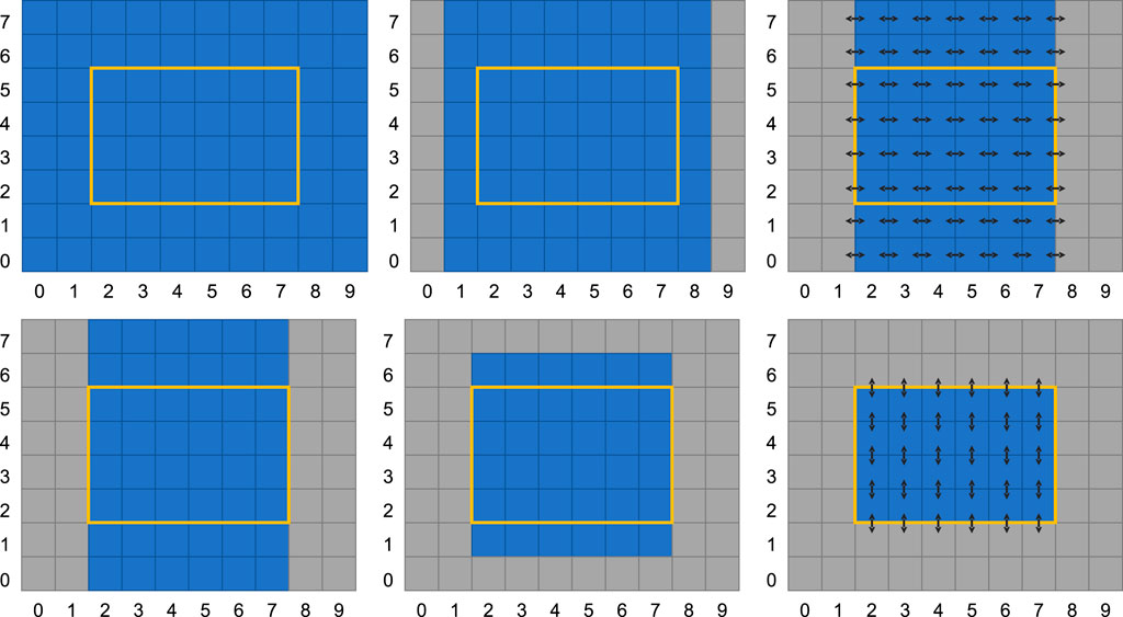
FIGURE 2. Halo region for the CUDA kernel when computing Eq. 8. The top row shows how the input values (left) are used to compute the slopes (center) along the x-axis. The slopes are consequently used to compute the face fluxes (right). Equivalently for the y-axis, the bottom row shows how the input values (left) are used to compute the slopes (center), and finally the fluxes along the y-axis. Thus, an input grid of 8 × 10 cells is used to compute the fluxes for the inner 4 × 6 cells.

In addition to the numerical scheme presented for the Euler equations, the simulator also contains various numerical schemes for solving the two-dimensional shallow-water equations.

2.4 Extension to multiple GPUs

For multi-GPU simulations we introduce Python classes for an MPI grid and an MPI simulator. Each MPI process has its own MPI simulator and CUDA context. The MPI grid handles domain decomposition and the necessary bookkeeping, keeping track of which subdomains that need to communicate and where the global boundaries are found. Both one- and two-dimensional domain decomposition are supported. In both cases the global Cartesian grid is decomposed uniformly between all MPI ranks, such that each subdomain will have at most two neighbors in 1D and at most four neighbors in 2D. The MPI simulator extends the base simulator class and adds the necessary functionality for exchanging halo cells between neighbouring subdomains and computing global Δt for simulations with a variable time-step size. All MPI calls are done through mpi4py.

In Figure 3, all the stages of a multi-GPU simulation are shown (from the perspective of one subdomain/MPI rank), divided between two CUDA streams. To minimize the communication overhead, we use asynchronous memory transfers that overlap with computations. This enables us to hide most of the cost associated with downloading, exchanging and uploading halo cells each time step. There are some prerequisites for this: Host memory needs to be pagelocked, the memory operations must be asynchronous and they must be issued on a different stream than the computational kernel(s) that is intended to run simultaneously. The issue order of computational kernels and memory operations on the two streams may impact the degree of overlap. Furthermore, the size of the computational domains and different hardware specifications (GPU generation and class) may also lead to a varying degree of overlapping execution between the two streams.

FIGURE 3

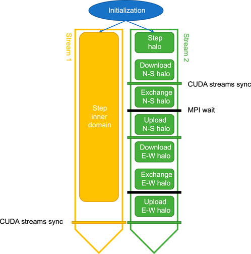
FIGURE 3. By using two CUDA streams we can perform memory operations and computations simultaneously. The inner domain is advanced one time step in Stream 1 and the halo in Stream 2. Since the inner domain usually is much bigger than the halo, the compute time spent on the inner domain in Stream 1 will mask the time used for exchanging halo regions with neighboring subdomains in Stream 2, including downloading (GPU to CPU), send/receive with MPI, and uploading (CPU to GPU). The step stage executes the same kernel for both streams, shown in Figure 1, but for different areas of the domain.

Figure 4 shows a schematic outline of the complete halo cell exchange performed in Stream 2, related to the computational grid. The halo cell buffers for all four boundaries of each subdomain is allocated through PyCUDA’s device interface. They are allocated once as pagelocked memory at simulation initialization, and then used throughout the rest of the simulation. These buffers are also used for the global boundaries for certain boundary conditions, e.g., periodical boundaries. Memory transfers are performed asynchronously by calling PyCUDA Memcpy2D objects, specifying the stream we want the memory operation issued to. The sizes of the halo regions are easy to adjust to permit the use of other numerical schemes with different stencil sizes.

FIGURE 4

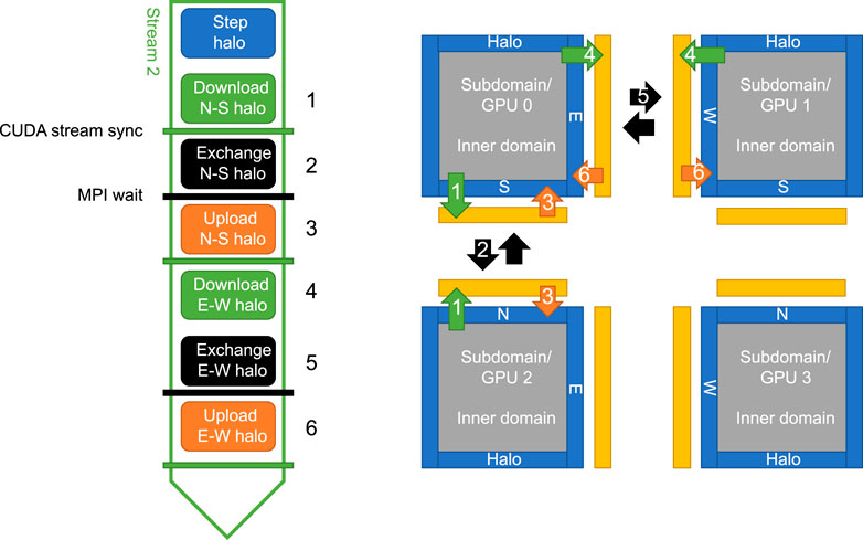
FIGURE 4. This schematic outline shows the different stages executed in Stream 2 and how they relate to the computational grid. Note that the halo computed in the first stage includes both the regions that will be copied to neighboring subdomains (inne halo) and the areas where values from neighboring subdomains will be copied into (outer halo).

The exchange of halo regions with neighboring subdomains is done with matching non-blocking MPI Isend/Irecv pairs with MPI wait at the global synchronization points. The corner cells are transferred first in the north-south direction, then in the east-west direction. This minimizes the size of the transfer buffers and avoids diagonal transfers between subdomains, at the expense of an extra MPI synchronization to ensure that all north-south exchanges are done before any east-west exchanges start. As the internal domain is being computed simultaneous to the full halo exchange process, including all but the final synchronization point, this effectively hides most of the communication overhead.

2.5 Profiling multi-GPU applications

For a complete documentation of the tools used herein, we refer to the user guides. The walk-through given here describes our use of the tools and may also serve as a quickstart guide for others.

The Nvidia Visual Profiler and the nvprof command line interface (CLI) tool have long been the go-to profiling and analysis tools for GPU applications, the latter for remote profiling on servers. In 2018, Nvidia introduced a new suite of Nsight Tools; Systems³, Compute, and Graphics, which is now the new standard profiling tools. Nsight Systems (nsys) for complete system profiling and analysis, including OpenGL, OpenMP, MPI, and CPU sampling; Nsight Compute (ncu) for GPU kernel profiling and analysis; and Nsight Graphics (ngfx) for profiling graphics applications.

This is how we profiled our code with Nsight Systems on the remote systems (using CLI):

1) Install Nsight Systems (x86_64, IBM Power, and ARM SDSA target versions are available in the CUDA Toolkit)

2) Run nsys profile <application executable>

3) To trace MPI, add the -t option. Here we are tracing CUDA, NVTX, OS runtime and MPI: -t cuda,nvtx,osrt,mpi

4) Copy or move report1.qdrep (standard name) to local machine

5) Open report1.qdrep with nsys-ui to view profile

It is also possible to do live profiling of a remote host by connecting your locally running Nsight Systems UI to a daemon running on the remote system, but this is generally not recommended due to security issues with unencrypted connection and plain-text password storage.

3 Results

The simulator has been profiled using Nsight Systems for multi-GPU and MPI performance. Furthermore, the simulator has been benchmarked on two systems, by instrumenting the Python code to measure run times, demonstrating good weak and strong scaling. We describe the experiment setup in terms of simulation case and hardware, and present the results.

3.1 Experiment description

We have simulated the Kelvin-Helmholtz instability, which models the dynamics occurring at the interface between two fluids with different speeds. An example of such a simulation is shown in Figure 5. This phenomenon occurs naturally, e.g., in a stratified atmosphere when there is a layer of fast moving air over a slower moving layer of air.

FIGURE 5

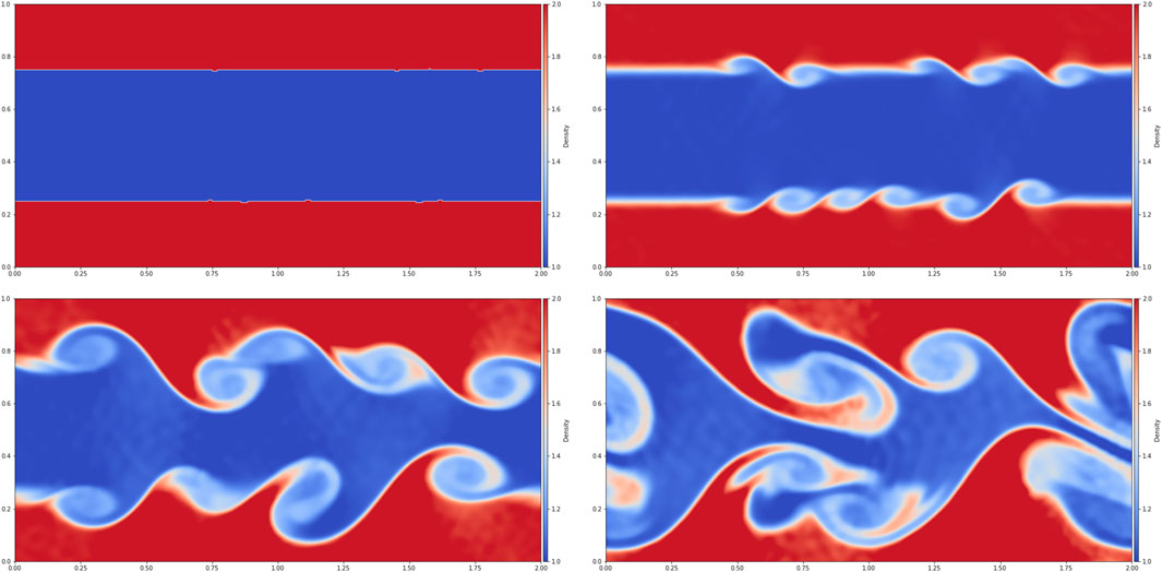
FIGURE 5. A simulation of the Kelvin-Helmholtz instability. The four panels show density in the initial conditions and after 1, 2 and 3 s of simulation time. See animation at https://www.youtube.com/watch?v=ejCzlwIT--w.

We generate a periodic test case in which both the upper and lower quarter of the fluid move towards the left, whilst the center moves towards the right. We define the two regions with the following properties:

${\rho }_1=1.0,u_1=0.5,v_1=0,(13)$

$\begin{array}{l}\hfill \text{and}\\ \hfill {\rho }_2=2.0,u_2& =-0.5,v_2=0.\hfill \end{array}(14)$

The total energy is computed using Eq. (2), in which we set the adiabatic exponent γ = 1.4. The interface between the two regions is slightly perturbed to trigger the instability.

3.2 Benchmark systems

The scaling benchmark has been run on two different systems with very different characteristics, but on both systems the Slurm Workload Manager was used to launch all jobs.

The first system, the DGX-2⁴, is a shared-memory architecture with 16 Nvidia Tesla V100 GPUs. All the GPUs have 32 GB of local memory each (total of 512 GB) and share 1.5 TB main memory. The peak performance in double precision is 125 teraflops. We had exclusive access to this system while running the experiments.

The second system, Saga⁵, is a distributed-memory system and a part of the Norwegian research infrastructure. The system has eight nodes with four Nvidia Tesla P100 GPUs installed in each node. The GPUs have 16 GB of local memory each. Each node has two CPUs with 24 cores and 384 GiB memory each. The nodes are connected by InfiniBand HDR. This system was shared with other users while running the experiments.

3.3 Multi-GPU profiling

From Figure 6 we see that the memory operations (downloading from, and uploading to, the GPU) and MPI communication and synchronization with other subdomains are performed simultaneously with the execution of the computational kernel for the inner domain. As the domain size is increased, so is the ratio of the inner domain area to the halo area. Thus, at some point, the compute time for the inner domain will hide all the cost of halo cell exchange process except the API calls and other fixed overheads. Since there are four conserved variables (Eq. 1) and up to four neighboring subdomains (Figure 4), this results in a total of 16 sets of downloading, uploading and exchanging halo cell buffers for the subdomains which are not on the global domain boundary.

FIGURE 6

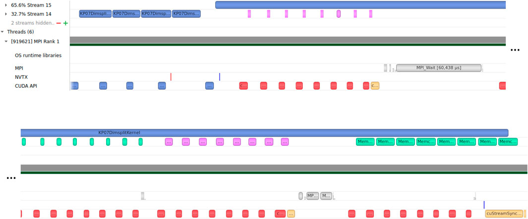
FIGURE 6. Screendump of timeline in the Nsight Systems UI zoomed in on one time step on one GPU (in a two-GPU simulation), showing overlap of memory operations (in Stream 14) and MPI communication (designated MPI), and the computational kernel for the inner domain (in Stream 15). The CUDA API calls are shown in the bottom row. Note that the timeline is split over two rows. The color codes for the bars are as follows: Blue is compute kernel execution or API call, purple is download (GPU to CPU), green is upload (CPU to GPU), gray is MPI Isend/Irecv or wait, red is memory API calls, and yellow is CUDA thread synchronization.

3.4 Multi-GPU scaling

For all scaling experiments, the domain size is set such that close to all available memory is used on each GPU, and we run the simulation for 200 time steps with a fixed time-step size. For weak scaling the subdomain size per GPU is kept fixed, and we run experiments using from one GPU up to the available number GPUs in the system. For strong scaling the global domain size is fixed, and we run experiments using from four GPUs (the domain size is scaled to fit on four GPUs) up to the available number of GPUs in the system. All initialization, writing of results to NetCDF files and cleanup after the last time step are not included in the time measurements, meaning that we measure only the stages of Stream 1 and Stream 2 shown in Figure 3.

Results from scaling experiments on the DGX-2 system is shown in Figure 7. For weak scaling, shown in the panel to the left, we have a minimum efficiency of 94% compared to the single-GPU run. There are some variations in the efficiency in the interval between 94% and 96% efficiency from 9 to 16 GPUs. This suggests that there are still some overheads connected to the halo cell exchange that are not completely hidden. For strong scaling, shown in the panel to the right, we observe linear scaling from 4 to 16 GPUs, meaning that no significant extra cost in terms of run time is incurred when going from 4 to 16 GPUs.

FIGURE 7

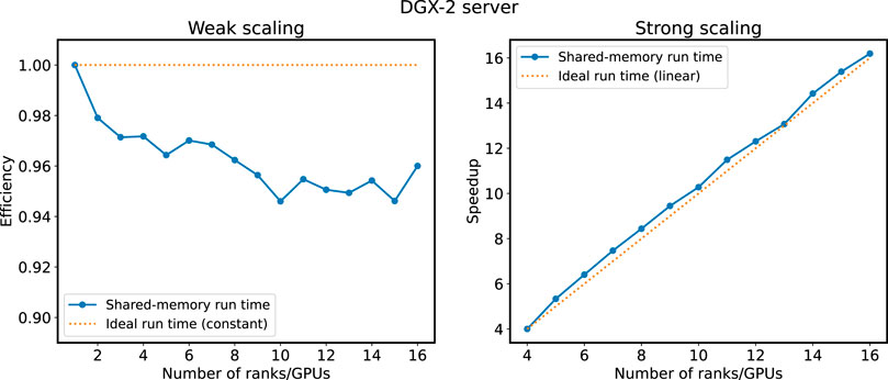
FIGURE 7. Results from scaling experiments on DGX-2 shared-memory system. Weak scaling (1–16 GPUs) is shown in the left panel and strong scaling (4–16 GPUs) is shown in the right panel. Run times are normalized with respect to the single rank/GPU experiment for weak scaling and the four ranks/GPUs experiment for strong scaling.

Results from scaling experiments on the Saga cluster is shown in Figure 8. There are two graphs for weak scaling, shown in the panel to the left, one for shared memory on a single node and one for distributed memory on 1–4 nodes with one GPU on each node. In both graphs, measurements are normalized with respect to the single-node single-GPU run time. The single-node weak scaling have a minimum efficiency of 98% and the multi-node weak scaling have a minimum efficiency of 90%. Again, this shows that there is still some overheads connected to the halo cell exchange that is not completely hidden. We attribute the lower efficiency in Saga (for the distributed-memory run times), compared to the shared-memory run times, to the interconnect and the fact that this is a shared system with many active users. We would have liked to use up to 16 GPUs for the weak scaling experiments, but limitations due to congestion and Slurm setup made this difficult. Strong scaling, shown in the panel to the right, scales linearly from 4 to 16 GPUs.

FIGURE 8

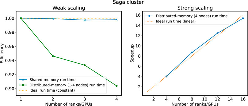
FIGURE 8. Results from scaling experiments on the Saga cluster. Weak scaling (1–4 GPUs on a single node and 1–4 nodes with one GPU on each node) is shown in the left panel and strong scaling (4–16 GPUs divided equally between four nodes) is shown in the right panel. Run times are normalized with respect to the single rank/GPU experiment for weak scaling and the four ranks/GPUs experiment for strong scaling.

4 Discussion

We have described a Python-CUDA C++-based prototype framework for multi-GPU simulation of the Euler equations using finite-volume methods. By implementing everything but the numerical schemes in Python, the code is kept short and manageable, which facilitates productivity. No domain specific language has been used and only a limited number of well-known and mature third-party libraries. This enhances the readability of exception stack traces and reduces the vulnerability of discontinued third-party libraries for GPU acceleration, inter-process communication, domain decomposition, etc. The numerical scheme is implemented in CUDA C++, which gives a high level of flexibility and the possibility to optimize for a particular GPU. Autotuning of CUDA block size is implemented and can give increased performance portability between different generations and classes of GPUs. The code can be adapted to simulate other conservation laws and to use different numerical schemes. The simulator has been shown to be efficient through profiling and scalability experiments on both shared-memory and distributed-memory systems. As the amount of scientific Python code bases grows together with the number of GPU-accelerated HPC-systems, these are promising results.

The results show that there are still improvements to be made, particularly for distributed-memory systems without a fast interconnect. One possible option is to use ghost cell expansion [12, 27], which would increase the size of the halo cell regions, allowing for running multiple time steps for each halo cell exchange. Hybrid MPI + OpenMP (threads) would decrease the number of total MPI messages, but since inter-process communication costs already are efficiently hidden by overlapping with computation on the shared-memory system, this seems like a high investment in code complexity for a low return in terms of reduced run time. So-called MPI + MPI (MPI-integrated shared memory) and experimentation with processor affinity are also something to be explored.

Future work includes adding more applications and numerical schemes, with extension to three dimensions. A more robust implementation of asynchronous communication that take GPU (PCIe, NVLink and NVSwitch) and system interconnect into account could further increase the scaling performance by leveraging CUDA-aware MPI, UCX, and RDMA [28, 29]. Domain decomposition for load balancing in heterogeneous systems (CPUs and GPUs, or different generations and classes of GPUs) would allow for better performance portability for simulations on heterogeneous systems and multi-GPU simulations. The scaling benchmark should also be run on larger systems to investigate the limits of scalability and how the workload manager’s resource allocation and management may affect the performance, depending on which flags that are used. Comparison studies on alternatives to CUDA C++ would give more insight into efficiency-productivity considerations, including HIP (by using HIPIFY), SYCL and even pragma/directive-based approaches. This would also break the current dependency on Nvidia GPUs.

The code is available at https://github.com/babrodtk/ShallowWaterGPU.

Data availability statement

Publicly available datasets were analyzed in this study. This data can be found here: https://github.com/babrodtk/ShallowWaterGPU.

Author contributions

AB—conceptualization; methodology; software; writing—original draft; writing—review and editing; visualization; funding acquisition. MS—conceptualization; software; validation; investigation; writing—original draft; writing—review and editing; visualization; funding acquisition.

Funding

The research contribution of MS is funded by The Norwegian Research Council under the project “HAVVARSEL—Personalized ocean forecasts in a two-way data flow system” (310515). The shared-memory simulations were performed on a system provided by Simula Research Laboratory under the eX3 project⁶. The Saga cluster simulations were performed on resources provided by Sigma2—the National Infrastructure for High Performance Computing and Data Storage in Norway under project number nn9882k.

Conflict of interest

The authors declare that the research was conducted in the absence of any commercial or financial relationships that could be construed as a potential conflict of interest.

Publisher’s note

All claims expressed in this article are solely those of the authors and do not necessarily represent those of their affiliated organizations, or those of the publisher, the editors and the reviewers. Any product that may be evaluated in this article, or claim that may be made by its manufacturer, is not guaranteed or endorsed by the publisher.

Footnotes

¹https://eurohpc-ju.europa.eu/about/our-supercomputers, https://www.olcf.ornl.gov/frontier/, and https://www.top500.org/.

²https://numfocus.org/sponsored-projects/affiliated-projects and https://numfocus.org/sponsored-projects.

³https://docs.nvidia.com/nsight-systems/UserGuide/index.html.

⁴https://www.ex3.simula.no/resources.

⁵https://documentation.sigma2.no/hpc_machines/saga.html.

⁶https://www.ex3.simula.no/.

References

1. Larsen E, McAllister D. Fast matrix multiplies using graphics hardware. In: ACM/IEEE Conference on Supercomputing. New York, NY, USA: ACM (2001). p. 55.

CrossRef Full Text | Google Scholar

2. Owens JD, Luebke D, Govindaraju N, Harris M, Krüger J, Lefohn AE, et al. A survey of general-purpose computation on graphics hardware. Computer Graphics Forum (2007) 26:80–113. doi:10.1111/j.1467-8659.2007.01012.x

CrossRef Full Text | Google Scholar

3. Owens J, Houston M, Luebke D, Green S, Stone J, Phillips J. GPU computing. Proc IEEE (2008) 96:879–99. doi:10.1109/JPROC.2008.917757

CrossRef Full Text | Google Scholar

4. Brodtkorb AR, Dyken C, Hagen TR, Hjelmervik JM, Storaasli OO. State-of-the-art in heterogeneous computing. Scientific Programming (2010) 18:1–33. doi:10.3233/SPR-2009-0296

CrossRef Full Text | Google Scholar

5. Brodtkorb AR, Hagen TR, Sætra ML. Graphics processing unit (GPU) programming strategies and trends in GPU computing. J Parallel Distributed Comput (2013) 73:4–13. doi:10.1016/j.jpdc.2012.04.003

CrossRef Full Text | Google Scholar

6. Barba LA. The Python/jupyter ecosystem: Today’s problem-solving environment for computational science. Comput Sci Eng (2021) 23:5–9. doi:10.1109/MCSE.2021.3074693

CrossRef Full Text | Google Scholar

7. Nanz S, Furia CA. A comparative study of programming languages in rosetta code. In: 2015 IEEE/ACM 37th IEEE International Conference on Software Engineering, 1 (2015). p. 778–88. doi:10.1109/ICSE.2015.90

CrossRef Full Text | Google Scholar

8. Prechelt L. An empirical comparison of seven programming languages. Comput J (2000) 33(10):23–9. doi:10.1109/2.876288

CrossRef Full Text | Google Scholar

9. Holm HH, Brodtkorb AR, Sætra ML. GPU computing with Python: Performance, energy efficiency and usability. Computation (2020) 8:4. doi:10.3390/computation8010004

CrossRef Full Text | Google Scholar

10. Brodtkorb AR, Sætra ML, Altinakar M. Efficient shallow water simulations on GPUs: Implementation, visualization, verification, and validation. Comput Fluids (2012) 55:1–12. doi:10.1016/j.compfluid.2011.10.012

CrossRef Full Text | Google Scholar

11. Brodtkorb AR, Sætra ML. Explicit shallow water simulations on GPUs: Guidelines and best practices. CMWR (2012).XIX international conference on water resources.

Google Scholar

12. Sætra M, Brodtkorb A. Shallow water simulations on multiple GPUs. In: Jónasson K, editor. Applied parallel and scientific computing. Springer Berlin/Heidelberg (2012).

Google Scholar

13. Witherden FD, Farrington AM, Vincent PE. PyFR: An open source framework for solving advection–diffusion type problems on streaming architectures using the flux reconstruction approach. Computer Phys Commun (2014) 185:3028–40. doi:10.1016/j.cpc.2014.07.011

CrossRef Full Text | Google Scholar

14. Walker AS, Niemeyer KE. Applying the swept rule for solving two-dimensional partial differential equations on heterogeneous architectures. Math Comput Appl (2021) 26:52. doi:10.3390/mca26030052

CrossRef Full Text | Google Scholar

15. Oden L. Lessons learned from comparing C-CUDA and Python-Numba for GPU-Computing. In: 2020 28th Euromicro International Conference on Parallel, Distributed and Network-Based Processing. PDP (2020).

CrossRef Full Text | Google Scholar

16. Barba LA, Klöckner A, Ramachandran P, Thomas R. Scientific computing with Python on high-performance heterogeneous systems. Comput Sci Eng (2021) 23:5–7. doi:10.1109/MCSE.2021.3088549

CrossRef Full Text | Google Scholar

17. Fink Z, Liu S, Choi J, Diener M, Kale LV. Performance evaluation of Python parallel programming models: Charm4Py and mpi4py. In 2021 IEEE/ACM 6th International Workshop on Extreme Scale Programming Models and Middleware (ESPM2) (2021).

CrossRef Full Text | Google Scholar

18. van Leer B. Towards the ultimate conservative difference scheme. V. A second-order sequel to Godunov’s method. J Comput Phys (1979) 32:101–36. doi:10.1016/0021-9991(79)90145-1

CrossRef Full Text | Google Scholar

19. van Leer B. On the relation between the upwind-differencing schemes of godunov, engquist–osher and roe. SIAM J Scientific Stat Comput (1984) 5:1–20. doi:10.1137/0905001

CrossRef Full Text | Google Scholar

20. Harten A, Lax PD, van Leer B. On upstream differencing and godunov-type schemes for hyperbolic conservation laws. SIAM Rev (1983) 25:35–61. doi:10.1137/1025002

CrossRef Full Text | Google Scholar

21. Toro E. Riemann solvers and numerical methods for fluid dynamics: A practical introduction. Heidelberg: Springer Berlin Heidelberg (2013).

Google Scholar

22. Warming RF, Beam RM. Upwind second-order difference schemes and applications in aerodynamic flows. AIAA J (1976) 14:1241–9. doi:10.2514/3.61457

CrossRef Full Text | Google Scholar

23. Klöckner A, Pinto N, Lee Y, Catanzaro B, Ivanov P, Fasih A. PyCUDA and PyOpenCL: A scripting-based approach to GPU run-time code generation. Parallel Comput (2012) 38:157–74. doi:10.1016/j.parco.2011.09.001

CrossRef Full Text | Google Scholar

24. Dalcín L, Paz R, Storti M. MPI for Python. J Parallel Distributed Comput (2005) 65:1108–15. doi:10.1016/j.jpdc.2005.03.010

CrossRef Full Text | Google Scholar

25. Dalcin L, Fang Y-LL. Mpi4py: Status update after 12 Years of development. Comput Sci Eng (2021) 23:47–54. doi:10.1109/MCSE.2021.3083216

PubMed Abstract | CrossRef Full Text | Google Scholar

26. Wilson G, Aruliah DA, Brown CT, Hong NPC, Davis M, Guy RT, et al. Best practices for scientific computing. PLOS Biol (2014) 12:e1001745. doi:10.1371/journal.pbio.1001745

PubMed Abstract | CrossRef Full Text | Google Scholar

27. Ding C, He Y (2001). A ghost cell expansion method for reducing communications in solving PDE problems. In: ACM/IEEE Conference on Supercomputing. Los Alamitos, CA, USA: IEEE Computer Society.

CrossRef Full Text | Google Scholar

28. Li A, Song SL, Chen J, Li J, Liu X, Tallent NR, et al. Evaluating modern GPU interconnect: PCIe, NVlink, NV-sli, NVswitch and GPUDirect. IEEE Trans Parallel Distributed Syst (2020) 31:94–110. doi:10.1109/TPDS.2019.2928289

CrossRef Full Text | Google Scholar

29. Choi J, Fink Z, White S, Bhat N, Richards DF, Kale LV. GPU-Aware communication with UCX in parallel programming models: Charm++, MPI, and Python. In: 2021 IEEE International Parallel and Distributed Processing Symposium Workshops. IPDPSW (2021). p. 479–88. doi:10.1109/IPDPSW52791.2021.00079

CrossRef Full Text | Google Scholar