Electromagnetic field computation of multilayer vacuum chambers with physics-informed neural networks

The electromagnetic interaction of a charged particle beam with multilayer vacuum chambers is of particular interest in accelerator physics. This paper presents a deep learning-based approach for calculating electromagnetic fields generated by the beam in infinitely long multilayer vacuum chambers with arbitrary cross section. The presented approach is based on physics-informed neural networks and the surface impedance boundary condition of a multilayer structure derived from the transmission line theory. Deep neural networks (DNNs) are utilized to approximate the solution of partial differential equations (PDEs) describing the physics of electromagnetic fields self-generated by a charged particle beam traveling in a particle accelerator. A residual network is constructed from the output of DNNs, the PDEs and boundary conditions are embedded into the loss function and differential operators are calculated using the automatic differentiation. As a result, the presented approach is regarded to be mesh-free. The approach is applied to circular and elliptical vacuum chambers with a three-layer structure. It is verified in comparison with the recently proposed boundary element method. The effects of chamber geometries and multilayer structure on the beam coupling impedance are demonstrated.

1 Introduction

Charged particles moving in an accelerator are exposed to electromagnetic fields of components specified by the accelerator design. These external fields are used to store and accelerate beams of charged particles. However, the charged particles themselves are sources of electromagnetic fields [1]. Due to the movement of the particles, they behave like a current in an accelerator vacuum chamber. The field accompanied by the beam (called as self-field) is scattered on the wall surface of its chamber due to finite conductivity of the wall material and/or cross section variation. As a result of this electromagnetic interaction, unwanted electromagnetic fields are excited. Such fields, referred as to wakefields due to the fact that they are left behind the traveling particle, act back on the beam itself and the following beams, and subsequently influence the energy and motion of the charged particles [2, 3]. As the beam intensity increases, the wakefields become significantly strong, and also will perturb the prescribed external fields. The wakefield effects can limit the performance of an accelerator in terms of beam quality and beam current. Therefore, accurate knowledge of wakefields is required in the design of vacuum chamber components in an accelerator.

The integrated effects of the wakefields on the beam can be estimated by the beam coupling impedance in the frequency domain [4, 5]. To calculate the impedances of various accelerator vacuum chambers, both analytical and numerical approaches have been developed complementarily. Analytical (or semi-analytical) approaches [6–14] are important for understanding the characteristic of wakefields although their applicabilities are usually limited to simple geometries. A practical way of calculating impedances of realistic vacuum chambers with complex geometries and materials is to use purely numerical methods such as the finite integration technique (FIT) [15] and finite element method (FEM) [16]. To obtain a numerical solution, the FIT and FEM require the discretization of domains for a vacuum chamber of interest. The standard FIT with structured grids suffers from the staircasing error of curved boundaries. The FEM with unstructured grids allows accurate modeling of boundary surfaces but may need the generation of dense meshes due to a large variation of the fields in the vicinity of the source domain. When calculating the impedance due to finite conductivity of the chamber wall, generally called resistive wall impedance, one needs to address the skin effect in the chamber wall properly. The resistive wall impedance of multilayer vacuum chamber is of particular interest for modern high energy accelerators and x-ray free electron laser projects. Many efforts have been made to analytically investigate the wakefields and impedance in multilayer vacuum chambers, see e.g., [17–23]. However, it is still challenging to calculate the impedance of multilayer vacuum chambers with arbitrary cross section.

This paper presents a new approach for calculating the beam coupling impedance of infinitely long multilayer vacuum chambers with arbitrary cross section. Unlike traditional numerical methods, our approach is based on deep learning in the form of neural networks (NN), termed as the physics-informed neural networks (PINN) [24, 25]. A deep neural network is utilized as a solution surrogate to approximate the solution of governing equations of wakefields generated in a multilayer vacuum chamber. The differential operators in the residual network of the governing equations are evaluated with automatic differentiation. Therefore, no numerical mesh exists inside the domain surrounded by the chamber wall surface and also on its surface. For these reasons, the presented approach can be regarded to be mesh-free. To avoid calculating fields penetrated in the wall and model a multilayer structure, the transmission line (TL) theory [18] and the surface impedance concept [26] are used in the present study.

It should be pointed out that PINN was first introduced into beam coupling impedance modeling in Ref. [27], where the space charge impedance of a relativistic beam with transversally Gaussian charge density in an infinitely long vacuum chamber with walls of infinite conductivity is simulated for various cross sections. Very recently, PINN was extended to the case when a vacuum chamber has finite wall conductivity in Ref. [28], where the surface impedance concept was combined with PINN. A single-layer circular vacuum chamber with a finite wall thickness and a small conductivity was analyzed in [28], where it is assumed that the magnetic field on the resistive wall is the same as that on the perfectly electric conductor (PEC) wall; the effect of finite wall conductivity on the magnetic field is enough small. This is referred to as the perturbative treatment of the magnetic field. It has been also used to simplify a problem in the analytical impedance studies; see e.g., [5, 11]. However, the perturbation is valid only for a limited frequency range. A nonperturbative treatment of the magnetic field is required to compute the coupling impedance at high frequencies.

To the best of the author’s knowledge, the modeling of multilayer vacuum chambers with more than two layers in particle accelerators has never been studied in the framework of PINN, although its possibility has been mentioned in Ref. [28]. Nonperturbative cases are also not yet discussed in this context. The purpose of this paper is therefore to extend the previous study [28] to the nonperturbative modeling of coupling impedances and wakefields in multilayer vacuum chambers. This study will be the first application of PINN to this subject. The key idea of the presented approach is to use PINN [24, 25] and the surface impedance boundary condition (SIBC) of a multilayer structure derived from TL theory [18] in the nonperturbative model. To model vacuum chamber geometries other than the circular one, the Swish activation function is chosen for the NN architecture. The goal of this paper is to clarify that the presented approach can be applied to the nonperturbative impedance modeling of multilayer vacuum chambers. The discussion of this paper is limited to this point.

This paper is organized as follows. In Section 2, we state the problem solved. In Section 3, we present a mesh-free numerical method based on PINN for calculating electromagnetic wakefields in frequency domain. In Section 4, we show numerical results of circular and elliptical multilayer vacuum chambers with PINN. This paper is concluded in Section 5.

2 Problem statement

2.1 Partial differential equations

We consider a relativistic charged particle beam with a transversally Gaussian charge density distribution (total charge Q) moving in an infinitely long vacuum chamber with an arbitrary but constant cross section and walls of finite conductivity, as shown in Figure 1. Throughout this paper, we assume that the particle beam has a rigid charge distribution ρ and a constant velocity v, and the beam current density J = ρv, where v = ve_z = βce_z, β = v/c, c is the speed of light in vacuum, and e_z is the unit vector along the z-direction. The influence of the field on the beam motion is neglected in the field calculation. This rigid beam picture is not self-consistent, but it is an excellent approximation for relativistic beams [2–4]. Our interest is to solve electromagnetic boundary value problems for a given charge distribution in the context of PINN.

FIGURE 1

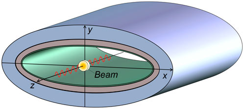
FIGURE 1. A relativistic charged particle beam with transversally Gaussian charge density moving at constant velocity on the axis of an infinitely long multilayer vacuum chamber with elliptical cross section.

In general, the electric and magnetic fields (E, H) in the presence of the particle beam in vacuum obey the Maxwell equations [1, 5]:

$\nabla \times \mathbf{E}=-{\mu }_0\frac{\partial \mathbf{H}}{\partial t},(1)$

$\nabla \times \mathbf{H}=\mathbf{J}+{\epsilon }_0\frac{\partial \mathbf{E}}{\partial t},(2)$

$\nabla \cdot \mathbf{E}=\frac{\rho }{{\epsilon }_0},(3)$

$\nabla \cdot \mathbf{H}=0.(4)$

where ɛ₀ and μ₀ denote the permittivity and the permeability of vacuum, respectively. In the frequency domain, the Maxwell Eqs. 1–4 can be transformed into

$\nabla \times \mathbf{E}=-j\omega {\mu }_0\mathbf{H},(5)$

$\nabla \times \mathbf{H}=\mathbf{J}+j\omega {\epsilon }_0\mathbf{E},(6)$

$\nabla \cdot \mathbf{E}=\frac{\rho }{{\epsilon }_0},(7)$

$\nabla \cdot \mathbf{H}=0.(8)$

Here we assume the time dependence e^jωt with an angular frequency ω = 2πf. When one consider only a particular harmonic component, the charge and current densities are written as

$\rho \left(x,y,z,t\right)={\rho }_{\perp }\left(x,y\right)e^{j\left(\omega t-kz\right)},(9)$

$\mathbf{J}\left(x,y,z,t\right)=J_z\left(x,y\right)e^{j\left(\omega t-kz\right)}{\mathbf{e}}_z,(10)$

respectively, where k = ω/v is the wave number, J_z = ρ_⊥βc, ρ_⊥ is the transverse charge density distribution function. The electric and magnetic fields are also written as:

$\mathbf{E}\left(x,y,z,t\right)=\mathbf{E}\left(x,y\right)e^{j\left(\omega t-kz\right)},(11)$

$\mathbf{H}\left(x,y,z,t\right)=\mathbf{H}\left(x,y\right)e^{j\left(\omega t-kz\right)},(12)$

respectively. From the frequency domain Maxwell Eqs. 5–8, we can obtain the following inhomogeneous wave equations of the electric field E = (E_x, E_y, E_z) and magnetic field H = (H_x, H_y, H_z) [1]:

${\nabla }^2\mathbf{E}+{\omega }^2{\epsilon }_0{\mu }_0\mathbf{E}=\frac{\nabla \rho }{{\epsilon }_0}+j\omega {\mu }_0\mathbf{J},(13)$

${\nabla }^2\mathbf{H}+{\omega }^2{\epsilon }_0{\mu }_0\mathbf{H}=-\nabla \times \mathbf{J}.(14)$

Substituting Eqs. 9–12 into Eqs. 13, 14 leads to

$\frac{{\partial }^2{E}_x}{\partial x^2}+\frac{{\partial }^2{E}_x}{\partial y^2}-\frac{k^2}{{\gamma }^2}{E}_x=\frac{1}{{\epsilon }_0}\left(\frac{\partial {\rho }_{\perp }}{\partial x}\right),(15)$

$\frac{{\partial }^2{E}_y}{\partial x^2}+\frac{{\partial }^2{E}_y}{\partial y^2}-\frac{k^2}{{\gamma }^2}{E}_y=\frac{1}{{\epsilon }_0}\left(\frac{\partial {\rho }_{\perp }}{\partial y}\right),(16)$

$\frac{{\partial }^2{E}_z}{\partial x^2}+\frac{{\partial }^2{E}_z}{\partial y^2}-\frac{k^2}{{\gamma }^2}{E}_z=-\frac{jk}{{\epsilon }_0{\gamma }^2}{\rho }_{\perp },(17)$

$\frac{{\partial }^2{H}_x}{\partial x^2}+\frac{{\partial }^2{H}_x}{\partial y^2}-\frac{k^2}{{\gamma }^2}{H}_x=-\frac{\partial J_z}{\partial y},(18)$

$\frac{{\partial }^2{H}_y}{\partial x^2}+\frac{{\partial }^2{H}_y}{\partial y^2}-\frac{k^2}{{\gamma }^2}{H}_y=\frac{\partial J_z}{\partial x},(19)$

$\frac{{\partial }^2{H}_z}{\partial x^2}+\frac{{\partial }^2{H}_z}{\partial y^2}-\frac{k^2}{{\gamma }^2}{H}_z=0,(20)$

where $\gamma ={(1-{\beta }^2)}^{-1/2}$ is the Lorentz factor. As described later, we are interested in Eq. 17 to calculate the coupling impedance.

2.2 Boundary conditions

To model the walls of a vacuum chamber, one needs to enforce the boundary condition. In the case of PEC walls, we use the PEC boundary condition (BC) as follows [1, 5]:

$\mathbf{n}\times \mathbf{E}=0.(21)$

For a smooth wall of finite conductivity, we replace the PEC-BC by the Leontovich boundary condition or SIBC [5, 26]:

$\mathbf{n}\times \mathbf{E}=Z_s\left(\omega \right)\mathbf{n}\times \mathbf{n}\times \mathbf{H},(22)$

where n is the outward unit vector normal to the wall surface and $Z_s\left(\omega \right)$ is called as the surface impedance, which is complex. When Z_s = 0, Eq. 22 can be reduced to the PEC-BC Eq. 21. Note that Eq. 22 is enforced only on the innermost wall of the chamber. In the field solution, all the domain outside the innermost wall is assumed to be filled by PEC. This can be also regarded as the assumption of infinitely thick PEC wall. Therefore, the field is zero outside the innermost chamber wall. This surface impedance concept can be widely used for the impedance modeling in particle accelerators. See e.g. [29].

For later reference, we summarize Z_s in some special cases. As a well-known example, the normal skin effect in a chamber wall with infinite thickness can be modeled with [5, 18, 26].

$Z_s\left(\omega \right)=\sqrt{\frac{j\omega {\mu }_0}{{\sigma }_c+j\omega {\epsilon }_0}}.(23)$

where σ_c is the static (dc) conductivity. For a multilayer structure, the transmission line theory [18] can be used to obtain its surface impedance in Eq. 22. The same approach as Ref. [18] is adapted in this work. As a result, for a three-layer structure with dc conductivities σ_i and thicknesses d_i (i = 1, 2, 3, respectively), Z_s on the inner wall is given by

$Z_s=Z_1\cdot \frac{Z_{i2}+Z_1\tanh \left({\gamma }_1{d}_1\right)}{Z_1+Z_{i2}\tanh \left({\gamma }_1{d}_1\right)},(24)$

$Z_{i2}=Z_2\cdot \frac{Z_{i3}+Z_2\tanh \left({\gamma }_2{d}_2\right)}{Z_2+Z_{i3}\tanh \left({\gamma }_2{d}_2\right)},(25)$

$Z_{i3}=Z_3\cdot \frac{Z_0+Z_3\tanh \left({\gamma }_3{d}_3\right)}{Z_3+Z_0\tanh \left({\gamma }_3{d}_3\right)},(26)$

where Z₀ is the free space impedance and Z_i and γ_i are the intrinsic impedance and the propagation constant of ith layer material, respectively, given by

$Z_i=\sqrt{\frac{j\omega {\mu }_0}{{\sigma }_i+j\omega {\epsilon }_0}},(27)$

${\gamma }_i=\sqrt{j\omega {\mu }_0\left({\sigma }_i+j\omega {\epsilon }_0\right)}.(28)$

Note that the vacuum regions are assumed to be inside the innermost wall surface and also outside the outermost wall surface.

Figure 2 shows surface impedances obtained with Eq. 23 for stainless steel (SS), copper (Cu), and nonevaporable getter (NEG) and a surface impedance calculated with Eq. 24 for a three-layer structure with the same conductivities. The materials used from external to inner layer are SS, Cu and NEG with the corresponding dc conductivities σ₃ = 0.14 × 10⁷ S/m, σ₂ = 5.88 × 10⁷ S/m, σ₁ = 0.55 × 10⁵ S/m. Layer thicknesses are d₃ = 1 mm for SS, d₂ = 1 μm for Cu and d₁ = 1 μm for NEG, respectively. As well known, for good conductors, Eq. 23 can be simplified as

$Z_s\left(\omega \right)=\left(1+j\right)\sqrt{\frac{Z_0\omega }{2{\sigma }_{c}c}}.(29)$

FIGURE 2

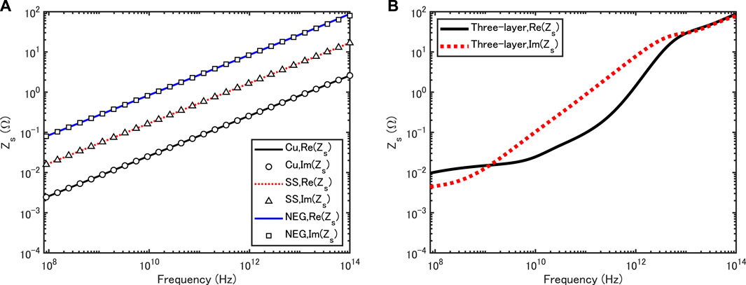
FIGURE 2. Surface impedances for the smooth wall of SS, Cu, NEG (A) and for the inner wall of the three-layer structure (B).

Therefore, the curve of the real part of the surface impedance agree with that of the imaginary one for Cu, SS and NEG, respectively. By contrast, for the three-layer structure, the frequency dependency of the real part is quite different from that of the imaginary one.

2.3 Kirchhoff’s boundary integral representation of electromagnetic field

The electromagnetic field in an infinitely long vacuum chamber can be also expressed in Kirchhoff’s boundary integral representation as [30].

$\mathbf{E}={\mathbf{E}}_b-{\nabla }_{\perp }\varphi -j\omega \mathbf{A}-\frac{1}{{\epsilon }_0}{\nabla }_{\perp }\times \mathbf{F},(30)$

$\mathbf{H}={\mathbf{H}}_b-{\nabla }_{\perp }{\varphi }_m-j\omega \mathbf{F}+\frac{1}{{\mu }_0}{\nabla }_{\perp }\times \mathbf{A}(31)$

with the vector and scalar potentials

$\mathbf{A}\left(\mathbf{r}\right)={\mu }_0{\int }_{C}G\left(\mathbf{r},{\mathbf{r}}^{\prime }\right)\mathbf{K}\left({\mathbf{r}}^{\prime }\right)d{\mathbf{r}}^{\prime },(32)$

$\mathbf{F}\left(\mathbf{r}\right)={\epsilon }_0{\int }_{C}G\left(\mathbf{r},{\mathbf{r}}^{\prime }\right)\mathbf{M}\left({\mathbf{r}}^{\prime }\right)d{\mathbf{r}}^{\prime },(33)$

$\varphi \left(\mathbf{r}\right)=\frac{1}{{\epsilon }_0}{\int }_{C}G\left(\mathbf{r},{\mathbf{r}}^{\prime }\right)\sigma \left({\mathbf{r}}^{\prime }\right)d{\mathbf{r}}^{\prime },(34)$

${\varphi }_m\left(\mathbf{r}\right)=\frac{1}{{\mu }_0}{\int }_{C}G\left(\mathbf{r},{\mathbf{r}}^{\prime }\right)\eta \left({\mathbf{r}}^{\prime }\right)d{\mathbf{r}}^{\prime },(35)$

and the boundary conditions

$\mathbf{n}\times \mathbf{E}=-\mathbf{M},(36)$

$\mathbf{n}\times \mathbf{H}=\mathbf{K},(37)$

$\mathbf{n}\cdot \mathbf{E}=\sigma /{\epsilon }_0,(38)$

$\mathbf{n}\cdot \mathbf{H}=\eta /{\mu }_0,(39)$

and Green’s function [1].

$G\left(\mathbf{r},{\mathbf{r}}^{\prime }\right)=\frac{1}{2\pi }{K}_0\left(k_{r}R\right),R=\left|\mathbf{r}-{\mathbf{r}}^{\prime }\right|,k_r=k/\gamma ,(40)$

where (E_b, H_b) are the beam self-fields, ${\nabla }_{\perp }^2=\frac{{\partial }^2}{\partial x^2}+\frac{{\partial }^2}{\partial y^2}$ is the two-dimensional (2D) Laplacian operator, r = (x, y) is the observation point in the bounded vacuum region, r′ is the point on the boundary surface, n is the inner unit vector normal to the inner wall surface C, K₀ is the modified Bessel function of the second kind of order zero, (K, σ) are the electric surface current and charge densities and (M, η) are the magnetic surface current and charge densities.

The above integral representation clearly shows that the total electromagnetic fields (E, H) can be expressed as a superposition of the beam self-fields and the boundary integrals over the surface charges and currents on the chamber walls. See Ref. [30] for more detailed discussions on Eqs. 30, 31.

Here we should mention the perturbative treatment of magnetic field; the magnetic field on resistive walls is assumed to be the same as that on PEC walls. In this case, M = 0 and η = 0. Therefore, to compute the magnetic field in the perturbative model, one uses

$\mathbf{H}={\mathbf{H}}_b+\frac{1}{{\mu }_0}{\nabla }_{\perp }\times \mathbf{A}(41)$

together with Eq. 37. In the previous study [28], the boundary data for PINN was generated with Eq. 22 and Eq. 41

Unlike Ref. [28], in this paper, boundary data for PINN are generated with the nonperturbative model based on Eqs. 30, 31 including Eq. 22 with Eq. 23 or 24.

3 Physics-informed neural network method

3.1 Data and equation scaling

For calculating the electromagnetic field in particle accelerators and the beam coupling impedance, we will deal with different magnitudes of input and output. For example, the field magnitude may vary largely within a vacuum chamber under consideration or in a frequency range of interest. The real part of the field can be also different from the imaginary one due to the frequency dependence of a surface impedance. In such cases, we have to deal with a dataset carefully. Using a raw dataset can lead to slow convergence of a gradient-based optimizer. To avoid this, we need to scale the input, output and PDE in an appropriate way. It should be mentioned that this basic idea was first described in Ref. [27]. Although the final scaled form of the PDE Eq. 17 was given in Ref. [28], its derivation was omitted. In the following, we present a detailed formulation for the data and equation scaling.

Let us consider modeling a vacuum chamber geometry in Cartesian coordinates. The x-axis and y-axis are scaled with typical chamber dimensions (s_x, s_y) such as radius, height and width as

$\bar{x}=\frac{x}{s_x},\bar{y}=\frac{y}{s_y}.(42)$

We then scale the sampling points (input) with Eq. 42 and transform the PDE Eq. 17 into

$\frac{1}{s_x^2}\frac{{\partial }^2{E}_z}{\partial {\bar{x}}^2}+\frac{1}{s_y^2}\frac{{\partial }^2{E}_z}{\partial {\bar{y}}^2}-\frac{k^2}{{\gamma }^2}{E}_z=-\frac{jk}{{\epsilon }_0{\gamma }^2}{\rho }_{\perp }.(43)$

Next, by scaling the field E_z (output) as

${\bar{E}}_z=\frac{E_z}{E_0},(44)$

we obtain

$\frac{1}{s_x^2}\frac{{\partial }^2{\bar{E}}_z}{\partial {\bar{x}}^2}+\frac{1}{s_y^2}\frac{{\partial }^2{\bar{E}}_z}{\partial {\bar{y}}^2}-\frac{k^2}{{\gamma }^2}{\bar{E}}_z=-\frac{jk}{{\epsilon }_0{\gamma }^2{E}_0}{\rho }_{\perp },(45)$

where ρ_⊥ is given by

${\rho }_{\perp }=\frac{Q}{2\pi {\sigma }_x{\sigma }_y}{e}^{-\frac{{\left(x-x_c\right)}^2}{2{\sigma }_x^2}-\frac{{\left(y-y_c\right)}^2}{2{\sigma }_y^2}},(46)$

where (σ_x, σ_y) is the Gaussian rms size in the x- and y-direction and (x_c, y_c) is the center position in the transverse plane. Finally, by setting s_x = s_y = s₀, introducing a new parameter B and choosing E₀ as

$E_0=q_n{s_0}^2\frac{k}{B{\epsilon }_0{\gamma }^2},q_n=\frac{Q}{2\pi {\sigma }_x{\sigma }_y},(47)$

we can derive a scaled PDE as follows:

$\frac{{\partial }^2{\bar{E}}_z}{\partial {\bar{x}}^2}+\frac{{\partial }^2{\bar{E}}_z}{\partial {\bar{y}}^2}-\frac{{\bar{k}}^2}{{\gamma }^2}{\bar{E}}_z=-jB\bar{\rho },(48)$

$\bar{\rho }=\exp \left[-\frac{{\left(\bar{x}{s}_0-x_c\right)}^2}{2{\sigma }_x^2}-\frac{{\left(\bar{y}{s}_0-y_c\right)}^2}{2{\sigma }_y^2}\right],(49)$

where $\bar{k}=k{s}_0$ and $\bar{\rho }={\rho }_{\perp }/q_n$ denotes the scaled charge density distribution. Throughout this paper, B = 1 is empirically chosen. Note that γ and $\bar{\rho }$ are included even in the scaled PDE Eq. 48, which has the same form as the original PDE Eq. 17.

As the scaled boundary condition for ${\bar{E}}_z$, we adapt

${\bar{E}}_z=E_l/E_0,(50)$

where E_l is the longitudinal electric field on the wall surface obtained with the recently proposed boundary element method (BEM) [30]. Note that, as already mentioned in Section 2.3, the nonperturbative model is used to obtain E_l in Eq. 50.

We highlight the effect of the above data and equation scaling by comparing Eq. 48 with Eq. 17. The right-hand side (RHS) of Eq. 17 will be relatively large due to the existence of ɛ₀ ≈ 8.854 × 10^–12 [F/m]. In addition, the RHS depends on the wavenumber k or the frequency f. These are unpreferable for using a gradient-based optimizer. By contrast, in the presented formulation Eqs. 42–50, the RHS of (48) is characterized by $B\bar{\rho }$ and it remains unchanged over a frequency range of interest. This feature is preferable for calculating the beam coupling impedance in the frequency domain and for maintaining the accuracy of trained NNs over a frequency range. In fact, this scaling has been successfully applied to all benchmark examples in this study. The presented scaling scheme is performed as pre-processing and post-processing.

Note that the physics of the electromagnetic field self-generated by the beam in a vacuum chamber can be described by Eqs 48, 50.

3.2 Deep learning

Let us consider solving the derived PDE via a new class of deep learning, termed as PINN [24, 25]. A deep neural netowrk (DNN) is used to approximate the solution of Eq. 48. This is often called as a solution surrogate. In addition, to train this DNN, we take the output of a DNN, define a network associated to the residual of Eqs 48, 50 and calculate the residual value (called a loss function). Note that differential operators in this residual network are calculated using the automatic differentiation. Therefore, unlike traditional numerical methods, our approach does not need to define (and generate) meshes inside the chamber. Physically, the space charge field has only a purely imaginary part, the resistive wall wake field has both real and imaginary parts. Therefore, the DNN also has two outputs $\left({\widehat{E}}_r,{\widehat{E}}_i\right)$ corresponding to the real (r) and imaginary 1) parts of ${\bar{E}}_z$. A schematic picture of constructed PINN including the DNN and the residual network is illustrated in Figure 3. The inputs of the DNN are sampling points $\left({\bar{x}}_p,{\bar{y}}_p\right)$ in the scaled xy plane. We assume that the beam traverses inside the chamber and the field is zero outside the chamber. The approach described here works well especially for smooth transverse charge density as in (49).

FIGURE 3

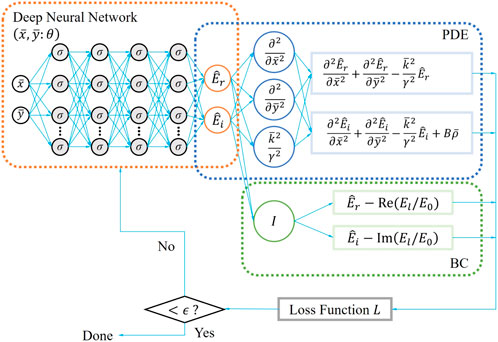
FIGURE 3. Physics-informed neural network.

Our algorithm is summarized in the following list.

1) Set up a computational domain, the boundary condition, physical constants, beam parameters, source domain, and the scaling parameters.

2) Generate randomly sampled points (or regular or irregular grid points) within the computational domain surrounded by the innermost wall. No sampling point is generated outside the domain.

3) Construct a DNN with two outputs ${\widehat{E}}_r\left(\bar{x},\bar{y};\theta \right),{\widehat{E}}_i\left(\bar{x},\bar{y};\theta \right)$ as a solution surrogate of the scaled PDE ${\bar{E}}_z\left(\bar{x},\bar{y}\right)={\bar{E}}_r\left(\bar{x},\bar{y}\right)+j{\bar{E}}_i\left(\bar{x},\bar{y}\right)$, where θ is a vector containing all weights w and bias b in the neural network to be trained, σ denotes an activation function.

4) Define the loss function L including Eqs 48, 50

5) Train the constructed DNN to find the best parameters θ by minimizing L via the L-BFGS algorithm [31] as a gradient-based optimizer, until L is smaller than a threshold ϵ.

6) Calculate the original field (unscaled) from ${\widehat{E}}_z\left(x,y;\theta \right)=E_0{\widehat{E}}_r\left(x/s_0,y/s_0;\theta \right)+j{E}_0{\widehat{E}}_i\left(x/s_0,y/s_0;\theta \right)$ using the trained DNN.

In this method, the loss function L is defined by

$L=w_r^d{L}_r^d+w_r^b{L}_r^b+w_i^d{L}_i^d+w_i^b{L}_i^b,(51)$

$L_r^d=\frac{1}{N_d}\sum _{p=1}^{N_d}{\left|f_r\left(x_p,y_p;\theta \right)\right|}^2,L_i^d=\frac{1}{N_d}\sum _{p=1}^{N_d}{\left|f_i\left(x_p,y_p;\theta \right)\right|}^2,(52)$

$L_r^b=\frac{1}{N_b}\sum _{p=1}^{N_b}{\left|g_r\left(x_p,y_p;\theta \right)\right|}^2,L_i^b=\frac{1}{N_b}\sum _{p=1}^{N_b}{\left|g_i\left(x_p,y_p;\theta \right)\right|}^2,(53)$

$f_r=\frac{{\partial }^2{\widehat{E}}_r}{\partial {\bar{x}}^2}+\frac{{\partial }^2{\widehat{E}}_r}{\partial {\bar{y}}^2}-\frac{{\bar{k}}^2}{{\gamma }^2}{\widehat{E}}_r,f_i=\frac{{\partial }^2{\widehat{E}}_i}{\partial {\bar{x}}^2}+\frac{{\partial }^2{\widehat{E}}_i}{\partial {\bar{y}}^2}-\frac{{\bar{k}}^2}{{\gamma }^2}{\widehat{E}}_i+B\bar{\rho },(54)$

$g_r={\widehat{E}}_r-\text{Re}\left(E_l/E_0\right),g_i={\widehat{E}}_i-\text{Im}\left(E_l/E_0\right),(55)$

where p denotes the sampling point, N_d and N_b are the numbers of sampling points in the computational domain and on the boundary surface, respectively. $w_r^d$, $w_i^d$, $w_r^b$ and $w_i^b$ are the weights of the loss function. $L_{r/i}^d$ is the loss function related to the scaled PDE, and its minimization $\left(L_{r/i}^d\to 0\right)$ enforces Eq. 48 at a set of finite sampling points in the computational domain. $L_{r/i}^b$ is the loss function related to the SIBC, and its minimization $\left(L_{r/i}^b\to 0\right)$ enforces Eq. 50 at a set of finite sampling points on the boundary surface.

Throughout this study, a fully connected feedforward neural network was adapted, and four hidden layers and 30 neurons per layer were used. In deep learning, tanh, sigmoid, Rectified Linear Unit (ReLU) and Swish functions are commonly used as nonlinear activation functions. See e.g., Refs. [32, 33]. Smooth activation functions are required in PINN. Since ReLU is not differentiable at the origin, we do not choose it here. For this study, the Swish function [32] is used, because it tends to work well for various chamber geometries, compared to the tanh and sigmoid functions. This activation function was not used in the previous studies [27, 28]. B = 1 and ($w_r^d$, $w_i^d$, $w_r^b$, $w_i^b$)=(10,1,10,1) were chosen.

3.3 Impedance computation

After training the neural network, one can predict the field ${\widehat{E}}_z\left(x,y;\theta \right)$ for any position (x, y) in a vacuum chamber. In order to estimate integrated effect of the field on the beam in the frequency domain, the concept of coupling impedance is commonly used in accelerator physics. Here the coupling impedance is defined as [4].

$Z_{\Vert }\left(x,y\right)=-\frac{{\widehat{E}}_z\left(x,y;\theta \right)}{I},(56)$

where I = Qβc is the total beam current. The coupling impedance (per unit length) at any position inside the source domain of (46) is obtained from (56). Although one can define the impedance averaged over the source domain, its evalution is out of the present paper. This paper focuses on the local impedance defined in (56).

4 Results and discussion

To show the feasibility of the presented approach, we apply it to the impedance analysis of multilayer vacuum chambers with circular and elliptical cross section. Here, we assume the vertical dimension (height) h = 2b = 10 mm as in [20] and γ = 10,000, which is corresponding to the ultrarelativistic case. The PINN-predicted results are verified in comparison with simulation results of the recently developed BEM.

First, the coupling impedance of a circular vacuum chamber of infinite thickness is simulated for different wall materials (N_d, N_b)=(1,578, 200) was used for a circular chamber. The domain and boundary sampling points were generated as in Figure 4, where the coordinates are scaled with s₀ = 5 mm.

FIGURE 4

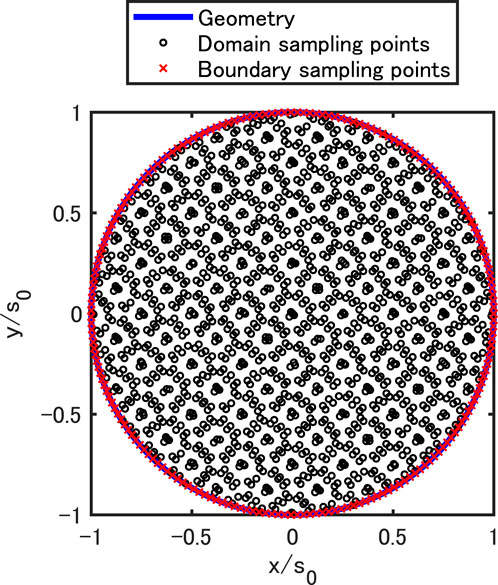
FIGURE 4. Generation of sampling points in a domain surrounded by the innermost wall of a circular vacuum chamber.

Figure 5 shows the coupling impedances of a round Gaussian beam with σ_x = σ_y = σ_r = 0.5 mm on the axis of the circular chamber for copper (Cu), stainless steel (SS) and nonevaporable getter (NEG). As expected, both the real and imaginary parts of the coupling impedance decrease at each frequency point as σ_c increases. For example, the impedance of the copper vacuum chamber is smaller than those of the other two. For each σ_c, at low frequencies, the frequency dependence of the real part is very similar to that of the imaginary part. This feature originates from the frequency dependence of Eq. 23 and also the fact that the magnetic field on the resistive wall is very similar to that on the PEC wall in a limited frequency range. However, at high frequencies, the real part is different from the imaginary one. This is not surprising. From the impedance theory [5], it is known that the above low frequency characteristic is valid for $\left(|Z_s|\omega b\right)/\left(2c{Z}_0\right)\ll 1$. In this example, it reads f ≪7.2 THz for Cu and b = 5mm, f ≪1.8 THz for SS and b = 6mm, f ≪0.71 THz for NEG and b = 5mm, respectively. This feature is confirmed in Figure 5. Note that the geometry parameter b and the dc conductivity σ_c are also included in this condition. We also find good agreement between PINN and BEM results in both the real and imaginary parts. This means that the wideband behavior of coupling impedance due to both the geometric effect and the skin effect characterized by Eq. 23 is reproduced in the PINN simulations.

FIGURE 5

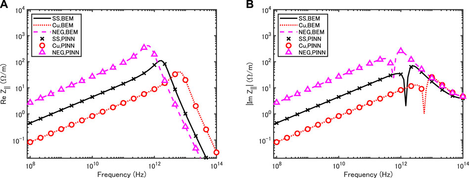
FIGURE 5. Coupling impedances of a round Gaussian beam with σ_r = 0.5 mm moving on the axis of a circular vacuum chamber with infinite thickness for three different wall materials: copper (Cu), stainless steel (SS), nonevaporable getter (NEG). The copper and NEG chambers have radius of 5 mm and the SS chamber has radius of 6 mm. Real part (A) and imaginary part (B).

Figure 6 demonstrates a direct comparison of perturbative and nonperturbative models in the coupling impedance for the circular vacuum chamber with the NEG wall as shown in Figure 5. As expected, the perturbative impedance agrees with the nonperturbative one for f ≪0.71 THz while the perturbative impedance is different from the nonperturbative one at higher frequencies. This result means that the magnetic field on the resistive wall is not same as that on the PEC walls at higher frequencies. In other words, the effect of finite conductivity on the magnetic field cannot be negligible as the frequency increases. This demonstrates that the nonperturbative effect is reproduced in the PINN framework.

FIGURE 6

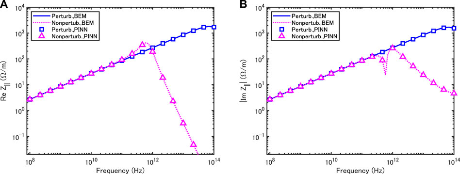
FIGURE 6. Comparison of the perturbative and nonperturbative models in the coupling impedances of a round Gaussian beam with σ_r = 0.5 mm moving on the axis of a circular vacuum chamber with infinite thickness for NEG. The NEG chamber has radius of 5 mm. Real part (A) and imaginary part (B).

Next, the coupling impedance of a three-layer circular vacuum chamber is simulated for different inner coating thicknesses. The same domain and boundary sampling points as in Figure 4 and (N_d, N_b)=(1,578, 200) were used here.

Figure 7 shows the coupling impedances of a round Gaussian beam with σ_r = 0.5 mm on the axis of a circular chamber of inner radius 5 mm and outer radius 6 mm with the three-layer structure of SS, Cu and NEG. For each of different NEG thicknesses of 0.01, 0.1, 1 and 10μm, the frequency dependence of the real part of the coupling impedance is quite different from that of the imaginary part. For all NEG layer thicknesses, we find good agreement between PINN and BEM results in both the real and imaginary parts. Note that a characteristic high frequency peak in the real part is observed for the inner layer thickness of 1 μm. This peak was originally found in the impedance theory of the circular multilayer tube [20]. Our result shows the applicability of PINN to the impedance modeling of a circular vacuum chamber with three-layer structure.

FIGURE 7

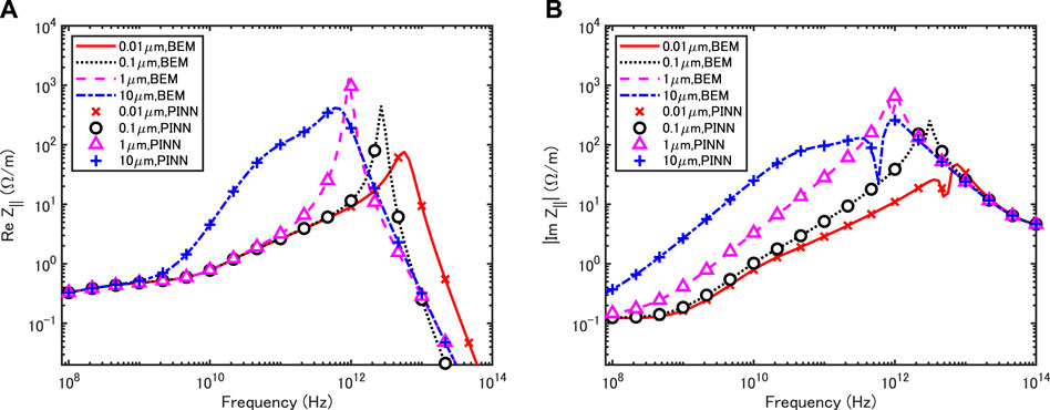
FIGURE 7. Coupling impedances of a round Gaussian beam with σ_r = 0.5 mm moving on the axis of the circular vacuum chamber with the three-layer structure of copper (Cu), stainless steel (SS), nonevaporable getter (NEG). Real part (A) and imaginary part (B).

Finally, the coupling impedance of an elliptical multilayer vacuum chamber is simulated. The chamber is assumed to have the major axis a = 9 mm and the minor axis b = 5 mm at the inner surface. This application is not shown in our previous study [28]. For this elliptical chamber, the domain and boundary sampling points shown in Figure 8 are generated with (N_d, N_b)=(2,845, 360).

FIGURE 8

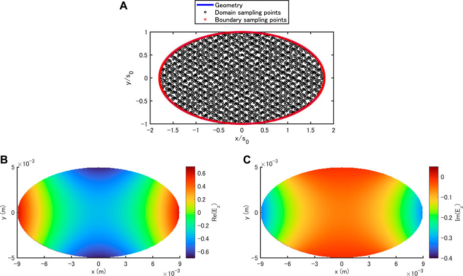
FIGURE 8. PINN-simulated field distribution E_z over a domain surrounded by the innermost wall of a three-layer elliptical vacuum chamber (A) sampling points (B) real part (C) imaginary part.

Figure 9 demonstrates a direct comparison of nonperturbative and perturbative models in the coupling impedance of a Gaussian round beam with σ_r = 0.5 mm for the elliptical vacuum chamber with the same three-layer structure as shown in Figure 2. As expected, the perturbative results (right) are quite different from the nonperturbative ones (right); no resonant peak is observed in the perturbative result. This comparison clearly show even for the three-layer elliptical vacuum chamber the nonperturbative effect is reproduced in the PINN framework.

FIGURE 9

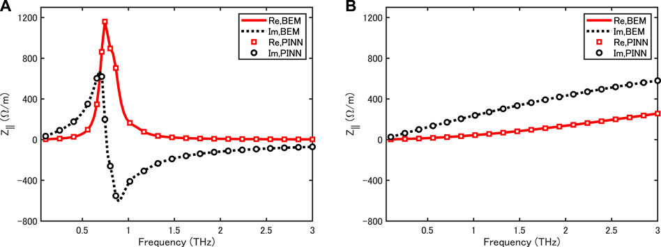
FIGURE 9. Coupling impedance of a round Gaussian beam with σ_r = 0.5 mm for an elliptical vacuum chamber with the three-layer structure of copper (Cu), stainless steel (SS), nonevaporable getter (NEG) (A) nonperturbative model (B) perturbative model.

In the left side of Figure 9, the frequency dependence of the real part of the coupling impedance is different from that of the imaginary part. The highest peak in the real part is at f ≈ 0.74 THz. In the bottom of Figure 8, we display the PINN-predicted field distribution E_z over a domain surrounded by the innermost wall at its peak frequency. Unlike the case of a circular chamber in Ref. [28], the field distribution shown here is non-uniform over the elliptical cross section. This feature is also confirmed from the field curves along x- and y-axes in Figure 10. The effect of elliptical cross section on the field is demonstrated in these results.

FIGURE 10

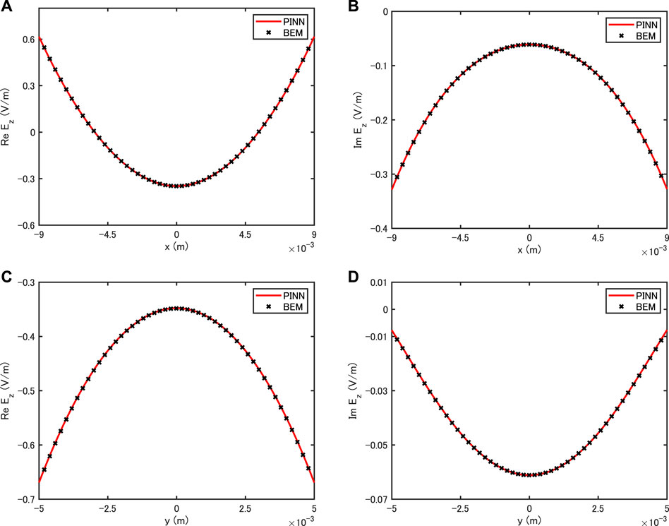
FIGURE 10. Comparison of electric field in a three-layer elliptical vacuum chamber calculated with PINN and BEM (A) Re (E_z) along x-axis at y = 0 (B) Im (E_z) along x-axis at y = 0, and (C) Re (E_z) along y-axis at x = 0 and (D) Im (E_z) along y-axis at x = 0.

We find good agreement between PINN and BEM results for both the real and imaginary parts of the impedance in Figure 9 and also for the electric field distributions along the x- and y-axes in Figure 10. These results clearly show the applicability of PINN to multilayer vacuum chambers other than the circular one.

5 Conclusion

This paper has presented a deep learning-based approach for calculating the wakefields of a relativistic charged particle beam with transversally Gaussian charge density distribution in an infinitely long multilayer vacuum chamber with arbitrary cross section. This approach is based on PINN and SIBC of a multilayer structure derived from TL theory. It has been successfully applied to circular and elliptical vacuum chambers with the three-layer structure of SS, Cu and NEG in the nonperturbative model. The PINN results have been cross-checked with the recently developed BEM ones. The effects of chamber geometries and three-layer structure on the coupling impedance have been demonstrated in the framework of PINN.

In this study, a transversally Gaussian charge density distribution is assumed. Therefore, the presented method cannot model a uniform charge density with hard edges, point and ring charges as often used in accelerator physics. A solution to this limitation will be presented in near future. On the other hand, the method has been formulated for two-dimensional problems in the frequency domain. As future works, its extensions to three-dimensional problems and the time domain are under consideration.

Data availability statement

The original contributions presented in the study are included in the article/Supplementary Material, further inquiries can be directed to the corresponding author.

Author contributions

KF confirms being the solo contributor of this work and has approved it for publication.

Conflict of interest

The author declares that the research was conducted in the absence of any commercial or financial relationships that could be construed as a potential conflict of interest.

Publisher’s note

All claims expressed in this article are solely those of the authors and do not necessarily represent those of their affiliated organizations, or those of the publisher, the editors and the reviewers. Any product that may be evaluated in this article, or claim that may be made by its manufacturer, is not guaranteed or endorsed by the publisher.

References

1. Jackson JD. Classical electrodynamics. New York: Wiley (1998).

Google Scholar

2. Chao AW. Physics of collective beam instabilities in high energy accelerators. New York: Wiley (1993).

Google Scholar

3. Ng KY. Physics of intensity dependent beam instabilities. Singapore: World Scientific (2006).

Google Scholar

4. Zotter BW, Kheifets SA. Impedance and wakes in high-energy accelerators. Singapore: World Scientific (1998).

Google Scholar

5. Stupakov G, Penn G. Classical mechanics and electromagnetism in accelerator physics. Cham: Springer International Publishing AG (2018).

Google Scholar

6. Morton PL, Neil VK, Sessler AM. Wake fields of a pulse of charge moving in a highly conducting pipe of circular cross section. J Appl Phys (1966) 37:3875–83. doi:10.1063/1.1707941

CrossRef Full Text | Google Scholar

7. Zotter B. Longitudinal instabilities of charged particle beams inside cylindrical walls of finite thickness. Part Accel (1970) 1:311–26.

Google Scholar

8. Henke H, Napoly O. Wake fields between two parallel resistive plates. In: Proc. 2nd European Particle Accelerator Conference; Nice, France (1990). p. 1046–8.

Google Scholar

9. Gluckstern R, van Zeijts J, Zotter B. Coupling impedance of beam pipes of general cross section. Phys Rev E (1993) 47:656–63. doi:10.1103/physreve.47.656

PubMed Abstract | CrossRef Full Text | Google Scholar

10. Gluckstern RL. Analytic methods for calculating coupling impedances. CERN Report No. 2000-011 (2000).

Google Scholar

11. Al-khateeb AM, Boine-Frankenheim O, Hasse RW, Hofmann I. Analytical calculation of the longitudinal space charge and resistive wall impedances in a smooth cylindrical pipe. Phys Rev E (2001) 63:026503. doi:10.1103/physreve.63.026503

PubMed Abstract | CrossRef Full Text | Google Scholar

12. Zimmermann F, Oide K. Resistive-wall wake and impedance for nonultrarelativistic beams. Phys Rev ST Accel Beams (2004) 7:044201. doi:10.1103/physrevstab.7.044201

CrossRef Full Text | Google Scholar

13. Bane KLF, Stupakov G. Resistive wall wakefield in the LCLS undulator beam pipe. In: Proc. 2005 Particle Accelerator Conference. Knoxville, Tennessee: IEEE (2005). p. 3390–2. See also SLAC-PUB-10707.

Google Scholar

14. Stupakov G. Resistive-wall wake for nonrelativistic beams revisited. Phys Rev Accel Beams (2020) 23:094401. doi:10.1103/physrevaccelbeams.23.094401

CrossRef Full Text | Google Scholar

15. Doliwa B, Arevalo E, Weiland T. Numerical calculation of transverse coupling impedances: Comparison to spallation neutron source extraction kicker measurements. Phys Rev ST Accel Beams (2007) 10:102001. doi:10.1103/physrevstab.10.102001

CrossRef Full Text | Google Scholar

16. Niedermayer U, Boine-Frankenheim O, Gersem HD. Space charge and resistive wall impedance computation in the frequency domain using the finite element method. Phys Rev ST Accel Beams (2015) 18:032001. doi:10.1103/physrevstab.18.032001

CrossRef Full Text | Google Scholar

17. Burov A, Lebedev V. Transverse resistive wall impedance for multi-layer round chamber. In: Proc. 2002 European Particle Accel. Conf.; Paris, France (2002). p. 1452–4.

Google Scholar

18. Vos L. The impedance of multi-layer vacuum chambers. CERN-AB 2003-093 (2003).

Google Scholar

19. Zotter B. New results on the impedance of resistive metal walls of finite thickness. CERN-AB 2005-043 (2005).

Google Scholar

20. Ivanyan M, Laziev E, Tsakanov V, Vardanyan A, Heifets S, Tsakanian A. Multilayer tube impedance and external radiation. Phys Rev ST Accel Beams (2008) 11:084001. doi:10.1103/physrevstab.11.084001

CrossRef Full Text | Google Scholar

21. Mounet N, Métral E. Impedance of two dimensional multilayer cylindrical and flat chambers in the non-ultrarelativistic case. In: Proc. HB2010; Morschach, Switzerland (2010). p. 353–7.

Google Scholar

22. Macridin A, Spentzouris P, Amundson J, Spentzouris L, McCarron D. Coupling impedance and wake functions for laminated structures with an application to the fermilab booster. Phys Rev ST Accel Beams (2011) 14:061003. doi:10.1103/physrevstab.14.061003

CrossRef Full Text | Google Scholar

23. Migliorati M, Palumbo L, Zannini C, Biancacci N, Vaccaro VG. Resistive wall impedance in elliptical multilayer vacuum chambers. Phys Rev Accel Beams (2019) 22:121001. doi:10.1103/physrevaccelbeams.22.121001

CrossRef Full Text | Google Scholar

24. Raissi M, Perdikaris P, Karniadakis GE. Physics-informed neural networks: A deep learning framework for solving forward and inverse problems involving nonlinear partial differential equations. J Comput Phys (2019) 378:686–707. doi:10.1016/j.jcp.2018.10.045

CrossRef Full Text | Google Scholar

25. Karniadakis GE, Kevrekidis IG, Lu L, Perdikaris P, Wang S, Yang L. Physics-informed machine learning. Nat Rev Phys (2021) 3:422–40. doi:10.1038/s42254-021-00314-5

CrossRef Full Text | Google Scholar

26. Senior TBA, Volakis JL. Approximate boundary conditions in electromagnetics. London: IEE Press (1995).

Google Scholar

27. Fujita K. Physics-informed neural network method for space charge effect in particle accelerators. IEEE Access (2021) 9:164017–25. doi:10.1109/access.2021.3132942

CrossRef Full Text | Google Scholar

28. Fujita K. Physics-informed neural network method for modelling beam-wall interactions. Electron Lett (2022) 58:390–2. doi:10.1049/ell2.12469

CrossRef Full Text | Google Scholar

29. Fujita K. Modeling of beam-wall interaction in a finite-length metallic pipe with multiple surface perturbations. IEEE J Multiscale Multiphys Comput Tech (2017) 2:237–42. doi:10.1109/jmmct.2017.2786864

CrossRef Full Text | Google Scholar

30. Fujita K. Impedance computation of cryogenic vacuum chambers using boundary element method. Phys Rev Accel Beams (2022) 25:064601. doi:10.1103/physrevaccelbeams.25.064601

CrossRef Full Text | Google Scholar

31. Liu DC, Nocedal J. On the limited memory BFGS method for large scale optimization. Math Program (1989) 45:503–28. doi:10.1007/bf01589116

CrossRef Full Text | Google Scholar

32. Ramachandran P, Zoph B, Le Q. Searching for activation functions. In: Proc. ICLR (2018).

Google Scholar

33. Aggarwal CC. Neural networks and deep learning. Cham: Springer International Publishing AG (2018).

Google Scholar