Data-driven modeling of beam loss in the LHC

In the Large Hadron Collider, the beam losses are continuously measured for machine protection. By design, most of the particle losses occur in the collimation system, where the particles with high oscilla-tion amplitudes or large momentum error are scraped from the beams. The particle loss level is typically optimized manually by changing control parameters, among which are currents in the focusing and defocusing magnets. It is generally challenging to model and predict losses based only on the control parameters, due to the presence of various (non-linear) effects in the system, such as electron clouds, resonance effects, etc., and multiple sources of uncertainty. At the same time understanding the influence of control parameters on the losses is extremely important in order to improve the operation and performance, and future design of accelerators. Prior work [1] showed that modeling the losses as an instantaneous function of the control parameters does not generalize well to data from a different year, which is an indication that the leveraged statistical associations are not capturing the actual mechanisms which should be invariant from 1 year to the next. Given that this is most likely due to lagged effects, we propose to model the losses as a function of not only instantaneous but also previously observed control parameters as well as previous loss values. Using a standard reparameterization, we reformulate the model as a Kalman Filter (KF) which allows for a flexible and efficient estimation procedure. We consider two main variants: one with a scalar loss output, and a second one with a 4D output with loss, horizontal and vertical emittances, and aggregated heatload as components. The two models once learned can be run for a number of steps in the future, and the second model can forecast the evolution of quantities that are relevant to predicting the loss itself. Our results show that the proposed models trained on the beam loss data from 2017 are able to predict the losses on a time horizon of several minutes for the data of 2018 as well and successfully identify both local and global trends in the losses.

1 Introduction

Excessively high beam losses in the Large Hadron Collider (LHC) [2, 3] can cause a quench in the superconducting magnets which will trigger a beam dump and a long recovery period to restore the nominal temperature. As a result, valuable time and hence integrated luminosity is lost for the physics experiments while the LHC needs to be refilled with a new beam. On the other hand, better control of losses guarantees more efficient operations, higher luminosity, and thus greater discovery potential. During the LHC run, the machine operators may change several parameters of the system, such as currents in the quadrupole, sextupole, and octupole magnets, in order to maximize the beam intensity and thus minimize the particle loss. Machine learning and statistical methods have been extensively used to analyze the data from accelerators and to improve operations [4–9]. It is possible to construct predictive models of the losses from the control parameters using standard ML techniques [1] based on LHC beam loss data within the same year, but the generalization of such approaches to the data of the next year was found to be challenging. A better understanding of the instantaneous and longer-term effects of control parameters on beam losses can help decrease the losses and improve the operations and performance output of the LHC. Furthermore, it can possibly lead to mitigation techniques for the particle losses for other existing machines as well as provide valuable input already during the design phase of potential future colliders, such as the Future Circular Collider (FCC) [10, 11]. At present, there is no accurate physics model for particle beam losses as a function of machine settings and control parameters. A statistical or machine learning model that would cover the possible scenarios of control parameters evolution could eventually be employed to find the optimal control policy. Using an optimized plan for the control parameters could significantly improve the performance of the accelerators. In what follows we make a step in this direction: the goal of this work is to improve the understanding of the effect of input parameters on losses and to propose an interpretable model which would be general and robust enough to generalize to beam loss data acquired in different years.

We assume that the two LHC beams evolve similarly under the change of control parameters disregarding possible beam coupling effects, and we concentrate on modeling the beam 1 losses. The majority of the losses occur in the collimation systems located in the beam cleaning areas at the Insertion Region (IR) 3 and IR7 of the accelerator, where the losses are recorded by beam loss monitors (BLM) [12]. The collimators at IR7 remove particles with large transverse oscillation amplitudes, whereas those at IR3 are responsible for removing the particles with a momentum error beyond a chosen threshold. Among the two collimator systems, the most active cleaning happens in IR7, therefore we concentrate on modeling of losses of beam 1 recorded by the BLM at IR7 and further refer to it as “the loss.”

Several additional important characteristics can be measured during the machine run, which cannot be directly controlled, but that contain information about hidden non-linear processes affecting the beam. Among such quantities are heatloads, that are a proxy to electron cloud effects [13], as well as horizontal and vertical emittances. The emittances describe the spread of the particles in phase space and are related to the mean physical dimension of the beam in the machine [14]. The emittance measurements are carried out in time along the beam and specific post-processing is used to estimate the average emittance of the whole beam. During the operation of the LHC, electron cloud can appear due to the acceleration of electrons in the beam pipe by the proton bunches, causing an avalanche process which leads to the heating of the beam pipe and magnets, to increased emittance and potentially to beam instabilities [15].

Tune variables are related to the frequency of betatronic oscillations in the machine. Tunes are corrected through a dedicated feedback system and mainly depend on the strength of the quadrupole magnets, although they can be also affected by the quadrupole component in the main dipoles, by the sextupole component from the main dipoles and sextupole corrector magnets [16].

As most of the non-linear effects in the beam physics are indirectly related to the change of input parameters it appears natural to rely on the information contained in the past observations. We therefore consider Vector AutoRegressive Moving Average models with eXogenous input variables (VARMAX) and compare them with models that relate the input variables directly to the losses. We train a common model on the data from multiple time series from one given year corresponding each to a different LHC fills with diverse filling schemes¹.

Available data: To construct and evaluate the predictive model of losses the observations of the losses along with other quantities measured during the LHC fills of the years 2017 and 2018 are available [17]. Observations are recorded with a frequency of 1 Hz. The fills start with the injection of the beam according to a selected filling scheme. We have selected the filling schemes which are occurring most frequently among all the encountered schemes in the data as we expected that the properties of the injected beam could vary depending on the type of injection. Altogether, for the selected schemes, the data of 105 fills are available in 2017, and 144 fills are recorded for 2018. We focus on the data for beam 1 during the “PRERAMP” beam mode of the machine fill. The “PRERAMP” beam mode occurs after the full beam has been injected and before starting the energy ramp process. During “PRERAMP,” measures are taken to prepare for the energy ramp, such as retracting the injection collimators, adjusting the feedback reference and loading other machine settings. During the “PRERAMP” mode machine is in stable conditions, and thus it should be supposedly the easiest beam mode to model losses. Nevertheless, on practice, it occurred to be challenging [1]. For each fill during the years 2017 and 2018 the time series of “PRERAMP” mode vary in length (see Figure 1).

FIGURE 1

FIGURE 1. Histogram of PRERAMP time series lengths for the years 2017 and 2018.

Throughout the paper, we assume that a logarithmic transformation is applied to the losses normalized by intensity. Further, we omit “log” and “normalized by intensity” while mentioning losses. The logarithmic transform is generally applied to reduce the skewness of the distribution (see the loss in original scale in Figure 2A and the log-transformed loss in Figure 2B). For the losses, the log-transformation is partially motivated by the fact that losses normalized by intensity are produced from the particle count data. For the convenience of further analysis, we assume that the log losses are Gaussian. Alternatively, one could follow the Generalized Linear Model approach, assuming the Poisson distribution of the count data, e.g. as in [18].

FIGURE 2

FIGURE 2. (A) original losses (normalized by intensity), (B) log-losses (normalized by intensity), for the years 2017 and 2018. The log-transform helps to reduce the skewness. Note that several modes on the pictures are due to changes of the losses level because of changes in control parameters, see e.g. Figure 3.

Several quantities are recorded during the experiment, among which we will use the following variables as the input/controlled parameters for the loss models.

• ${\mathcal{Q}}_x$ and ${\mathcal{Q}}_y$ — vertical and horizontal tunes,

• $\mathcal{C}$ — current in octupole magnets.

Non-controlled observed variables are

• $\mathcal{L}$ — logarithm of loss divided by intensity at BLM 6L7 for the beam 1,

• ${\mathcal{E}}_x$, ${\mathcal{E}}_y$ — horizontal and vertical emittance,

• e_c—sum of the heatload measurements over the 8 sectors of the LHC,

• τ—time since the beam injection.

Remark: Note that the tunes are actually controlled by quadrupole magnet currents, the field decays due to persistent currents and a feedback system that keeps the tune values measured with a Base-Band Tune (BBQ) measurement system at a constant value [19]. Although the control that we have over the tunes is an indirect one, we nonetheless treat the tunes (measured online in our dataset) as one of the control variables of the system. For the octupoles, we use the currents because there is no measurement of the tune spread associated with these elements. Also, time since the beam injection, though not controlled, is used as an input parameter.

For an example of evolution of the loss and other variables during the “PRERAMP” mode within one fill in the year 2017, see Figure 3. Typically, one significant modification of current and tunes occurs during “PRERAMP.”

FIGURE 3

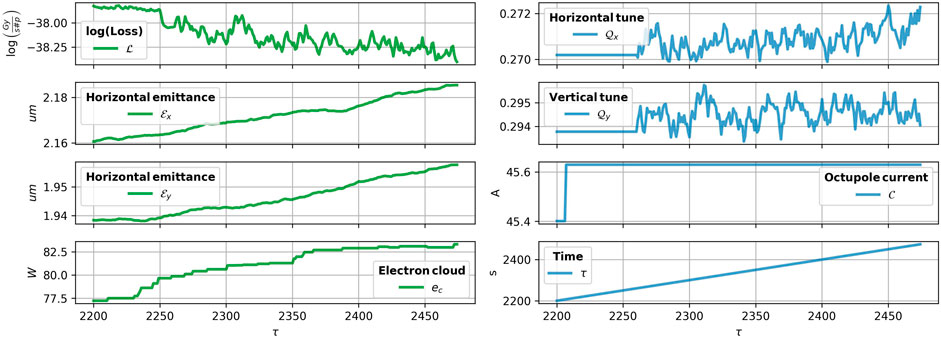
FIGURE 3. An example of PRERAMP mode time series for the fill 6,243 in 2017. The time series of vertical and horizontal tunes and octupole currents are shown in blue, observations of the loss, vertical and horizontal emittance and the sum of heatload measurements are shown in green.

The data for the years 2017 and 2018 differ in the ranges of input parameters used and in the level of losses: in Figure 4, non-controlled variables have different distributions, e.g. losses (Figure 4A) in 2017 were overall higher than in 2018; input variables, shown in Figure 5, had different ranges, e.g. see octupole current in Figure 5A, as well as increments of input variables in Figure 6, e.g. octupole current was only decreasing in 2018, both increasing and decreasing in 2017. Some of the control parameters, such as octupole current, change quite rarely, e.g. in the data of 2017, it changes from one level to another in “PRERAMP” time series only in half of the fills. This already suggests that applying the model trained on the data from 2017 to the data of 2018 require to extrapolate which is known to be quite challenging. We therefore privilege the use of simple (and thus robust) modeling techniques.

FIGURE 4

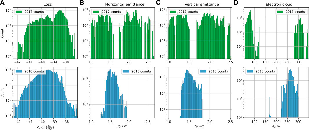
FIGURE 4. Histograms of the observations in 2017 and 2018. (A) Logarithm of loss normalized by intensity, (B) horizontal emittance, (C) vertical emittance, (D) heatload induced by electron cloud. Almost all the variables demonstrate different ranges of values for both years, e.g. see the sum of the heatloads.

FIGURE 5

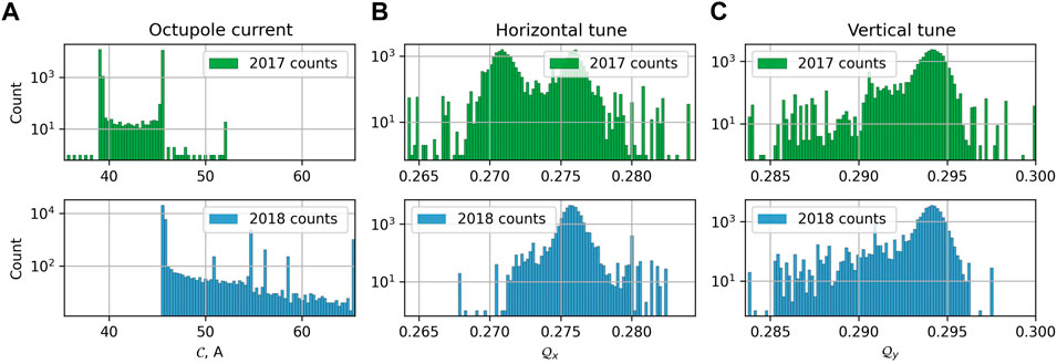
FIGURE 5. Histograms of the observations in 2017 and 2018. (A) Octupole current, (B) horizontal tune, (C) vertical tune. Almost all the variables demonstrate different ranges of values for both years, e.g. see the octupole current $\mathcal{C}$.

FIGURE 6

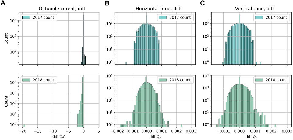
FIGURE 6. Histogram of increments of (A) octupole current, (B)horizontal tune and (C) vertical tune in 2017 and 2018. The fill 7,236 is a big outlier to the left in the histogram of octupole current in 2018.

Starting from the injection of the beam, multiple effects occur in the system, which cannot be fully described analytically, and have been so far observed in separate experiments, e.g. changes in the distribution of particle tunes in time due either to drift or to changes of the control parameters and for example associated with crossing resonance lines. Given the limited information about such events and about long-term dependence between control variables and losses, we consider a simple, but robust linear approach to model the dependence of losses on its prior history and on controlled and possibly uncontrolled variables. An example of such model in the 1D case which models losses as a function of tunes and octupole current would be of the form

$\begin{array}{cc}\hfill {\mathcal{L}}_t& ={\alpha }_1{\mathcal{L}}_{t-1}+{\alpha }_2{\mathcal{L}}_{t-2}+\dots \hfill \\ \hfill & +{\beta }_1{\mathcal{Q}}_{x,t-1}+{\beta }_2{\mathcal{Q}}_{x,t-2}+\dots \hfill \\ \hfill & +{\gamma }_1{\mathcal{Q}}_{y,t-1}+{\gamma }_2{\mathcal{Q}}_{y,t-2}+\dots \hfill \\ \hfill & +{\zeta }_1{\mathcal{C}}_{t-1}+{\zeta }_2{\mathcal{C}}_{t-2}+\dots \hfill \\ \hfill & +\text{\hspace{0.17em}noise}.\hfill \end{array}(1)$

with a general form of correlated noise process this is an instance of an autoregressive model with moving average and exogeneous variables, a so-called ARMAX model [20].

In a model of the form above, given that losses are closely related to emittances and will be affected by electron cloud, and in spite of the fact that these variables cannot be controlled, we chose to include them among the exogenous variables.

Finally, we will consider a multivariate time series model for the losses together with the emittances and electron cloud induced heatloads to try and predict their evolution jointly from controlled variables. This is motivated by the fact that we wish to obtain a model that captures the effect of the control variables so that if we rely on the values of emittances and electron cloud at some time t−l it should itself be predicted from the control variables at prior time points. This kind of multivariate extension is known as a vector ARMAX–or VARMAX–model.

To estimate the parameters of this type of model, we will exploit the relationship between VARMAX models and the Kalman Filter (KF).

The paper is organized as follows. In Section 2, after introducing more precisely the form of the different models we discuss VARMAX models and their relation to so-called state space models and in particular to the Kalman filter. Different parameterizations will lead us to consider a general KF with time-varying parameters, including a KF model with parameters depending on the input variables. We will consider different ways of regularizing the coefficients, and discuss a general Expectation-Maximization (EM) procedure for the estimation of parameters. Section 3 is devoted to the results of numerical experiments and to comparisons of the models.

2 Models

In this paper we consider several variants of the model described in Eq. 1.

KF1: First, we verify whether it is possible to construct a predictive model of the current losses as a function of the recent histories of the losses and of the control variables, as in KF1. More precisely, we consider a 1D linear model of losses.

$\begin{array}{ll}\hfill {\mathcal{L}}_t& ={\alpha }_1{\mathcal{L}}_{t-1}+{\alpha }_2{\mathcal{L}}_{t-2}+\dots +{\alpha }_p{\mathcal{L}}_{t-p}\hfill \\ \hfill & +{\beta }_0{\mathcal{Q}}_{x,t}+{\beta }_1\delta {\mathcal{Q}}_{x,t}+{\beta }_2\delta {\mathcal{Q}}_{x,t-1}+\cdots +{\beta }_L\delta {\mathcal{Q}}_{x,t-L+1}\hfill \end{array}$

$+{\gamma }_0{\mathcal{Q}}_{y,t}+{\gamma }_1\delta {\mathcal{Q}}_{y,t}+\dots {+\gamma }_L\delta {\mathcal{Q}}_{y,t-L+1}(\mathrm{KF1})$

$+{\zeta }_0{\mathcal{C}}_t+{\zeta }_1\delta {\mathcal{C}}_t+\cdots +{\zeta }_L\delta {\mathcal{C}}_{t-L+1}+\mathrm{n}\mathrm{o}\mathrm{i}\mathrm{s}\mathrm{e},$

where δ stands for taking the first order differences, i.e. $\delta {\mathcal{Q}}_{x,t}={\mathcal{Q}}_{x,t}-{\mathcal{Q}}_{x,t-1}$, and p and L are the depths of the histories of observations of the outputs and inputs correspondingly, which we include in the model.

KF1*: Since we are given additional observations of emittances and electron cloud (heatload sum), we could include them into the input variables to see whether their presence help to model the losses better, thus we will also consider a model.

$\begin{array}{ll}\hfill {\mathcal{L}}_t& ={\alpha }_1{\mathcal{L}}_{t-1}+{\alpha }_2{\mathcal{L}}_{t-2}+\dots +{\alpha }_p{\mathcal{L}}_{t-p}\hfill \\ \hfill & +{\beta }_0{\mathcal{Q}}_{x,t}+{\beta }_1\delta {\mathcal{Q}}_{x,t}+{\beta }_2\delta {\mathcal{Q}}_{x,t-1}+\cdots +{\beta }_L\delta {\mathcal{Q}}_{x,t-L+1}\hfill \end{array}$

$+{\gamma }_0{\mathcal{Q}}_{y,t}+{\gamma }_1\delta {\mathcal{Q}}_{y,t}+\dots +{\gamma }_L\delta {\mathcal{Q}}_{y,t-L+1}$

$+{\zeta }_0{\mathcal{C}}_t+{\zeta }_1\delta {\mathcal{C}}_t+\cdots +{\zeta }_L\delta {\mathcal{C}}_{t-L+1}$(KF1*)

$+{\eta }_0{\mathcal{E}}_{x,t}+{\eta }_1\delta {\mathcal{E}}_{x,t}+{\eta }_2\delta {\mathcal{E}}_{x,t-1}+\cdots +{\eta }_L\delta {\mathcal{E}}_{x,t-L+1}$

$+{\theta }_0{\mathcal{E}}_{y,t}+{\theta }_1\delta {\mathcal{E}}_{y,t}+\dots +{\theta }_L\delta {\mathcal{E}}_{y,t-L+1}$

$+{\kappa }_0{e}_{c,t}+{\kappa }_1\delta e_{c,t}+\cdots +{\kappa }_L\delta e_{c,t-L+1}+\text{noise\hspace{0.17em}}.$

KF4: Next, we could add the additional variables into the output together with the losses.

$\left(\begin{array}{c}\hfill {\mathcal{L}}_t\hfill \\ \hfill {\mathcal{E}}_{x,t}\hfill \\ \hfill {\mathcal{E}}_{y,t}\hfill \\ \hfill e_{c,t}\hfill \end{array}\right)=A_1^{◦}\left(\begin{array}{c}\hfill {\mathcal{L}}_{t-1}\hfill \\ \hfill {\mathcal{E}}_{x,t-1}\hfill \\ \hfill {\mathcal{E}}_{y,t-1}\hfill \\ \hfill e_{c,t}\hfill \end{array}\right)+\cdots +A_p^{◦}\left(\begin{array}{c}\hfill {\mathcal{L}}_{t-p}\hfill \\ \hfill {\mathcal{E}}_{x,t-p}\hfill \\ \hfill {\mathcal{E}}_{y,t-p}\hfill \\ \hfill e_{c,t}\hfill \end{array}\right)(\mathrm{KF4})$

$+B_0^{◦}\left(\begin{array}{c}\hfill {\mathcal{Q}}_{x,t}\hfill \\ \hfill {\mathcal{Q}}_{y,t}\hfill \\ \hfill {\mathcal{C}}_{y,t}\hfill \\ \hfill {\tau }_t\hfill \end{array}\right)+B_1^{◦}\left(\begin{array}{c}\hfill \delta {\mathcal{Q}}_{x,t}\hfill \\ \hfill \delta {\mathcal{Q}}_{y,t}\hfill \\ \hfill \delta {\mathcal{C}}_{y,t}\hfill \end{array}\right)+\dots +B_L^{◦}\left(\begin{array}{c}\hfill \delta {\mathcal{Q}}_{x,t-L+1}\hfill \\ \hfill \delta {\mathcal{Q}}_{y,t-L+1}\hfill \\ \hfill \delta {\mathcal{C}}_{y,t-L+1}\hfill \end{array}\right)+\mathrm{n}\mathrm{o}\mathrm{i}\mathrm{s}\mathrm{e}.$

KF4-quad: is an extension of KF4, where the matrices $A_i^{◦}$ and $B_i^{◦}$ depend on control parameters. In order to fit the model parameters under additional structural assumptions we first consider equivalent formulation of the class of models, which makes it possible to efficiently estimate the parameters. The model is discussed in more detail in Section 2.2.2.

2.1 VARMAX and state space modeling

Formally, the models introduced above are all particular instances of a Vector AutoRegressive Moving Average model with eXogenous variables (VARMAX). VARMAX models can be written as follows:

$y_t=\sum _{i=1}^p{A}_i^{◦}{y}_{t-i}+\left[B_0^{◦}{u}_t+\sum _{i=0}^L{B}_{i+1}^{◦}\delta u_{t-i}\right]+\sum _{i=0}^m{C}_i^{◦}{\xi }_{t-i},t=1,\dots ,T.(2)$

the first Vector AutoRegression part represents the belief that the past observations could be predictive of future losses. The second sum, “X”-part in VARMAX, assumes linear dependence on control variables u_t and their retrospective changes. The last term is a stationary Moving Average process which is a sum of independent random (standard Gaussian) variables (shocks) ξ_t in the past.

A response vector (variable) $y_t\in {\mathbb{R}}^n$ in VARMAX corresponds to:

• a scalar ${\mathcal{L}}_t$ in the case (KF1) and (KF1*) and n = 1,

• a vector ${[{\mathcal{L}}_t,{\mathcal{E}}_{x,t},{\mathcal{E}}_{y,t},e_{c,t}]}^{\top }$ with the loss, horizontal and vertical emittances and electron cloud (n = 4) for the case of (KF4) and KF4-quad.

We will further assume that y_t is a vector with a 1D case as a sub-case. The control variable u_t contains different sets of variables depending on the considered model:

• $u_t\in {\mathbb{R}}^q={[{\mathcal{Q}}_{x,t},{\mathcal{Q}}_{y,t},{\mathcal{C}}_{y,t},{\tau }_t]}^{\top }$ a vector with horizontal and vertical tunes, currents in octupole magnets, and time passed since the end of injection observed at time t.

• Vectors δu_t−l contain l-lagged differences of u_t−l, i.e. $\delta u_{t-l}={[\delta {\mathcal{Q}}_{x,t-l},\delta {\mathcal{Q}}_{y,t-l},\delta {\mathcal{C}}_{y,t-l}]}^{\top }$.

For estimation we further denote stacked matrices in exogenous term as $B^{◦}=[B_0^{◦},B_1^{◦},\dots ,B_L^{◦}]$ and stacked vector of all exogenous components as ${\nu }_{L,t}={[u_t^{\top },\delta u_t^{\top },\dots u_{t-L}^{\top }]}^{\top }$. In these notations (2) reads as

$y_t=\sum _{i=1}^p{A}_i^{◦}{y}_{t-i}+\sum _{i=1}^p{B}_i^{◦}{\nu }_{L,t-i}+\sum _{i=0}^m{C}_i^{◦}{\xi }_{t-i},t=1,\dots ,T.(3)$

motivated by VARMAX, we will further consider more general state space models, where the dimension of hidden state could be different from dimension of observations.

2.2 State space models

State space models represent the state of a dynamical system by a latent variable, which varies in time and is different from the input and output variables. The most well known model in this family is the Kalman Filter model. State space models are relevant to model time series with rich structure, and there is in particular a well known connection between (V)ARMAX models and Kalman filters that we will exploit in this work.

Consider the 1D autoregressive moving average ARMA (3,2) model (with lag parameters p = 3, m = 2):

$y_t=a_1^{◦}{y}_{t-1}+a_2^{◦}{y}_{t-2}+a_3^{◦}{y}_{t-3}+c_0^{◦}{\xi }_t+c_1^{◦}{\xi }_{t-1}+c_2^{◦}{\xi }_{t-2},t=1,\dots ,T,(4)$

where ξ_t are independent standard Gaussian random variables. The ARMA model can be viewed as a special case of the state space model [21] with hidden vector $x_t={(x_{1,t}{x}_{2,t}{x}_{3,t})}^{\top }$:

$\begin{array}{cc}\hfill y_t& =\left(\begin{array}{ccc}\hfill 1\hfill & \hfill 0\hfill & \hfill 0\hfill \end{array}\right)\left(\begin{array}{c}\hfill x_{1,t}\hfill \\ \hfill x_{2,t}\hfill \\ \hfill x_{3,t}\hfill \end{array}\right),\hfill \\ \hfill \left(\begin{array}{c}\hfill x_{1,t}\hfill \\ \hfill x_{2,t}\hfill \\ \hfill x_{3,t}\hfill \end{array}\right)& =\left(\begin{array}{ccc}\hfill a_1\hfill & \hfill 1\hfill & \hfill 0\hfill \\ \hfill a_2\hfill & \hfill 0\hfill & \hfill 1\hfill \\ \hfill a_3\hfill & \hfill 0\hfill & \hfill 0\hfill \end{array}\right)\left(\begin{array}{c}\hfill x_{1,t-1}\hfill \\ \hfill x_{2,t-1}\hfill \\ \hfill x_{3,t-1}\hfill \end{array}\right)+\left(\begin{array}{c}\hfill c_0\hfill \\ \hfill c_1\hfill \\ \hfill c_2\hfill \end{array}\right){\xi }_t.\hfill \end{array}(5)$

the first measurement equation describes the relation between observations and hidden state x_t of the system, and the second transition equation describes hidden evolution of the state x_t. The equivalence between (4) and (5) with $a_i=a_i^{◦}$ and $c_i=c_i^{◦}$ can be easily seen, if one substitutes x_2,t−1 and then x_3,t−2 in the first equation of transition equations using the rest of equations. Thus, in such a representation the hidden state components equal lagged output. The state space representation (5) is not unique, e.g. consider

$\begin{array}{cc}\hfill y_t& =\left(\begin{array}{ccc}\hfill 1\hfill & \hfill 0\hfill & \hfill 0\hfill \end{array}\right)\left(\begin{array}{c}\hfill x_{1,t}\hfill \\ \hfill x_{2,t}\hfill \\ \hfill x_{3,t}\hfill \end{array}\right)+c_0{\xi }_{t-1}\hfill \\ \hfill \left(\begin{array}{c}\hfill x_{1,t}\hfill \\ \hfill x_{2,t}\hfill \\ \hfill x_{3,t}\hfill \end{array}\right)& =\left(\begin{array}{ccc}\hfill a_1\hfill & \hfill 1\hfill & \hfill 0\hfill \\ \hfill a_2\hfill & \hfill 0\hfill & \hfill 1\hfill \\ \hfill a_3\hfill & \hfill 0\hfill & \hfill 0\hfill \end{array}\right)\left(\begin{array}{c}\hfill x_{1,t-1}\hfill \\ \hfill x_{2,t-1}\hfill \\ \hfill x_{3,t-1}\hfill \end{array}\right)+\left(\begin{array}{c}\hfill c_1\hfill \\ \hfill c_2\hfill \\ \hfill c_3\hfill \end{array}\right){\xi }_t.\hfill \end{array}(6)$

in this state space representation equivalence to (4) is slightly less straightforward. One can check that $a_i=a_i^{◦}$, $c_0^{◦}=c_0$, $c_1^{◦}=c_1-a_1{c}_0$, $c_2^{◦}=c_2-a_2{c}_0$, c₃−a₃c₀ = 0.

One can see that, for ARMA and corresponding state space representations, each component of the hidden state vector is related to the lagged output, i.e. the first component represents the relation to lagged-1 output, and so forth.

In the same way it is possible to write the VARMAX model (3) in an similar to state space form:

$\begin{array}{cc}\hfill y_t& =D{x}_t+C_0^{◦}{\xi }_t,\hfill \\ \hfill x_t& =\tilde{A}{x}_{t-1}+\tilde{B}{\nu }_{L,t-i}+\tilde{C}{\xi }_{t-1},\hfill \end{array}(7)$

where $x_t\in {\mathbb{R}}^h$ with h = max(p, m), ${\xi }_t\in \mathcal{N}(0,I_n)$.

The matrices in Eq. 7 can be defined as follows

$D=\left(\begin{array}{c}\hfill I_h\hfill \\ \hfill 0_{n-h\times h}\hfill \end{array}\right),\text{\hspace{0.17em}if\hspace{0.17em}}n>h\text{,\hspace{0.17em}otherwise\hspace{0.17em}}D=\left(\begin{array}{cc}\hfill I_n\hfill & \hfill 0_{n\times h-n}\hfill \end{array}\right),$

where I_h is a squared identity matrix with h columns and rows, 0_m×n is a matrix with zeros of the noted size;

$\tilde{A}=\left(\begin{array}{ccccc}\hfill A_1^{◦}\hfill & \hfill I_n\hfill & \hfill 0\hfill & \hfill \dots \hfill & \hfill 0\hfill \\ \hfill A_2^{◦}\hfill & \hfill 0\hfill & \hfill I_n\hfill & \hfill \dots \hfill & \hfill 0\hfill \\ \hfill ⋮\hfill & \hfill ⋮\hfill & \hfill ⋮\hfill & \hfill \ddots \hfill & \hfill ⋮\hfill \\ \hfill A_{h-1}^{◦}\hfill & \hfill 0\hfill & \hfill 0\hfill & \hfill \dots \hfill & \hfill I_n\hfill \\ \hfill A_h^{◦}\hfill & \hfill 0\hfill & \hfill 0\hfill & \hfill \dots \hfill & \hfill 0\hfill \end{array}\right),\tilde{B}=\left(\begin{array}{c}\hfill B_1^{◦}\hfill \\ \hfill B_2^{◦}\hfill \\ \hfill ⋮\hfill \\ \hfill B_{h-1}^{◦}\hfill \\ \hfill B_h^{◦}\hfill \end{array}\right),\tilde{C}=\left(\begin{array}{c}\hfill C_1^{◦}\hfill \\ \hfill C_2^{◦}\hfill \\ \hfill ⋮\hfill \\ \hfill C_{r-1}^{◦}\hfill \\ \hfill C_r^{◦}\hfill \end{array}\right)+\left(\begin{array}{c}\hfill A_1^{◦}{C}_0^{◦}\hfill \\ \hfill A_2^{◦}{C}_0^{◦}\hfill \\ \hfill ⋮\hfill \\ \hfill A_{h-1}^{◦}{C}_0^{◦}\hfill \\ \hfill A_h^{◦}{C}_0^{◦}\hfill \end{array}\right).(8)$

The state-space representation allows for the use of the efficient inference procedures of the Kalman Filter in the case of Gaussian noise for the known parameters. When the transition and observation matrices, as well as the noise matrices, are not known, one can use the classical Expectation-Maximization algorithm for their estimation. We discuss briefly their application to the inference and estimation of the parameters in our models.

2.2.1 State space model for KF1, KF1* and KF4

We will be interested in the estimation of the a state space model for the (KF1), (KF1*) and (KF4) models, which will be done in the classical form of the Kalman Filter model:

$\begin{array}{cc}\hfill y_t& =D{x}_t+{\epsilon }_t,{\epsilon }_t\sim \mathcal{N}\left(0,R\right),\hfill \\ \hfill x_t& =A{x}_{t-1}+B{\nu }_{L,t}+{\eta }_t,{\eta }_t\sim \mathcal{N}\left(0,V\right),\hfill \end{array}(9)$

where ν_t contains control parameters and their lagged difference up till lag L as in Eq. 2. We assume $x_t\in {\mathbb{R}}^h$, where h is a multiple of n.

We use the standard form of the Kalman filter here, instead of Eq. 8 which has a single noise term, as these representations are generally equivalent (see [22, 23]). See the remark in the Supplementary Material about the conversion between two state space forms (9) and (8).

2.2.2 State space model KF4-quad with control dependent transitions

In the models we considered so far, and which are motivated initially by a VARMAX model, the exogeneous variables induce linear shifts in state space via the term Bν_t,L. However, another fairly natural way that the control variable (or control parameters) can enter the model is via the autoregressive coefficients of the VARMAX model or via the transition matrices of the state-space model itself. This motivated us to consider a model which combines both effects: we keep a model of the previous general form, but make the matrices A and B now linearly dependent on u_t. We however limit ourselves to an instantaneous effect.

We thus consider a Kalman filter model of the form:

$\begin{array}{cc}\hfill y_t& =D{x}_t+{\epsilon }_t,{\epsilon }_t\sim \mathcal{N}\left(0,R\right),\hfill \\ \hfill x_t& =A\left(u_t\right)x_{t-1}+B\left(u_t\right){\nu }_t+{\eta }_t,{\eta }_t\sim \mathcal{N}\left(0,V\right).\hfill \end{array}(10)$

with matrices A (u_t) and B (u_t) now being linear functions of the control variables

$A\left(u_t\right)=A_0+\sum _{j=1}^q{A}_j{u}_{tj}\text{and}B\left(u_t\right)=B_0+\sum _{j=1}^q{B}_j{u}_{tj}.(11)$

This model is now non-linear, and in particular it includes cross-terms of the form u_tu_t−j,i and u_tx_t−j,i.

This formulation has q+1 times more parameters for the state transitions, and regularization becomes necessary to prevent overfitting. Several regularizations would be possible, but given that our model is parameterized by several matrices, we propose to use a matrix regularizer that encourages these matrices to be low-rank (or equal to 0 which is rank 0). More precisely, we propose to use trace norm regularization [24, 25]. The trace norm of a matrix (aka nuclear norm), is a matrix norm which is defined as the ℓ₁-norm of the singular values of the matrix. The trace norm ‖A‖* of a matrix A can be equivalently defined by

$\Vert A{\Vert }_{*}=\mathrm{t}\mathrm{r}\left({\left(A^{\top }A\right)}^{1/2}\right),$

where tr denotes the trace of a matrix. Note that the more classical Tikhonov regularization is here tr(A^⊤A), which is equal to the squared ℓ₂ norm of the singular values of A and that the ℓ₀ pseudo-norm of the singular values of a matrix A is the rank of the matrix A. So the trace norm is to rank as the ℓ₁ norm to ℓ₀. The trace norm is a convex regularizer but induces sparsity in the spectrum of the matrix, in a similar way as the ℓ₁ norm induces sparsity which means that it becomes low-rank.

In the end, we wish for A(u) and B(u) to be low rank but regularizing directly these matrices with the trace norm leads to an optimization problem which is not so easy to optimize. So, instead, we apply the regularization to all the individual matrices A_j and B_j. We denote

$\mathrm{\Omega }\left({\left(A_j,B_j\right)}_{j=0..q}\right)={\gamma }_0\Vert A_0{\Vert }_{*}+{\delta }_0\Vert B_0{\Vert }_{*}+\gamma \sum _{j=1}^q\Vert A_j{\Vert }_{*}+\delta \sum _{j=1}^q\Vert B_j{\Vert }_{*}.(12)$

The details on parameter estimation with the Expectation Maximization algorithm for KF1, KF1*, KF4 and KF4-quad can be found in the Supplementary Material.

3 Evaluation

3.1 Datasets

The parameters of the model were estimated using “PRERAMP” observations from 1 year and then tested on the data of another year. The data from 2017 contains 105 time series corresponding each to an LHC fill; in 2018, 144 fills are available. The duration of the “PRERAMP” phase varies in 2017 from 65 to 490 s, whereas in 2018 it varies from 67 to 1046 s, with a typical duration which is slightly larger in 2017, see Figure 1.

First, we take the data from 2017 as the training dataset and the data of 2018 as the testing dataset. After the selection of the hyperparameters (cf Section 3.1.1), the model parameters are computed from the full training dataset. Then, we validate the trained model on the data from 2018. Next, we repeat the validation for 2018 data as a training set and 2017 as testing to check whether we can also predict the loss of 2017 from 2018.

Remark: We excluded fill 7236 from the dataset of 2018 for the second validation. The main reason for exclusion is that during that fill, an abnormally high jump in octupole current occurred (Figure 7B), which unexpectedly did not lead to a noticeable change in the loss (Figure 7A). There was no other evidence of such events in the datasets and our analysis showed that other variables present in the dataset do not explain such a behavior of the loss. Extending the models for the case of fill 7,236 would require additional understanding of the reasons for such loss behavior or more data on similar events. This can be also seen from Figure 6A, where the upper histogram is for the increments of control parameters in 2017 and the lower one is for increments in 2018. The change of the octupole current during fill 7,236 is close to the value −20 A and is distinctly very far from the main range of values. Additionally, we can note that apart from the fill 7,236, the changes in octupole current in 2018 are mostly negative, whereas, for the year 2017, the octupole current was both increasing and decreasing. Thus one can anticipate that in terms of octupole input, forecasting the losses of 2018 from the model built from the data from 2017 might be an easier task than when swapping the datasets, since it involves extrapolation to the larger range of impulse values in the input.

FIGURE 7

FIGURE 7. Fill 7,236 from 2018, “PRERAMP” mode, unexpected behavior: no change in losses (A) after large decrease in octupole current (B).

Data Transformations: For the losses normalized by intensity, we apply a log transformation. Next, the input variables of the training dataset are scaled to be in the interval (−1, 1). The output variables of the training dataset are centered and normalized. For validation, both input and output are centered and scaled with the parameters obtained for the training dataset.

3.1.1 Hyperparameters estimation

For the KF models, we have two hyperparameters to estimate: the number of lags L in ν_t in Eq. 9 and the dimension of the hidden space h. To find their estimates we use a 10-fold cross-validation procedure on the training dataset to minimize the mean absolute error (MAE) of the prediction over the parameters in the grid. The MAE for the prediction ${\widehat{y}}_t$ of the ground truth (1D) values y_t is defined as $\mathrm{M}\mathrm{A}\mathrm{E}=\frac{1}{T}{\sum }_t|y_t-{\widehat{y}}_t|$. We estimate the quality of the predictions of the models built from 9/10 of the fill time series on the rest of the data. Namely, on each 9/10 of fills, we make an EM estimation of the KF parameters. We set T₀ = 10. Next on the rest of 1/10 of fills, for each fill, we use the KF equations and smoother applied to the first T₀-th observation of the time series to get an initial estimate of the hidden process. Starting from T₀+1-th observation, we run the KF model state evolution dynamic forward in time to propagate the prediction, giving the control observations as input. This way, the model “sees” only the first T₀ data points of the output from the fill and the input variable at each new prediction time point. We stack all the predictions for each of the 10 folds to compare them with the corresponding true values, i.e. in each fold we compute MAE: $\frac{1}{{\sum }_j{T}_j}{\sum }_j{\sum }_{t=T_0+1}^{T_j}|{\widehat{y}}_t^{(j)}-y_t^{(j)}|$ where T_j is the length of fill j, and j runs over the fills in the fold. Finally, the hyperparameters are selected via minimization of the mean MAE across folds. The hyperparameters selection was carried out on the same intervals of prediction, that is, we fixed the largest history L_max, and the first data point to predict in the fill of the other year was L_max for all the models. We fixed L_max = 90 to have sufficiently long forecasting horizons and to have enough data to train the models.

The results can be found in Table 1. The hyperparameter selection procedure favored deep histories of the input parameters and their changes, thus the changes in control parameters might have a relatively long-term effect on the loss evolution. For KF4-quad, h and L were set to be the same as the ones found for KF4, and optimization of regularization hyperparameters was carried out in the same way by optimizing the MAE on the grid. See Supplementary Figure S1 in the Supplementary Material for illustration of 10-fold cross-validated MAE behaviour for different versions of Eq. 9 for a range of parameters h and L based on the data of 2017 or 2018 and Supplementary Figure S2 for selection of γ and δ in Eq. 12 for KF4-quad.

TABLE 1

TABLE 1. Hyperparameters estimates from 10-fold cross validation for the models (KF1), (KF1*), (KF4).

Remark: We compute MAE over different forecast horizons, as opposed to instantaneous one-step ahead forecasting for hyperparameter selection. This is motivated by the fact that minimization of one-step-ahead prediction error tends to select models which better follow local trends. For example, a simple forecast which is just repeating the previous loss observation would often have quite a low one-step ahead forecasting error, whereas for long-term forecasting this is not the case.

3.2 Evaluation of predictive ability for different time horizons

We compare the variants of the Kalman Filters: (KF1), (KF1*), (KF4), and KF4-quad. As evaluation metric of losses prediction for different time horizons we compute R²-score, which is defined as

$R^2=1-\frac{{\sum }_t{\left(y_t-{\widehat{y}}_t\right)}^2}{{\sum }_t{\left(y_t-{\bar{y}}_t\right)}^2},$

where ${\widehat{y}}_t$ is the predicted value of y_t and ${\bar{y}}_t=\frac{1}{T}{\sum }_t{y}_t$ for the models trained on one of the datasets either of 2017 or 2018. First, we fit hyperparameters and parameters of the models on the training dataset. For each of the training and testing datasets, for each fill, we fix the horizon H. Next, for each time point t of the fill where $t\in \{T_{0+1},\dots ,T-H\}$, where $T$ is the duration of the fill, , we use KF equations and smoother to obtain an estimate of the hidden state at t, from the preceding T₀ observations. Starting from t, we propagate the model to predict the evolution till t + H. Thus we get a collection of predictions at horizon H based on the data of different fills. From all the predictions at horizon H we compute a bootstrap estimate of the mean R² [26] obtained from 10³ subsamples of 10³ predictions and corresponding observations.

We limited the predictions to the time horizon of 200 s for the dataset of 2017 and to the horizon of 300 s for the dataset 2018, so that 1) for each horizon, the prediction of at least 10 different fills should contribute to computation of R² and 2) a number of aggregated prediction was not less than 10³.

Training on 2017: Figure 8 shows how the R² varies for different horizons H for the models trained on the data from 2017, where 8A outlines the quality of forecasts on the training dataset, and 8B shows the quality of forecasts on the testing dataset of 2018. For the models (KF1), (KF1*) with 1D outputs, the results show that they were capable of predicting losses of the other year only on short horizons. Inclusion of additional non-controlling observations, such as emittances and electron cloud in (KF1*) helps to slightly improve the predictive ability in the 1D output case on the testing dataset with a certain drop in quality on the training dataset. Models with additional output components KF4 and KF4-quad demonstrate significantly improved performance compared to 1D output models. For quite long horizons of the forecast, for both KF4 and KF4-quad R² remains high. It is worth noting that the hyperparameters were learned from the dataset of 2017, whereas in 2018 several fills had much longer in time “PRERAMP” intervals than in 2017 (see Figure 1). Nevertheless, the propagated KF4 model kept on predicting well on longer horizons. This suggests that overall the model to some extent captures the global trend and its dependence on the input. The bump in R² for the higher horizons in Figure 8B probably could be explained by, first of all, too few fills participating in the estimate, and secondly, most of the changes of input parameters occur on the time horizons smaller than 200 s. The model KF4-quad demonstrates slightly better performance than KF4 on longer horizons. From Figure 8A the additional regularization helped to reduce the overfitting on the training dataset and improve the R² on the testing dataset.

FIGURE 8

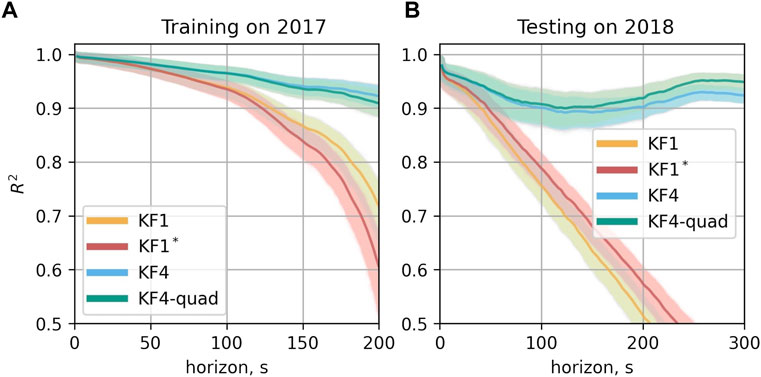
FIGURE 8. R²-score as a function of the forecast horizon. (A) On the training dataset, here from 2017 (B) on the test data from 2018. The mean value of R² is shown for each horizon in the darker color. The mean value was computed from 1,000 bootstrapped estimates of R², which are shown in the light color.

Predictions for selected fills 6,672, 6,674, 6,677, and 6,681 of the testing dataset of the year 2018 are shown in Figure 9 for the model (KF4). The values of input parameters in the training dataset lie in the interval (−1, 1). In Figure 9 one can see that the values of some of the input parameters for the testing dataset of 2018 which were standardized to the scale of the training dataset fall outside of interval (−1, 1). For the fills 6,672, 6,674, and 6,681 the scaled octupole current decreases from almost 2.5 to 1. It is visible that for these fills the model captured the dependence of the loss on the current correctly, even outside of the range of the values given during training.

FIGURE 9

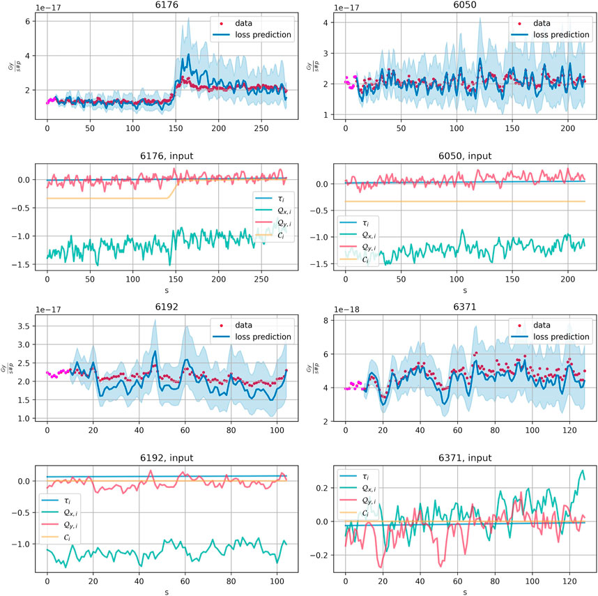
FIGURE 9. KF4 trained on the data of 2017, prediction on the fills 6176, 6050, 6192, and 6371 of 2018 and corresponding input control parameters. Pink points correspond to T₀ observations which the model uses to get initial KF smoother results. Further model propagates without seeing the loss and other output values, with control parameters given as the input. Two standard deviation confidence bands are shown in light blue.

Training on 2018: For the models estimated from the data of 2018, the results are shown in Figure 10. Remind, that the control parameters and their increments in the data of 2 years have different ranges. The results show that the case of modeling of the loss in 2017 based on the data of the year 2018 is more challenging for the proposed approach. Nevertheless KF4 and KF4-quad show significantly better predictive performance than (KF1), (KF1*). Selection of hyperparameters by optimizing MAE in cross-validation for KF4-quad did not lead to improvements compared to KF4. Predictions for the fills 6,176, 6,050, 6,192, and 6,371 of the year 2017 are shown in Figure 11 for KF4 model that was trained on the data of 2018.

FIGURE 10

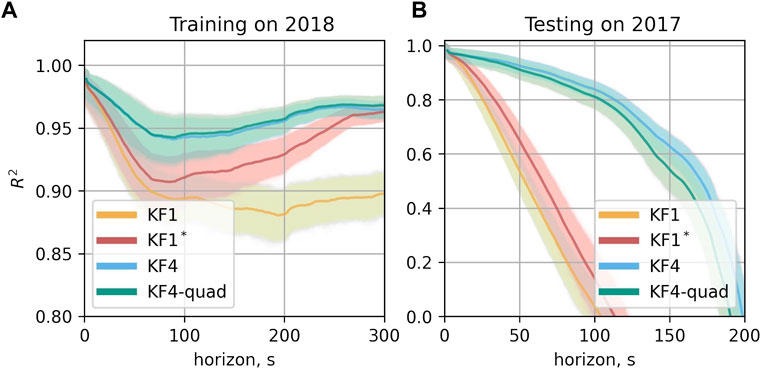
FIGURE 10. R²-score as a function of the forecast horizon. (A) On the training dataset, here from 2018 (B) on the test data in 2017.The mean value of R² is shown for each horizon in the darker color. The mean value was computed from 1,000 bootstrapped estimates of R², which are shown in the light color.

FIGURE 11

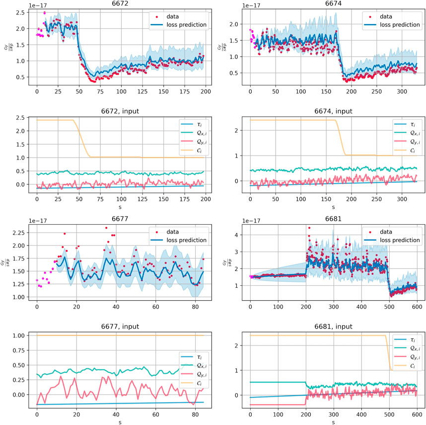
FIGURE 11. KF4 trained on the data of 2018, prediction on the fills 6726, 6674, 6677, and 6681 of 2018 and corresponding input control parameters. Pink points correspond to T₀ observations which the model uses to get initial KF smoother results. Further model propagates without seeing the loss and other output values, with control parameters given as the input. Two standard deviation confidence bands are shown in light blue.

3.2.1 Fitted models

KF4: Hyperparameter selection procedure from the data of 2017 led to the KF4 with the dimension of hidden process equal 16, which corresponds to the lag order 4 in the autoregressive part and MA parts of the VARMAX model. The selected input parameters increments history length was 80.

After checking that observability condition and condition on the initial value distribution (see remark in Section 2.2.1) for the estimated KF4 were satisfied, we could transform KF4 in the form of (9) to (8) to obtain the coefficients of equivalent VARMAX model formulation (3). Matrices with autoregressive coefficients are shown in Figure 12. One can see that for the losses $\mathcal{L}$, all output variables, including emittances and electron cloud induced heatloads, participate in AR terms. The opposite is not true, in the trained model, all the rest of output values have small coefficients corresponding to the lagged loss variables. Moving average coefficients in Figure 13 show that the first lag shocks have the most impact on the losses. The loss component of the output shares the shock of “0” lag with the other output variables. Further, instead of presenting coefficients for input variables and 80-lagged increments of input variables, we consider the impulse response function of the model.

FIGURE 12

FIGURE 12. Estimated autoregression matrices in KF4.

FIGURE 13

FIGURE 13. Estimated moving average part in KF4.

Impulse response functions: To analyze how the model (KF4) responds to shocks in one of the input variables, it is convenient to compute an Impulse Response Function (IRF) [20, 27]. Figure 14 demonstrates IRF for (KF4) trained on the data of 2017: the plot shows the change in output parameters after we modify the input parameters within the ranges in the training dataset. All the values of control and output values were set to median values based on the data from 2017, such that after standardizing them, their values equal zero. The impulse for each of the variables was taken as .5 of the range of the observations in 2017 at 50 s in Figure 14: for the horizontal tune ${\mathcal{Q}}_x$ the impulse was .005 from the level .272, for the vertical tune ${\mathcal{Q}}_y$ the impulse was .004 from .294, for octupole current the increase was 3.26A from 39.11A. After the value of the control variable increases, the model (KF4) continues to propagate until the outputs stabilize at a certain level. For emittances and electron cloud, IRFs demonstrate that the increase in the octupole current and tunes brings a more steady growth or decrease in values.

FIGURE 14

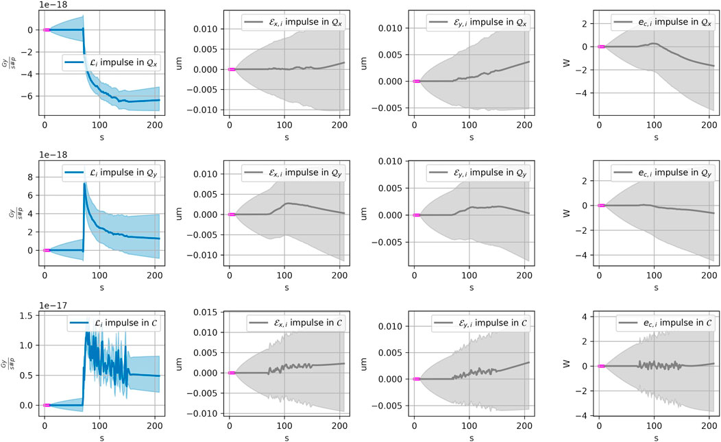
FIGURE 14. Impulse response plots for (KF4) model, impulses in the input parameters: in horizontal and vertical tunes and in the octupole current. The changes in losses and (2σ-)confidence intervals produced by (KF4) are shown in blue colors. The changes in the rest of the output components (horizontal and vertical emittances and electron cloud induced heatloads) and corresponding (2σ-)confidence intervals are shown in gray.

4 Conclusion

In this work, we proposed a VARMAX model to predict the evolution of the beam losses in the “PRERAMP” mode of the LHC on horizons up to 5 min based on control and context variables. Given the relationship with state-space models, the model is estimated under an equivalent Kalman Filter form. We considered a VARMAX models on the 1D loss time series and a VARMAX model with a vectorial output composed of the loss, the horizontal and vertical emittances and the aggregated heatload due to the electrom cloud as components, which induce the learning of a hidden state representation that helps predicting the evolution of the losses on a longer horizon. In addition, we proposed an extension of the linear KF for the transition matrix and exogeneous coefficients dependent on the input variables.

The hyperparameter selection procedure on lags needed in the exogeneous and in the autoregressive terms revealed that the control variables have lagged effects on the losses with lags of up to 80 s while a shorter history of 4 s is needed for the autoregressive term, to obtain good predictions on a horizon of 5 min. The loss model with additional output components fitted on the data from 2017 performed well in predicting the loss measured at IR7 in 2018 for a horizon of up to 5 min.

The inclusion of additional output variables in the model, such as heatload and emittance, helped significantly to improve the long-term prediction of the loss. Finally, in terms of interpretability of the model, the proposed impulse response analysis of the estimated model can help investigate different scenarios of the changes in the control parameters to understand their effect on the loss.

A possible extension of this work could be to model jointly both beam losses, which might account for beam coupling. Further, the development of a tool that could guide the operators in the control room could be anticipated, which would propose optimal changes in the available parameters space for a given set of initial setting (i.e. emittances, intensities, etc.) while commissioning and re-optimizing the collider at every physics fill. Besides that, the new data obtained from the operation should be useful to re-train and revise the model. Our model based on machine data is a valuable addition to numerical models of particle losses, that can boost and improve the understanding of particle losses and help in the design of future colliders.

Data availability statement

The datasets analyzed in this study are publicly available. This data can be found here: https://doi.org/10.5281/zenodo.7305102.

Author contributions

EK, GO, MS, LC, and TP contributed to the conception and design of the approach. EK performed the statistical analysis and wrote the first draft of the manuscript. All authors contributed to manuscript revision, read, and approved the submitted version.

Funding

This work is funded by the Swiss Data Science Center project grant C18-07. This work was performed under the auspices and with the support from the Swiss Accelerator Research and Technology (CHART) program. Open access funding provided by ETH Zurich.

Conflict of interest

The authors declare that the research was conducted in the absence of any commercial or financial relationships that could be construed as a potential conflict of interest.

The reviewer EF declared a shared affiliation with the author MS to the handling editor at the time of review.

Publisher’s note

All claims expressed in this article are solely those of the authors and do not necessarily represent those of their affiliated organizations, or those of the publisher, the editors and the reviewers. Any product that may be evaluated in this article, or claim that may be made by its manufacturer, is not guaranteed or endorsed by the publisher.

Supplementary material

The Supplementary Material for this article can be found online at: https://www.frontiersin.org/articles/10.3389/fphy.2022.960963/full#supplementary-material

Footnotes

¹“Fill” refers to the time period starting from injection of new beam into the LHC until the beam gets dumped. The filling scheme, on the other hand, defines which of the radio-frequency buckets are filled with particles and which ones are left empty.

References

1. Coyle LTD. Machine learning applications for hadron colliders: LHC lifetime optimization. Switzerland: Grenoble INP, France and EPFL (2018).

Google Scholar

2. Evans L. The large hadron collider. New J Phys (2007) 9:335. doi:10.1088/1367-2630/9/9/335

CrossRef Full Text | Google Scholar

3. Brüning O, Burkhardt H, Myers S. The large hadron collider. Prog Part Nucl Phys (2012) 67:705–34. doi:10.1016/j.ppnp.2012.03.001

CrossRef Full Text | Google Scholar

4. Arpaia P, Azzopardi G, Blanc F, Bregliozzi G, Buffat X, Coyle L, et al. Machine learning for beam dynamics studies at the cern large hadron collider. Nucl Instr Methods Phys Res Section A: Acc Spectrometers, Detectors Associated Equipment (2021) 985:164652. doi:10.1016/j.nima.2020.164652

CrossRef Full Text | Google Scholar

5. Li S, Zacharias M, Snuverink J, Coello de Portugal J, Perez-Cruz F, Reggiani D, et al. A novel approach for classification and forecasting of time series in particle accelerators. Information (2021) 12:121. doi:10.3390/info12030121

CrossRef Full Text | Google Scholar

6. Koser D, Waites L, Winklehner D, Frey M, Adelmann A, Conrad J. Input beam matching and beam dynamics design optimizations of the IsoDAR RFQ using statistical and machine learning techniques. Front Phys (2022) 10:302. doi:10.3389/fphy.2022.875889

CrossRef Full Text | Google Scholar

7. Schenk M, Coyle L, Pieloni T, Obozinski G, Giovannozzi M, Mereghetti A, et al. Modeling particle stability plots for accelerator optimization using adaptive sampling JACoW IPAC (2021), 1923–1926. doi:10.18429/JACoW-IPAC2021-TUPAB216

CrossRef Full Text | Google Scholar

8. Edelen A, Neveu N, Frey M, Huber Y, Mayes C, Adelmann A. Machine learning for orders of magnitude speedup in multiobjective optimization of particle accelerator systems. Phys Rev Accel Beams (2020) 23:044601. doi:10.1103/physrevaccelbeams.23.044601

CrossRef Full Text | Google Scholar

9. Coyle L, Blanc F, Pieloni T, Schenk M, Buffat X, Camillocci M, et al. Detection and classification of collective beam behaviour in the LHC. JACoW IPAC (2021), 4318–21. doi:10.18429/JACoW-IPAC2021-THPAB260

CrossRef Full Text | Google Scholar

10. Abada A, Abbrescia M, AbdusSalam SS, Abdyukhanov I, Abelleira Fernandez J, Abramov A, et al. FCC-hh: The hadron collider. Phys J Spec Top (2019) 228:755. doi:10.1140/epjst/e2019-900087-0

CrossRef Full Text | Google Scholar

11. Abada A, Abbrescia M, AbdusSalam SS, Abdyukhanov I, Abelleira Fernandez J, Abramov A, et al. HE-LHC: The high-energy large hadron collider. Phys J Spec Top (2019) 228:1109. doi:10.1140/epjst/e2019-900088-6

CrossRef Full Text | Google Scholar

12. Hermes PD, Redaelli S, Jowett J, Bruce R. Betatron cleaning for heavy ion beams with IR7 dispersion suppressor collimators. In: 6th International Particle Accelerator Conference; Richmond, VA (2015). No. CERN-ACC-2015-0193.

Google Scholar

13. Zimmermann F. Electron cloud effects in the LHC. Geneva: Proceedings ECLOUD (2002). doi:10.5170/CERN-2002-001.47

CrossRef Full Text | Google Scholar

14. Edwards DA, Syphers MJ. An introduction to the physics of high energy accelerators. John Wiley & Sons (2008).

Google Scholar

15. Zimmermann F. A simulation study of electron-cloud instability and beam-induced multipacting in the LHC. LHC Project Report 95, CERN (1997), 18.

CrossRef Full Text | Google Scholar

16. Aquilina N, Giovannozzi M, Lamont M, Sammut N, Steinhagen R, Todesco E, et al. Tune variations in the large hadron collider. Nucl Instr Methods Phys Res Section A: Acc Spectrometers, Detectors Associated Equipment (2015) 778:6–13. doi:10.1016/j.nima.2014.12.081

CrossRef Full Text | Google Scholar

17. Krymova E, Obozinski G, Schenk M, Coyle LT, Pieloni T. Data-driven modeling of beam loss in the lhc (2022). doi:10.5281/zenodo.7305102

CrossRef Full Text | Google Scholar

18. Fokianos K, Rahbek A, Tjøstheim D. Poisson autoregression. J Am Stat Assoc (2009) 104:1430–9. doi:10.1198/jasa.2009.tm08270

CrossRef Full Text | Google Scholar

19. Solfaroli Camillocci M, Lamont M, Juchno M, Schaumann M, Wenninger J, Todesco E. Feed-forward corrections for tune and chromaticity injection decay during 2015 lhc operation. In: Proceedings of IPAC2016; Busan, Korea (2016), 1489–1492.

Google Scholar

20. Hamilton JD. Time series analysis. Princeton, NJ: Princeton university press (2020).

Google Scholar

21. de Jong P, Penzer J. The ARMA model in state space form. Stat Probab Lett (2004) 70:119–25. doi:10.1016/j.spl.2004.08.006

CrossRef Full Text | Google Scholar

22. Casals J, Sotoca S, Jerez M. A fast and stable method to compute the likelihood of time invariant state-space models. Econ Lett (1999) 65:329–37. doi:10.1016/s0165-1765(99)00165-2

CrossRef Full Text | Google Scholar

23. Casals J, García-Hiernaux A, Jerez M. From general state-space to VARMAX models. Mathematics Comput Simulation (2012) 82:924–36. doi:10.1016/j.matcom.2012.01.001

CrossRef Full Text | Google Scholar

24. Abernethy J, Bach F, Evgeniou T, Vert JP. A new approach to collaborative filtering: Operator estimation with spectral regularization. J Machine Learn Res (2009) 10: 803–826.

Google Scholar

25. Hou K, Zhou Z, So AMC, Luo ZQ. On the linear convergence of the proximal gradient method for trace norm regularization. Adv Neural Inf Process Syst (2013) 26: 1–9.

Google Scholar

26. Ohtani K. Bootstrapping r2 and adjusted r2 in regression analysis. Econ Model (2000) 17:473–83. doi:10.1016/s0264-9993(99)00034-6

CrossRef Full Text | Google Scholar

27. Belomestny D, Krymova E, Polbin A. Bayesian tvp-varx models with time invariant long-run multipliers. Econ Model (2021) 101:105531. doi:10.1016/j.econmod.2021.105531

CrossRef Full Text | Google Scholar