On the hardness of quadratic unconstrained binary optimization problems

We use exact enumeration to characterize the solutions of quadratic unconstrained binary optimization problems of less than 21 variables in terms of their distributions of Hamming distances to close-by solutions. We also perform experiments with the D-Wave Advantage 5.1 quantum annealer, solving many instances of up to 170-variable, quadratic unconstrained binary optimization problems. Our results demonstrate that the exponents characterizing the success probability of a D-Wave annealer to solve a quadratic unconstrained binary optimization correlate very well with the predictions based on the Hamming distance distributions computed for small problem instances.

1 Introduction

Optimization is at the heart of problem solving in science, engineering, finance, operational research etc. The basic idea is to associate a cost with each of the possible values of the variables that describe the problem and try to minimize this cost. Of particular importance is the class of so-called discrete optimization problems in which some or all the variables take values from a finite set of possibilities. Discrete optimization problems are often NP-hard [1] which, in practice and in simple terms, means that solving such a problem on a digital computer will require resources that increase exponentially with the number of variables.

Many discrete optimization problems can be reformulated as quadratic unconstrained binary optimization (QUBO) problems [2, 3]. Solving a QUBO amounts to finding the values of the N binary variables x_i = 0, 1 that minimize the cost function

$\text{Cost}\left(x_1,\dots ,x_N\right)=\sum _{1=i\le j=N}{Q}_{i,j}{x}_i{x}_j,x_i=\mathrm{0,1},(1)$

where Q_i,j = Q_j,i is a symmetric N × N matrix of floating point numbers.

The interest in expressing discrete optimization problems in the form of QUBOs has recently gained momentum by the development of quantum annealers manufactured by D-Wave systems [4, 5]. In theory [6], quantum annealers make use of the adiabatic theorem [7] to find the ground state of the Ising model defined by the Hamiltonian

$H=\sum _{1=i<j=N}{J}_{i,j}{S}_i{S}_j+\sum _{i=1}^N{h}_i{S}_i,(2)$

Substituting S_i = 1 − 2x_i = ±1 in Eq. 2 yields

$H=\text{Cost}\left(x_1,\dots ,x_N\right)-C_0,(3)$

where the relations between the Q’s in Eq. 1 and J’s, h′s, and C₀ in Eqs 2 and 3 are given in Appendix A.

Obviously, the transformation S_i = 1 − 2x_i = ±1 does not change the nature of the optimization problem. In other words, minimizing the cost function of a QUBO Eq. 1 or finding the ground state of the Ising model Eq. 2 are equally difficult. Currently available quantum annealer hardware often finds ground states of Eq. 2 for fully-connected problems with about 200 variables or less in about micro seconds [4, 5], which is quite fast, suggesting that as larger quantum annealers become available, they have the potential to solve large QUBOs in a relatively short real time.

Although the transformation S_i = 1 − 2x_i = ±1 does not change the nature of the optimization problem, the formulation of a particular optimization problem in terms of a QUBO can. For instance, 2-satisfiability problems (2SAT) [1] (see Section 2.1) can be solved with computational resources that increase linearly with the number of binary variables [8–10]. However, the special features of 2SAT-problem that permits its efficient solution are lost when it is expressed as a QUBO/Ising model. In fact, the equivalent QUBO becomes notoriously hard to solve by e.g., simulated annealing [11]. On the other hand, it is also not difficult to construct Ising models of which the ground state is very easy to find.

In view of the potential of quantum annealers for solving large QUBOs in the near future, it is of interest to gain some insight into the degree of success by which a quantum annealer is expected to solve a QUBO/finding the ground state of corresponding Ising model, without actually performing the experiment.

In this paper, we show, using three classes of problems, that the following two factors are well correlated:

1. The success probability a D-Wave annealer finds the ground state of the Ising model/solves the QUBO.

2. The distribution of Hamming distances between the ground state and the lowest excited states computed for relatively small, representative problem instances.

We demonstrate that the differences between the Hamming distance distributions are correlated with the size-dependent scaling of the success probabilities with which D-Wave quantum annealers find the ground state.

The structure of the paper is as follows. Section 2 introduces the three different classes of QUBO problems that we analyze. In section 3, we briefly review the three different methods by which we solve the QUBO instances. Section 4 and Section 5 present and discuss our results for the Hamming distance and level spacing distributions, and quantum annealing experiments, respectively. In Section 4, we summarize our findings.

2 Quadratic unconstrained binary optimization problems

2.1 2-Satisfiability problems

The problem of assigning values to binary variables such that given constraints on pairs of variables are satisfied is called 2-satisfiability [1]. 2SAT is a special case of the general Boolean satisfiability problem, involving constraints on more than two variables. In contrast to e.g. 3SAT which is known to be NP-complete, 2SAT can be solved in polynomial time. The most efficient algorithms solve 2SAT in a time which is proportional to the number of variables [8–10].

A 2SAT problem is specified by N binary variables x_i = 0, 1 and a conjunction of M clauses defining a binary-valued cost function

$\begin{array}{ccc}\hfill C& =\hfill & C\left(x_1,\dots ,x_N\right)\hfill \\ \hfill & =\hfill & \left(L_{\mathrm{1,1}}\vee L_{\mathrm{1,2}}\right)\wedge \left(L_{\mathrm{2,1}}\vee L_{\mathrm{2,2}}\right)\wedge \dots \wedge \left(L_{M,1}\vee L_{M,2}\right),\hfill \end{array}(4)$

where the literal L_α,j stands for either x_i(α,j) or its negation ${\bar{x}}_{i(\alpha ,j)}$, for α = 1, … , M and j = 1, 2. The function i (α, j) maps the pair of indices (α, j) onto the index i of the binary variable x_i. A 2SAT problem is satisfiable if one can find at least one assignment of the x_i’s which makes the cost function C true.

Solving a 2SAT problem is equivalent to finding the ground state of the Ising-spin Hamiltonian [2, 11, 12].

$H_{2\text{SAT}}=\sum _{\alpha =1}^M{h}_{2\text{SAT}}\left({\epsilon }_{\alpha ,1}{S}_{i\left(\alpha ,1\right)},{\epsilon }_{\alpha ,2}{S}_{i\left(\alpha ,2\right)}\right),(5)$

where ɛ_α,j = +1 (−1) if L_α,j stands for $x_i({\bar{x}}_i)$ and

$h_{2\text{SAT}}\left(S_l,S_m\right)=\left(S_l-1\right)\left(S_m-1\right),S_m,S_l=\pm 1.(6)$

Grouping and rearranging terms, Eq. 5 reads

$H_{2\text{SAT}}=\sum _{1\le i<j\le N}{J}_{i,j}{S}_i{S}_j+\sum _{i=1}^N{h}_i{S}_i+C_1,(7)$

where C₁ is an irrelevant constant. Therefore, solving a 2SAT problem Eq. 4 is equivalent to solving the QUBO problem defined by Eq. 7. It may be of interest to mention that if one is given a QUBO problem without knowing that it originated from a 2SAT problem, it is not clear that the QUBO can be solved in a time linear in N.

Constructing 2SAT problems is easy but finding 2SAT problems that have a unique known ground state and a highly degenerate first-excited state quickly becomes more difficult with increasing N [11]. We have generated 15 sets of 2SAT problems that have a unique known ground state and a highly degenerate first-excited state, each set corresponding to an N, with N ranging from 6 to 20 with the number of clauses M = N + 1. The graphs representing these problems are not fully connected, that is not all J_i,j’s are different from zero. For our sets of 2SAT problems, the h_i’s and J_i,j’s can take the integer values between −2 and 2.

2.2 Fully-connected spin glass

The spin glass model is defined by the Hamiltonian Eq. 2. Computing the ground state configuration of the spin glass problem is, in general, very hard and is proven to be NP-hard [13]. To verify that a spin configuration has the lowest energy, one would (in general) have to go through all the 2^N − 1 other configurations to check if it indeed has the lowest energy. The qualifier “in general” is important here for there are cases, such when all J_i,j = 0, for which the ground state is trivial to find. To effectively rule out such trivially solvable problems, we use uniform (pseudo) random numbers in the range [− 1, 1] to assign values to all the J_i,j’s and all the h_i’s. The probability that one of the J_i,j’s is zero is extremely small, justifying the term “fully-connected spin glass”. In the following, we refer to the set of model instances generated in this manner as RAN problems.

2.3 Fully-connected regular spin-glass model

In the course of developing an QUBO-based application to benchmark large clusters of GPUs (see Appendix B), we discovered by accident that the ground state of the spin glass defined by Eq. 2 with

$\begin{array}{ccc}\hfill J_{i,j}& =\hfill & 1-\left(i+j-2\right)/\left(N-1\right),i\ne j,\hfill \\ \hfill h_i& =\hfill & 1-2\left(i-1\right)/\left(N-1\right),\hfill \end{array}(8)$

seems to have a peculiar structure. Note that of the order of N J_i,j’s are zero.

Although we have not been able to give a proof valid for all N, up to N = 200 we have not found any counter example for conjecture that the ground states of the Ising model with parameters given by Eq. 8 is given by (S₁ = −1, … , S_k = −1, S_k+1 = 1, … , S_N = 1) or, equivalently (x₁ = 1, … , x_k = 1, x_k+1 = 0, … , x_N = 0) where k is the integer that minimizes

$f\left(k\right)=\sum _{1\le i\le j\le k}{Q}_{i,j}=\frac{k\left(N-k\right)\left(N-2k+2\right)}{N-1}.(9)$

Thus, although we are solving a fully connected QUBO problem, if our conjecture is correct, its solution is very easy to find for any N. We refer to the special, fully-connected regular spin glass problems defined by Eq. 8 as REG problems.

From Eq. (2), it immediately follows that randomly reversing a spin i and replacing h_j by −h_j and J_i,j by −J_i,j for all j does not change the ground state energy of a QUBO problem. Applying such “gauge transformation” to sets of randomly selected spins generated a set of REG problems that are mathematically equivalent. This feature, in combination with the fact that the ground state is known (for at least N ≤ 200) makes REG problems well-suited for testing and benchmarking purposes, of both conventional and quantum hardware.

3 Methods for solving QUBOs

We solve QUBOs using three different methods.

1. A computer code referred to as QUBO22 which uses GPUs and/or CPUs to solve QUBOs, Polynomial Unconstrained Binary Optimization (PUBOs), and Exact Cover problems (reformulated as QUBOs). QUBO22 simply enumerates all 2^N possible values of the binary variables x₁, … , x_N while keeping track of those configurations of x’s that yield the lowest, next to lowest and largest cost. QUBO22 obviously always finds the true ground state. The number of arithmetic operations required to solve a QUBO is proportional to N(N − 1)2^N. With the supercomputers that are available to us, the exponential increase with N limits the application QUBO22 to problems of size N ≤ 58.In order to compute the Hamming distance between excited states and the ground state and level spacing distributions, it is necessary to keep track of a large number of different states. To this end, we use another code, also based on full enumeration, which in practice, can readily handle problems up to N = 20.

2. Heuristic methods can solve QUBOs in (much) less time than QUBO22 can. However, heuristic methods do not guarantee to return the solution of the QUBO problem (although they very often do). In our work, we use qbsolv, a heuristic solver provided by D-Wave, to compute the ground states of all problem instances. For those problems which QUBO22 can solve, the ground states obtained by qbsolv and QUBO22 match. For all RAN and REG problems up to N = 200, the ground states obtained by qbsolv and the D-Wave Advantage 4.1 Hybrid solver are also the same.

3. We have used the D-Wave Advantage 5.1 quantum annealer to solve all problem instances. We calculate the success probabilities by using the ground states obtained by qbsolv. Note that in no case could the D-Wave annealer find states with lower energies than that obtained from qbsolv. The data for the success probabilities is then used to analyse the scaling behavior as a function of the problem size N.

It should be noted that the ground states of the large problems (N > 58) belonging to the REG and the RAN class are obtained heuristically by qbsolv and D-Wave Hybrid solver in this work. In principle, the states obtained in such a way might not be the true ground states, but for the size of the problems considered here (N < 200), that is unlikely to be the case.

4 Hamming distance and level spacing

The Hamming distance between two bitstrings (or strings of S’s) of equal length is defined as the number of positions at which the corresponding bits (S’s) are different. For each of the problems in our set, we use exact enumeration to find at most 6,037 states with the lowest energies. With this data we compute the Hamming distances between the ground state and these excited states.

In this section, we only present results for one representative N = 20 problem taken from the 2SAT, RAN and REG class, respectively. The plots for other N = 20 instances look similar, and the corresponding average Hamming distance distributions are given in Appendix C.

From Figure 1 we draw the following conclusions. Recall that the first excited states used to generate Figure 1A all have the same energy. By construction, according to Eq. 6, the level spacing distribution Figure 1B is nonzero for Δ = 4 only. Now imagine that the search process (in e.g., simulated annealing) for the ground state ends up in one of these excited states. From Figure 1A it then follows immediately that the probability to reach the ground state by single-spin flipping will be very low. Indeed, most of these excited states have a Hamming distance 10–15 and it would require a miracle to have a particular sequence of single-spin flips reducing the Hamming distance to zero. In summary, from Figure 1 it is easy to understand why this particular class of 2SAT problems is very hard to solve by simulated annealing [11, 12].

FIGURE 1

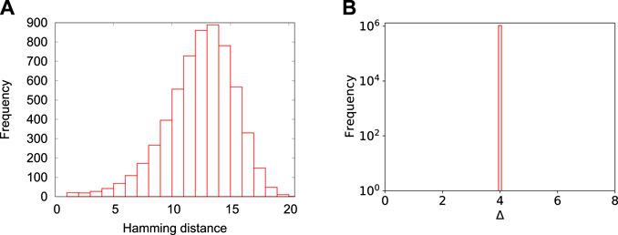
FIGURE 1. (color online) (A) Frequencies of Hamming distances between the ground state configuration and the first 6,036 excited states, obtained by analyzing a N = 20 2SAT problem. (B) Level spacing distribution, that is the distribution of the energy difference Δ between the first excited state and the ground state, the second excited state and the first excited state, etc. For the 2SAT problem considered, the first 6,036 excited state are degenerate, yielding one peak at Δ = 4.

From Figure 2 we conclude the following. In contrast to Figure 1A, most of the weight of the Hamming distance distribution is centered around five. Also the level spacing distribution Figure 2B is very different from that of the 2SAT problems. This suggests that five or less spin flips may suffice to change the excited state into the ground state. Thus, in comparison with the class of 2SAT problems that we have selected, the RAN problems are expected to be much more amenable to simulated and quantum annealing.

FIGURE 2

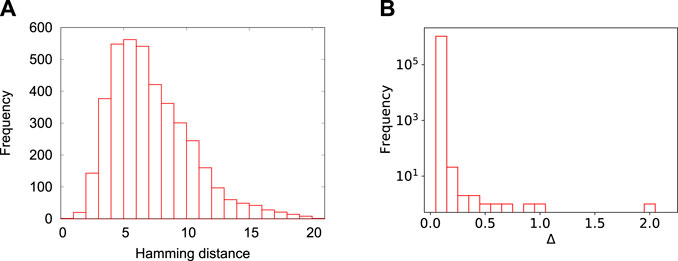
FIGURE 2. (color online) Same as Figure 1 except that the problem instance belongs to the class of N = 20 RAN problems and that we only show the results for the 4,000 states which are closest to the ground state in energy. In this case, the first 4,000 excited energy levels differ by approximately 17 units whereas for 2SAT, the energy of 6,036 of the lowest excited states are only 4 units of energy higher than the ground state.

The Hamming distance and level spacing distribution of a REG problem (see Figure 3) are very different from the corresponding ones of the 2SAT or RAN problems. There are only five distinct energy level spacings for these problems and the Hamming distance distribution shows that many of the excited states differ from the ground state by only a few spin flips. Therefore, we may expect that of the three classes of problems considered, problems of the REG class are the least difficult to solve by simulated or quantum annealing.

FIGURE 3

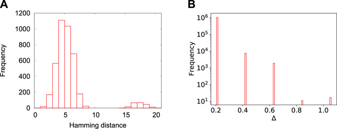
FIGURE 3. (color online) Same as Figure 1 except that the problem instance belongs to the class of N = 20 REG problems. There are only five distinct energy differences in this case. The energies of the 4,000 lowest energy levels differ by approximately 24 units.

5 Quantum annealing experiments

We demonstrate that the conclusions of Section 4, drawn from the analysis of small problem instances, correlate very well with the degree of difficulty observed when solving significantly larger problems on a D-Wave Advantage 5.1 quantum annealer.

In Figure 4A we present the results obtained by solving all REG-class problems on a D-Wave quantum annealer. For each N, instances were generated by spin-reversal transformations, as explained above. As the problem size N increases, the success probability, that is the relative frequency with which the D-Wave yields the ground state, decreases exponentially, from $\mathcal{O}(1)$ to $\mathcal{O}(10^{-6})$. Fitting exponentials to the data reveals that the exponent changes from −0.039 to −0.090 at about N = 80. The larger the absolute value of the exponent, the more difficult it is to solve the QUBO by quantum annealing. Since using brute-force search, the success probability scales as 2^−N, we believe that in the asymptotic limit, the success probability using quantum annealing should scale similarly at worst, except for a different prefactor. Therefore, we use exponential functions linear in N as the fitting functions for the scaling of the success probability. Other alternatives for the fitting functions are considered in Appendix D.

FIGURE 4

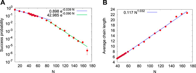
FIGURE 4. (color online) (A) Mean success probability and its variance as a function of the problem size N, obtained by solving all problem instances of the REG class on a D-Wave Advantage 5.1 quantum annealer. Solid lines are least square fits to data for N < 80 and N > 80, respectively. (B) Average chain length as a function of the problem size N, a measure for the average number of physical qubits that is required to represent one variable in the QUBO problem.

With increasing problem size N, it becomes more difficult and eventually impossible to map the fully-connected QUBO problem onto the Chimera or Pegasus lattice that defines the connectivity of the D-Wave qubits. To embed even a small fully-connected problem onto the working graph of the system, two or more physical qubits are chained together by means of the relative chain strength parameter, to represent a logical qubit of the original problem. For instance, a N = 170 variable REG problem maps onto about 3,964 physical qubits of a D-Wave Advantage 5.1. We quantify this aspect by computing the average chain length, a measure for the average number of physical qubits that the D-Wave software uses to map a variable onto a group of physical qubits. Figure 4B shows the average chain length, computed from data obtained by solving all REG problems. Clearly, the average chain length only increases linearly with N and does not show any sign of the crossover observed in the scaling dependence of the success probabilities, seen in Figure 4A. Furthermore, the chain break fraction which, as the name suggests, is the fraction of chains that are broken in the sample, remains zero for even the larger problems belonging to the set. Thus, the embedding of the problem on the D-Wave lattice cannot be held responsible for the crossover in the scaling of the success probability.

In Figure 5 we present the results obtained by solving all RAN-class problems on a D-Wave quantum annealer. At first glance, Figures 4, 5 may look similar but there are significant differences. First note that there is no data point for N = 90 simply because after 200,000 attempts, the D-Wave did not return the ground state. For N = 100, we were more lucky but for N ≥ 110 we were not, in sharp contrast with the case of REG problems for which the D-Wave Advantage 5.1 returned the correct solutions up to N = 170. Clearly, the D-Wave Advantage 5.1 quantum annealer finds RAN problems more difficult to solve than REG problems, although both their QUBOs involve fully connected graphs. This observation is further confirmed by fitting exponentials to the data. As in the REG case, there is a crossover, not at N = 80 but at N ≈ 35, with the exponent changing from −0.102 to −0.162, see Figure 5A.

FIGURE 5

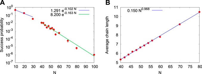
FIGURE 5. (color online) Same as Panel 5 except that the problem instances belongs to the RAN class.

The class of 2SAT problems analyzed in this paper has already been studied extensively through computer simulated quantum annealing and by means of D-Wave quantum annealers [14, 15]. The general conclusion is that, in spite of the small number (N ≤ 20) of variables, the 2SAT class contains instances which are very difficult to solve by simulated annealing [11] and quantum annealing [14, 15]. For completeness, in Figure 6 we present data for the success probabilities for the set of N ≤ 20 problems, also used to study the Hamming distance and level spacing distributions. Focusing on problem of size N = 14, … , 20, we find that the success probabilities, obtained by the D-Wave Advantage 5.1 quantum annealer, decrease exponentially with an exponent of −0.269, considerable larger in absolute value than the exponents −0.162 and −0.090 of the corresponding RAN and REG problems, respectively. Of course, we cannot simply extrapolate the 14 ≤ N ≤ 20 exponent to larger N’s but, we believe it is unlikely that this exponent will become smaller as N increases further.

FIGURE 6

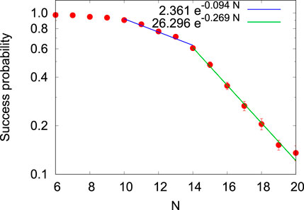
FIGURE 6. (color online) Same as Figure 4A except that the problem instances belongs to the 2SAT class.

For our D-Wave experiments, we used the default annealing time of 20 μs. One may expect that by using longer annealing times, the success probabilities will increase and more and larger RAN class problems can be solved.

6 Conclusion

We have analyzed a large number of QUBOs that we have synthesized in three different ways. The first set of QUBOs was obtained by mapping a special selection of 2SAT problems onto QUBOs. These 2SAT problems are special in the sense that they possess a unique ground state and a large number of degenerate, first excited states. Findings such 2SAT problems is computationally demanding, limiting our search to instances with less than 21 variables.

The second set of problems contains Ising models in which uniform random numbers determine all the two-spin interactions and all the local fields. From a statistical mechanics point of view, such fully-connected spin-glass models exhibit frustration and computing their ground states and temperature dependent properties is known to be difficult.

Finally, the third set of problems is also of the fully-connected spin-glass type but the interaction and field values are given by a peculiar linear function of the spin indices. Our numerical experiments suggest that this problem may be solvable for any number of spins but we have not yet been able to proof this conjecture mathematically.

We have calculated Hamming distance distributions and level spacing distributions for small problem instances and also submitted the small and large QUBO instances to a D-Wave quantum annealer. Our results demonstrate that the exponents characterizing the success probability of a D-Wave annealer to solve a QUBO correlate very well with the predictions based on the Hamming distance and level spacing distributions computed for small QUBO instances.

Since for the 2SAT problems, in order to reach the ground state from one of the first excited states one would need to flip exactly the same number of bits as the Hamming distance between them, these problems should be difficult to solve using classical algorithms like simulated annealing. This has found to be the case for these problems [12]. On the other hand, not only does the peak of the Hamming distance distributions in case of the REG and RAN problems correspond to a smaller number, meaning a smaller number of single bit-flip operations to reach the ground state from one of the low-lying energy states, the presence of many energy levels between the ground state and the lowest 4,000 excited states should make these problems easier for the classical algorithms. It will therefore be of interest to use simulated annealing for solving the three sets of problems and to study if the Hamming distance distributions for small problem instances also predict the effectiveness of simulated annealing in the future.

Data availability statement

The datasets presented in this study can be found in online repositories. The names of the repository/repositories and accession number(s) can be found below: https://jugit.fz-juelich.de/qip/qubo-problems.

Author contributions

All authors contributed to the conception and design of the research. VM performed the experiments and analyzed the results. HDR prepared the first draft of the manuscript. All authors participated in revising and correcting the manuscript.

Acknowledgments

The authors gratefully acknowledge support from the project JUNIQ which has received funding from the German Federal Ministry of Education and Research (BMBF) and the Ministry of Culture and Science of the State of North Rhine-Westphalia and from the Gauss Centre for Supercomputing eV (www.gauss-centre.eu) for funding this project by providing computing time on the GCS Supercomputer JUWELS at Jülich Supercomputing Centre (JSC).

Conflict of interest

The authors declare that the research was conducted in the absence of any commercial or financial relationships that could be construed as a potential conflict of interest.

Publisher’s note

All claims expressed in this article are solely those of the authors and do not necessarily represent those of their affiliated organizations, or those of the publisher, the editors and the reviewers. Any product that may be evaluated in this article, or claim that may be made by its manufacturer, is not guaranteed or endorsed by the publisher.

References

1. Garey GR, Johnson D. Computers and intractability. New York, NY, USA: W.H. Freeaman (2000).

Google Scholar

2. Lucas A. Ising formulations of many NP problems. Front Phys (2014) 2:5. doi:10.3389/fphy.2014.00005

CrossRef Full Text | Google Scholar

3. Lewis M, Glover F. Quadratic unconstrained binary optimization problem preprocessing: Theory and empirical analysis. arXiv:cs.AI/1705.09844 (2017).

CrossRef Full Text | Google Scholar

4. Johnson MW, Amin MHS, Gildert S, Lanting T, Hamze F, Dickson N, et al. Quantum annealing with manufactured spins. Nature (2011) 473:194–8. doi:10.1038/nature10012

PubMed Abstract | CrossRef Full Text | Google Scholar

5. McGeoch C, Farré P. The D-wave advantage system: An overview. In: Tech. Rep. Burnaby, BC, Canada: D-Wave Systems Inc (2020). D-Wave Technical Report Series 14-1049A-A.

Google Scholar

6. Kadowaki T, Nishimori H. Quantum annealing in the transverse ising model. Phys Rev E (1998) 58:5355–63. doi:10.1103/physreve.58.5355

CrossRef Full Text | Google Scholar

7. Born M, Fock V. Beweis des adiabatensatzes. Z Physik (1928) 51:165–80. doi:10.1007/bf01343193

CrossRef Full Text | Google Scholar

8. Krom MR. The decision problem for a class of first-order formulas in which all disjunctions are binary. MLQ - Math Log Quart (1967) 13:15–20. doi:10.1002/malq.19670130104

CrossRef Full Text | Google Scholar

9. Even S, Itai A, Shamir A. On the complexity of timetable and multicommodity flow problems. SIAM J Comput (1976) 5:691–703. doi:10.1137/0205048

CrossRef Full Text | Google Scholar

10. Aspvall B, Plass MF, Tarjan RE. A linear-time algorithm for testing the truth of certain quantified boolean formulas. Inf Process Lett (1979) 8:195. doi:10.1016/0020-0190(82)90036-9

CrossRef Full Text | Google Scholar

11. Neuhaus T. Monte Carlo search for very hard K-SAT realizations for use in quantum annealing. arXiv:1412.5361 (2014).

Google Scholar

12. Neuhaus T. Quantum searches in a hard 2-SAT ensemble. arXiv:1412.5460 (2014).

Google Scholar

13. Barahona F. On the computational complexity of ising spin glass models. J Phys A: Math Gen (1982) 15:3241–53. doi:10.1088/0305-4470/15/10/028

CrossRef Full Text | Google Scholar

14. Mehta V, Jin F, De Raedt H, Michielsen K. Quantum annealing with trigger Hamiltonians: Application to 2- satisfiability and nonstoquastic problems. Phys Rev A (Coll Park) (2021) 104:032421. doi:10.1103/physreva.104.032421

CrossRef Full Text | Google Scholar

15. Mehta V, Jin F, De Raedt H, Michielsen K. Quantum annealing for hard 2-SAT problems : Distribution and scaling of minimum energy gap and success probability. arXiv:2202.00118 (2022).

Google Scholar

16. Alvarez D. JUWELS cluster and booster: Exascale pathfinder with modular supercomputing architecture at juelich supercomputing Centre. J large-scale Res Facil JLSRF (2021) 7:A183. doi:10.17815/jlsrf-7-183

CrossRef Full Text | Google Scholar

Appendix A: Relation between QUBOs and ising models

The relations between the Q_i,j’s, J_i,j’s, h_i’s and C₀ are given by

$J_{i,j}=\frac{1}{4}{Q}_{i,j}\text{if}i\ne j,J_{i,i}=0,(\mathrm{A1})$

$h_i=-\frac{1}{2}\left(Q_{i,i}+\frac{1}{2}\sum _{j\ne i}{Q}_{i,j}\right),(\mathrm{A2})$

$\begin{array}{ccc}\hfill C_0& =\hfill & \frac{1}{2}\sum _{i=1}^N{Q}_{i,i}+\frac{1}{4}\sum _{1\le i<j\le N}{Q}_{i,j}\hfill \\ \hfill & =\hfill & \sum _{1\le i<j\le N}{J}_{i,j}-\sum _{i=1}^N\left[h_i+\sum _{j\ne i}{J}_{i,j}\right],\hfill \end{array}(\mathrm{A3})$

$Q_{i,j}=4J_{i,j}-2{\delta }_{i,j}\left(h_i+\sum _{k\ne i}{J}_{i,k}\right).(\mathrm{A4})$

Appendix B: Exact QUBO solver

We briefly discuss the scaling behavior the QUBO solver QUBO22 with the problem size N and also give an impression of the resources that are required to solve QUBO problems exactly. Not only does QUBO22 gives us the true ground state but it has also been found very useful to identify processing units that do not perform according to specifications. This is because the algorithm can make very close to 100%, sustained use of all available GPUs or CPUs, putting some severe strain on e.g., the cooling system.

The number of arithmetic operations required to solve a QUBO is proportional to N(N − 1)2^N. The key to “fast” solution is to distribute the work over many processing units. For full enumeration, this is close to trivial. We only have to distribute disjoint, approximately equally large, subsets of the set {0, … , 2^N − 1} over the available number M of independent processes. Each process enumerates its own subset to find the configurations that corresponds to the lowest, next to lowest and largest cost. This step takes OpCount (N/M) operations per process. The results of all processes are then gathered and used to find the lowest, next to lowest and largest cost of the full set. The latter step takes $\mathcal{O}(M)$ operations.

Solving a N = 40 QUBO using 32 Intel Xeon Platinum 8,168 CPUs with 24 cores each takes about 505 s. Solving the same QUBO using 4 NVidia A100 GPUs take about 82 s. Roughly speaking, for solving QUBOs, 1 NVidia A100 GPUs has the computational power of 49 Intel Xeon Platinum 8168 CPUs. Obviously, using GPUs instead of CPUs reduces the elapsed time to solve QUBO problems significantly.

In Table 1 we present strong- and weak-scaling results for QUBO22 running on the GPUs of JUWELS booster [16]. The problem instances are fully connected, regular QUBOs with N variables. Note that the measured elapsed times for 44 < N ≤ 54 are a little smaller than the corresponding predictions based on the N = 44 elapsed time, demonstrating the close-to-ideal strong- and weak-scaling behavior of QUBO22.

TABLE 1

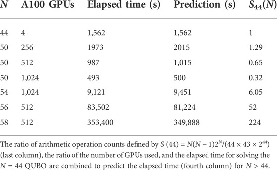
TABLE 1. Strong- and weak-scaling results for QUBO22 using NVidia A100 GPUs. The second column gives the number of GPUs used and the third column lists the elapsed time to solution.

Appendix C: Hamming distance analysis for more cases

In Figure 7 we show the normalized Hamming distance plots, averaged over 100 instances each for the 2SAT and RAN problems. It can be observed that the resulting distributions match well with the corresponding Hamming distance distributions shown in Sec. IV for the individual case. The average Hamming distance distribution peaks at 12 and 5 in case of the 2SAT and RAN problems, respectively. The average Hamming distance for the 2SAT and RAN problems are 11.07 and 8.33, respectively, while the standard deviations are 3.60 and 4.16, respectively. Since the different instances belonging to the REG class for a fixed value of N, essentially have the same problem graph, Figure 3 is a representative of all the problems of this set.

FIGURE 7

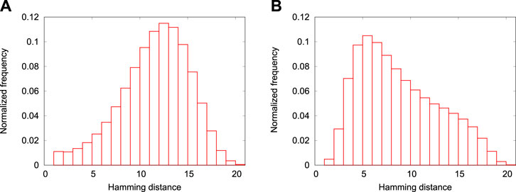
FIGURE 7. (color online) (A)Average of normalized frequencies of Hamming distances between the ground state configuration and all the first excited states, over all the 100 instances of N = 20 2SAT problems. (B) Same as (A) except that the problem instances belong to class of N = 20 RAN problems and that we only show the results for the 4,000 states which are closest to the ground state in energy. For the 2SAT problem considered, all the first excited state are degenerate.

Appendix D: Alternative fittings for the success probability

In Figures 4–6 we have used exponential functions of degree 1 in N to fit the scaling behavior of the success probability. However, we cannot, in principle, determine which function best represents the true scaling behavior of the success probability in the asymptotic limit. In this appendix, we consider other possibilities for the fitting functions. We find, upon trying exponential functions up to fourth degree polynomial in N, that exponential functions of second degree, i.e., of the kind exp (aN² + bN + c) match the scaling behavior well as shown in Figure 8.

FIGURE 8

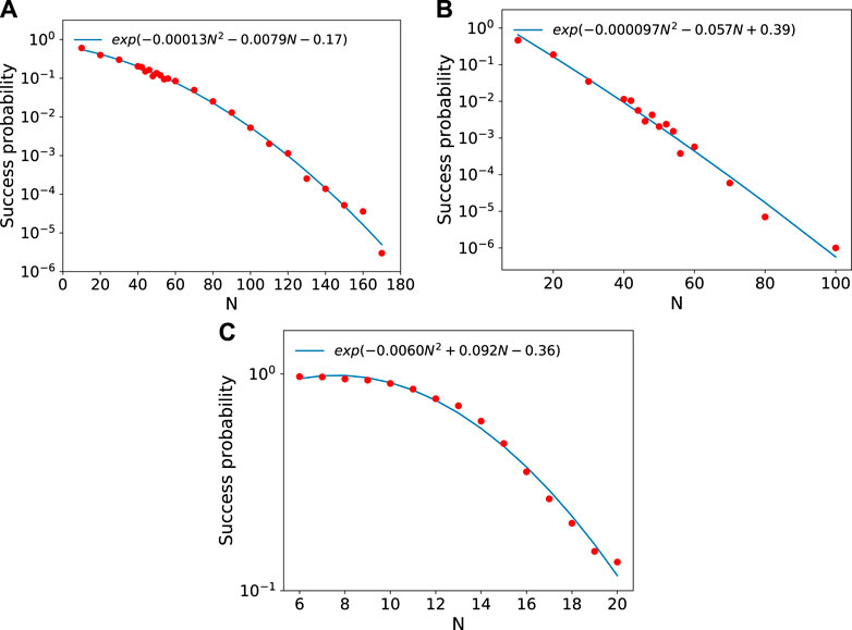
FIGURE 8. (color online) Scaling of success probability for (A) REG, (B) RAN, and (C) 2SAT classes of problems by fitting exponential functions of second degree polynomial in N.