Probabilistic Inference and Dynamic Programming: A Unified Approach to Multi-Agent Autonomous Coordination in Complex and Uncertain Environments

We present a unified approach to multi-agent autonomous coordination in complex and uncertain environments, using path planning as a problem context. We start by posing the problem on a probabilistic factor graph, showing how various path planning algorithms can be translated into specific message composition rules. This unified approach provides a very general framework that, in addition to including standard algorithms (such as sum-product, max-product, dynamic programming and mixed Reward/Entropy criteria-based algorithms), expands the design options for smoother or sharper distributions (resulting in a generalized sum/max-product algorithm, a smooth dynamic programming algorithm and a modified versions of the reward/entropy recursions). The main purpose of this contribution is to extend this framework to a multi-agent system, which by its nature defines a totally different context. Indeed, when there are interdependencies among the key elements of a hybrid team (such as goals, changing mission environment, assets and threats/obstacles/constraints), interactive optimization algorithms should provide the tools for producing intelligent courses of action that are congruent with and overcome bounded rationality and cognitive biases inherent in human decision-making. Our work, using path planning as a domain of application, seeks to make progress towards this aim by providing a scientifically rigorous algorithmic framework for proactive agent autonomy.

1 Introduction

Decision-making problems involve two essential components: the environment, which represents the problem, and the agent, which determines the solution to the problem by making decisions. The agent interacts with the environment through its decisions, receiving a reward that allows it to evaluate the efficacy of actions taken in order to improve future behavior. Therefore, the overall problem consists of a sequence of steps, in each of which the agent must choose an action from the available options. The objective of the agent will be to choose an optimal action sequence that brings the entire system to a trajectory with maximum cumulative reward (established on the basis of the reward obtained at each step). However, when the problem becomes stochastic, the main thing to pay attention to is how to evaluate the various possible rewards based on the intrinsic stochasticity of the environment. The evaluation of the reward on the basis of the probabilistic transition function leads in fact to different reward functions to be optimized. The first part of this work will show how it is possible to manage these different situations through a unified framework, highlighting its potential as a methodological element for the determination of appropriate value functions.

The present work aims to extend this framework to manage the behavior of several interdependent autonomous agents who share a common environment. We will refer to this as a multi-agent system (MAS) [1]. The type of approach to a MAS problem strongly depends on how the agents interact with each other and on the final goal they individually set out to achieve. A “fully cooperative” approach arises when the reward function is shared and the goal is to maximize the total sum of the rewards obtained by all the agents. The cooperative MAS can be further subdivided into “aware” and “unaware” depending on the knowledge that an agent has of other agents [2]. Moreover, the cooperative aware MAS can be “strongly coordinated” (the agents strictly follow the coordination protocols), “weakly coordinated” (the agents do not strictly follow the coordination protocols), and “not coordinated.” Furthermore, the agents in a cooperative aware and strongly coordinated MAS can be “centralized” (an agent is elected as the leader) or “distributed” (the agents are completely autonomous). Conversely, a “fully competitive” approach ensues when the total sum of the rewards tends to zero, and the agents implicitly compete with each other to individually earn higher cumulative rewards at the cost of other agents.

In various applications, ranging from air-traffic control to robotic warehouse management, there is the problem of centralized planning of the optimal routes. Although dynamic programming (DP) [3, 4] provides an optimal solution in the single-agent case, finding the optimal path for a multi-agent system is nevertheless complex, and often requires enormous computational costs. Obviously there are some research efforts that investigate MAS using DP [5, 6], however, they are not directly focused on the solution of a path planning problem, but rather on solving a general cooperative problem. Furthermore, it is worth noting that many research efforts are devoted to the application of reinforcement learning (RL) [7, 8] to MAS that constitutes a new research field termed multi-agent reinforcement learning (MARL) [9–11]. The main problem with reinforcement learning is the need for a large number of simulations to learn the policy for a given context, and the need to relearn when the environment changes [12]. Indeed, it is essential to understand that the agent (being autonomous but interdependent on others) must consider the actions of other agents in order to improve its own policy. In other words, from the agents’ local perspective, the environment becomes non-stationary because its best policy changes as the other agents’ policies change [9]. Moreover, as the number of agents increase, the computational complexity becomes prohibitively expensive [11].

Finally, previous works that approach the problem of path planning in a MAS context (both centralized and decentralized) do not consider regions with different rewards, ending up simply generating algorithms whose solution is the minimum path length [13]. Consideration of maps with non-uniform rewards is salient in real world scenarios: think of pedestrians that prefer sidewalks, or bikers who prefer to use bikeroutes, or ships that may use weather information to choose the best paths, etc.

The main reason for focusing on a particular problem of interest lies in the fact that knowledge of it can somehow speed up the calculations. In particular, with regards to path planning, if the goals are known to each agent a priori (as we will discuss in this work) the appropriate evaluation of the paths can be obtained using pre-computed value functions. In this case, the optimal paths can be determined without learning the policy directly, but by obtaining it on the basis of the information available from other agents. Through this work, we will show exactly how, using the knowledge of the problem and a factor graph in reduced normal form (FGrn) [14, 15], it is possible to find the optimal path in a MAS with minimal computational costs, guaranteeing an optimal solution under certain scheduling constraints. The multi-agent extension of the framework will be achieved by creating a forward flow, which will use the previously computed single-agent backward flow to enable decision making (recalling the classic probabilistic use).

Section 2 presents the Bayesian model and the corresponding factor graph in reduced normal form for the single agent case. This section shows the generality of the factor graph approach by introducing the main equations for the calculation of the value functions related to the various versions of the algorithms from probabilistic inference and operations research. Section 3 deals with the multi-agent problem, highlighting the algorithmic solution that uses the forward step coupled with the single-agent backward step, while Section 4 shows some simulation examples. Finally, in Section 5, the relevant conclusions are drawn.

2 The Single-Agent Scenario

When the outcomes generated by the actions are uncertain, because partly under the control of the agent and partly random, the problem can be defined as a Markov decision process (MDP) [16, 17]. This discrete-time mathematical tool forms the theoretical basis for the modeling of a general class of sequential decision problems in a single-agent scenario, and consequently the well-known DP, RL, and other classical decision algorithms basically aim to solve an MDP under various assumptions on the evolution of the environment and reward structure.

Mathematically, at any discrete time step t, the agent of a MDP problem is assumed to observe the state $S_t\in \mathcal{S}$ and chooses action $A_t\in \mathcal{A}$. If the sets of states and actions ($\mathcal{S}$ and $\mathcal{A}$) have a finite number of elements, the random process S_t is described as a discrete conditional probability distribution, which can be assumed to be dependent only on the previous state and action

$p\left(s_{t+1}|s_t,a_t\right)=Pr\left\{S_{t+1}=s_{t+1}|S_t=s_t,A_t=a_t\right\}$

for each admissible value of the random variables $s_{t+1},s_t\in \mathcal{S}$, and $a_t\in \mathcal{A}$. At the next time step, having moved to the state S_t+1, the agent receives a reward $r(s_t,a_t)\in \mathcal{R}\subset \mathbb{R}$ determined according to the previous state and action, thanks to which it will understand the goodness of the previous action.

A Bayesian representation of the MDP can be obtained by adding a binary random variable O_t ∈ {0, 1} (that denotes if the state-action pair at time step t is optimal or not) to the Markov chain model determined by the sequence of states and actions [18–20].

This addition (Figure 1) gives the resulting model the appearance of a hidden Markov model (HMM), in which the variable O_t corresponds to the observation. In this way, at each time step, the model emits an “optimality” measure in the form of an indicator function, which leads to the concept of “reward” necessary to solve the problem of learning a policy π(a_t|s_t) (highlighted in red in Figure 1) that maximizes the expected cumulative reward. Assuming a finite horizon T, ¹ the joint probability distribution of the random variables in Figure 1 can therefore be factored as follows

$p\left(s_1,a_1,o_1,\dots ,s_T,a_T,o_T\right)=p\left(s_1\right)p\left(a_T\right)p\left(o_T|s_T,a_T\right)\prod _{t=1}^{T-1}p\left(s_{t+1}|s_t,a_t\right)p\left(a_t\right)p\left(o_t|s_t,a_t\right)$

where p(a_t) is the prior on the actions at time step t. In other words, the introduction of the binary random variable O_t represents a “trick” used by the stochastic model to be able to condition the behavior of the agent at time step t, so that it is “optimal” from the point of view of the rewards that the agent can get. Specifically, defining with c (s_t, a_t) the general distribution of the random variable O_t, we obtain that when O_t = 0, there is no optimality and

$p\left(O_t=0|s_t,a_t\right)\triangleq c\left(s_t,a_t\right)\propto \mathcal{U}\left(s_t,a_t\right).$

where $\mathcal{U}(s_t,a_t)$ is the uniform distribution over states and actions, implying the agent has no preference to any particular state and action of the MDP. Vice-versa optimality with O_t = 1 corresponds to

$p\left(O_t=1|s_t,a_t\right)\triangleq c\left(s_t,a_t\right)\propto \exp \left(r\left(s_t,a_t\right)\right)$

where r (s_t, a_t) is the reward function and the exponential derives from opportunistic reasons that will be clarified shortly. Since what really matters is the optimal solution obtained by conditioning on O_t = 1 for every t = 1, … , T, we can also omit the sequence{O_t} from the factorization, and rewrite the joint distribution of state-action sequence over [0, T] conditioned on optimality as

$\begin{array}{ll}\hfill p\left(s_1,a_1,\dots ,s_T,a_T|O_{1:T}=\mathbf{1}\right)& =p^{\ast }\left(s_1,a_1,\dots ,s_T,a_T\right)\hfill \\ \hfill & \times \propto p\left(s_1\right)p\left(a_T\right)c\left(s_T,a_T\right)\prod _{t=1}^{T-1}p\left(s_{t+1}|s_t,a_t\right)p\left(a_t\right)c\left(s_t,a_t\right)\hfill \end{array}$

It can thus be noted that

$p^{\ast }\left(s_1,a_1,\dots ,s_T,a_T\right)\propto \left[p\left(s_1\right)p\left(a_T\right)\prod _{t=1}^{T-1}p\left(s_{t+1}|s_t,a_t\right)p\left(a_t\right)\right]\times \exp \left(\sum _{t=1}^{T}r\left(s_t,a_t\right)\right)$

and therefore, through the previous definition of the function c(s_t, a_t) as the exponential of the reward function, the probability of observing a given trajectory also becomes effectively dependent on the total reward that can be accumulated along it.

FIGURE 1

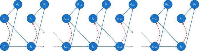
FIGURE 1. Bayesian graph of the generative model of an MDP, in which the variable O_t represents the optimum for that time step.

2.1 The Factor Graph

The probabilistic formulation of the various control/estimation algorithms based on MDP can be conveniently translated into a factor graph (FG) [21–23], in which each variable is associated with an arc and the various factors represent its interconnection blocks. In particular, we will see how it is extremely useful to adopt the “reduced normal form” (introduced previously) which allows, through the definition of “shaded” blocks, to map a single variable in a common space; simplifying the message propagation rules through a structure whose functional blocks are all SISO (single-input/single-output). The Bayesian model of interest in Figure 1 can in fact be easily translated into the FGrn of Figure 2, where the a priori distributions p(a_t) and c(s_t, a_t) are mapped to the source nodes, and the probabilities of transition p(s_t+1|s_t, a_t) are implemented in the $\mathcal{M}$ SISO blocks. Each arc is associated with a “forward” f and a “backward” b message, proportional to the probability distributions and whose composition rules allow an easy propagation of the probability; while, as usual, the diverter (in red) represents the equality constraint between the variables that belong to it. Furthermore, using this structure, one has the advantage of easily introducing constraints and a priori knowledge into the corresponding messages that propagate through them. ² In general, all available evidence can in fact be collectively identified through the symbol K_1:T, so that we can describe the model in the form p*(s₁, a₁, … , s_T, a_T|K_1:T) during the process of inference. For the defined graph, we therefore aim to compute mainly the functions

$\begin{array}{ll}\hfill p^{\ast }\left(s_t|K_{1:T}\right)& \propto \sum _{\begin{array}{c}{s}_j,j=1:T,j\ne t\\ a_k,k=1:T\end{array}}{p}^{\ast }\left(s_1,a_1,\dots ,s_T,a_T|K_{1:T}\right)\hfill \\ \hfill p^{\ast }\left(s_t,a_t|K_{1:T}\right)& \propto \sum _{\begin{array}{c}{s}_j,a_j,j=1:T,j\ne t\end{array}}{p}^{\ast }\left(s_1,a_1,\dots ,s_T,a_T|K_{1:T}\right)\hfill \end{array}$

which, for example, can be derived from message propagation through the use of the classic sum-product rule [22, 24]. Note that these are the only functions needed for our purposes because the optimal policy at time t can be obtained by

${\pi }^{\ast }\left(a_t|s_t\right)\triangleq p^{\ast }\left(a_t|s_t,K_{t:T}\right)=\frac{p^{\ast }\left(s_t,a_t|K_{t:T}\right)}{p^{\ast }\left(s_t|K_{t:T}\right)},t=1:T$

By rigorously applying Bayes’ theorem and marginalization, the various messages propagate within the network and contribute to the determination of the posteriors through the simple multiplication of the relative forward and backward messages [14, 25]. In particular, from Figure 2, it can be seen that the calculation of the distribution for the policy at time t can generally be rewritten as

${\pi }^{\ast }\left(a_t|s_t\right)\propto \frac{f_{{\left(S_t,A_t\right)}^{\left(i\right)}}\left(s_t,a_t\right)b_{{\left(S_t,A_t\right)}^{\left(i\right)}}\left(s_t,a_t\right)}{f_{S_t}\left(s_t\right)b_{S_t}\left(s_t\right)}=\frac{f_{S_t}\left(s_t\right)\mathcal{U}\left(a_t\right)b_{{\left(S_t,A_t\right)}^{\left(i\right)}}\left(s_t,a_t\right)}{f_{S_t}\left(s_t\right)b_{S_t}\left(s_t\right)}=\frac{b_{{\left(S_t,A_t\right)}^{\left(i\right)}}\left(s_t,a_t\right)}{b_{S_t}\left(s_t\right)}$

and, therefore, the policy depends solely on the backward flow, ³ since (by conditioning on s_t) all the information coming from the forward direction is irrelevant to calculate it. ⁴

FIGURE 2

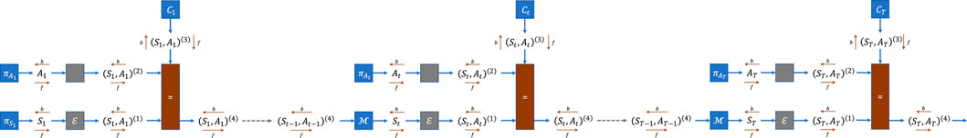
FIGURE 2. Factor Graph in reduced normal form of an MDP, in which the reward is introduced through the variable C_t.

Particularly interesting is the passage from the probabilistic space to the logarithmic space, which, within the FGrn, can be obtained through the simple definition of the functions

$\begin{array}{ll}\hfill V_{S_t}\left(s_t\right)& \triangleq \ln b_{S_t}\left(s_t\right)\hfill \\ \hfill Q_{{\left(S_t,A_t\right)}^{\left(i\right)}}\left(s_t,a_t\right)& \triangleq \ln b_{{\left(S_t,A_t\right)}^{\left(i\right)}}\left(s_t,a_t\right),i=1,\dots ,4\hfill \end{array}$

whose name is deliberately assigned in this way to bring to mind the classic DP-like approaches. ⁵ Looking at Figure 2, the backward propagation flow can then be rewritten considering the passage of messages through the generic transition operators represented by the blocks $\mathcal{M}[\cdot ]$ and $\mathcal{E}[\cdot ]$ shown as

$\begin{array}{ll}\hfill V_{S_t}\left(s_t\right)& \propto \mathcal{E}\left[Q_{{\left(S_t,A_t\right)}^{\left(1\right)}}\left(s_t,a_t\right)\right]\hfill \\ \hfill Q_{{\left(S_t,A_t\right)}^{\left(1\right)}}\left(s_t,a_t\right)& \propto \ln p\left(a_t\right)+r\left(s_t,a_t\right)+\mathcal{M}\left[V_{S_{t+1}}\left(s_{t+1}\right)\right]\hfill \\ \hfill & =R\left(s_t,a_t\right)+Q_{{\left(S_t,A_t\right)}^{\left(4\right)}}\left(s_t,a_t\right)\hfill \end{array}$

where R(s_t, a_t) = ln p(a_t) + r(s_t, a_t). Although, in the classic sum-product algorithm, these blocks correspond to a marginalization process, it is still possible to demonstrate that the simple reassignment of different procedures to them allows one to obtain different types of algorithms within the same model [25]. Supplementary Appendix S1 presents various algorithms that can be used simply by modifying the function within the previous blocks, and which, therefore, show the generality of this framework, while Table 1 summarizes the related equations by setting $Q(s_t,a_t)=Q_{{(S_t,A_t)}^{(1)}}(s_t,a_t)$ and $V(s_t)=V_{S_t}(s_t)$. It should also be noted that, for all the algorithms presented in the Supplementary Appendix, the definition of the policy can always be described according to the V and Q functions, by setting

${\pi }^{\ast }\left(a_t|s_t\right)\propto \exp \left(Q_{{\left(S_t,A_t\right)}^{\left(1\right)}}\left(s_t,a_t\right)-V_{S_t}\left(s_t\right)\right)$

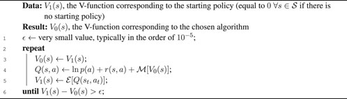
We emphasize the ease with which these algorithms can be evaluated via FGrn, as they can be defined through a simple modification of the base blocks. The pseudocode presented in Algorithm 1 highlights this simplicity, using the generic transition blocks just defined (and illustrated in Figure 2) whose function depends on the chosen algorithm.

TABLE 1

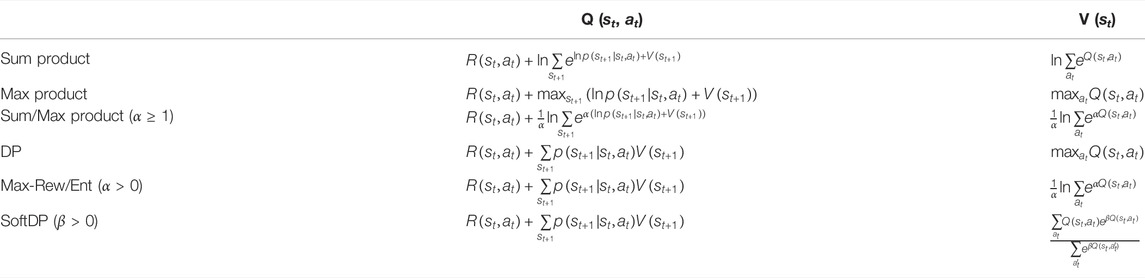
TABLE 1. Summarized backup rules in log space.

Algorithm 1. Algorithm for the generic V-function

3 The Multi-Agent Scenario

As stated above, when we have a problem with more than one agent, the computation of the value function collides with the complexity of a changing environment. More specifically, if all agents move around seeking their goals, the availability of states changes continuously and in principle the value functions have to be recalculated for each agent at every time step. Therefore, the problem is no longer manageable as before, and in general it must be completely reformulated to be tractable in many problem contexts.

The theoretical framework to describe a MAS is the Markov game (MG) [26, 27], that generalizes the MDP in the presence of multiple agents. Differently from the single agent MDP, in the multiple agent context, the transition probability function and the rewards depend on the joint action ${\mathit{A}}_t\in \mathcal{A}$, where $\mathcal{A}={\mathcal{A}}_1\times {\mathcal{A}}_2\dots \times {\mathcal{A}}_n$ with n agents. At each time step t, the ith agent selects an action from its own action space ${\mathcal{A}}_i$ (simultaneously with other agents) and the system evolves following the transition probability function $P:\mathcal{S}\times \mathcal{A}\to [\mathrm{0,1}]$ and generates the reward $R_i:\mathcal{S}\times \mathcal{A}\times \mathcal{S}\to \mathcal{R}\subset \mathbb{R}$. Consequently, the value function will not only depend on the policy of the single ith agent, but also on all other agents [10, 11]. In other words, considering the general case of an infinite horizon discounted version of the stochastic path planning problem, with a reward function that depends on current state-action pair as well as the next state, the value function for the ith agent will be

$V_{{\pi }_i,{\mathit{\pi }}_{-i}}^{\left(i\right)}\left(s\right)={\mathbb{E}}_{s_{t+1}\sim P,a_t\sim \mathit{\pi }}\left[\sum _{t=0}^{\infty }{\gamma }^t{R}_i\left(s_t,a_t,s_{t+1}\right)|s=s_0\right](1)$

where a_t ∈ A_t, π = {π₁, … , π_n} is the joint policy, π_−i = {π₁, … , π_i−1, π_i+1, π_n} is the policy of all other agents except the ith and γ ∈ [0, 1] is a discount rate.

The above problem, when the state space and the number of agents grow, becomes very quickly intractable. Therefore, we have to resort to simplifications, such as avoiding the need to consider the global joint spaces, and adopting simplifying distributed strategies that are sufficiently general to be applicable to practical scenarios. We focus here on a path planning problem for multiple agents that act sequentially, are non-competitive, share centralized information and are organized in a hierarchical sequence. Within these constraints, in fact, we will see how it is possible to use the versatility of the FGrn formulation by leveraging just one pre-calculated value function for each goal.

3.1 The Environment

Consider a scenario with n agents moving around a map with a given reward function r(s_t) that depends only on the state. The rewards may represent preferred areas, such as sidewalks for pedestrians, streets for cars, bike routes for bicycles, or related to the traffic/weather conditions for ships and aircraft, etc. Therefore, at each time step, the overall action undertaken by the system is comprised of the n components

$a_t=\left(a_t^{\left(1\right)},\dots ,a_t^{\left(n\right)}\right)$

where $a_t^{(i)}$ represents the action performed by the ith agent at time step t. The map is a discrete rectangular grid of dimensions N × M that defines the state space $\mathcal{S}$, in the sense that each free cell of the grid determines a state reachable by the agents. We assume that both the map and the reward function linked to the various states are the same for each agent, but that each agent aims to reach its own goal (some goals may coincide).

The objectives of each agent may represent points of interest in a real map, ⁶ and the existence of different rewards in particular areas of the map may correspond to preference for movement through these areas. The ultimate goal is to ensure that each agent reaches its target by accumulating the maximum possible reward, despite the presence of other agents. We assume that every action towards an obstacle, the edge of the map or another agent, constrains the agent to remain in the same state (reflection), setting a reward that is never positive (in our formulation the rewards are all negative, except on the goal, where it is null). Furthermore, it is assumed that in the time step following the achievement of the objective, the agent no longer occupies any position on the map (it disappears). This ensures that arriving at the destination does not block the subsequent passage of other agents through that state, which could otherwise make the problem unsolvable.

3.2 The Forward Propagation

This MAS problem is ideally suited for approximate solution using FGrn, performing just some small changes similar to those introduced previously for the various objective functions. In particular, we will show how each agent will be able to perform its own inference on its particular FGrn (taking into account the target and the presence of other agents) simply by establishing an appropriate forward message propagation process. To do this, first, it is assumed that each agent follows a strict scheduling protocol, established in advance, to choose the action to perform. To fix the ideas, the agents are numbered in order of priority from 1 to n. Therefore, the ith agent will be allowed to perform its action at time t only after all the previous agents (from 1 to i − 1) have performed their tth step. In this way, similarly to what [12] proposed, the time step t is decomposed into n different sub-steps, relating to the n agents present on the scene. Since each agent’s information is assumed to be shared with every other agent, and each agent is assumed to have access to this centralized information, the use of a scheduling protocol provides the next agent with the future policy of the agents who will move first, allowing it to organize its steps in relation to them. The idea is akin to Gauss-Seidel approach to solving linear equations and to Gibbs sampling.

Integrating this information into the FGrn is extremely simple. By looking at Figure 3, it is sufficient to make block C_t also dependent on the optimal trajectory at time t that the previous agents have calculated (calculated but not yet performed!) for themselves. In other words, at each time step, block C_t provides to each agent i a null value (in probabilistic space) for those states that are supposed to be occupied by the other agents. In this way, the ith agent will be constrained to reach its goal avoiding such states. Focusing on a specific agent i (dropping the index for notational simplicity), a priori knowledge on the initial state $S_1={\widehat{s}}_1$ can be injected through a delta function ⁷ in the relative probabilistic forward message

$f_{S_1}\left(s_1\right)=\delta \left(s_1-{\widehat{s}}_1\right)$

and assuming that $\mathcal{M}$ blocks in FGrn perform the function

$f_{S_{t+1}}\left(s_{t+1}\right)=\underset{s_t,a_t}{\max }p\left(s_{t+1}|s_t,a_t\right)f_{{\left(S_t,A_t\right)}^{\left(4\right)}}\left(s_t,a_t\right)$

with

$f_{{\left(S_t,A_t\right)}^{\left(4\right)}}\left(s_t,a_t\right)=f_{{\left(S_t,A_t\right)}^{\left(1\right)}}\left(s_t,a_t\right)f_{{\left(S_t,A_t\right)}^{\left(2\right)}}\left(s_t,a_t\right)c\left(s_t,a_t\right)$

the FGrn autonomously modifies its behavior by carrying out a process of pure diffusion which determines the best possible trajectory to reach a given state in a finite number of steps.

FIGURE 3

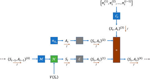
FIGURE 3. Modified version of FGrn for the Multi-Agent forward step. Each agent will have its own factorial graph, in which information from previous agents (within the scheduling process) modifies the C_t variable. The algorithm block $\mathcal{H}$, which analyzes the value function to block the propagation of superfluous projections is shown in green.

Note that this propagation process leads to optimality only if we are interested in evaluating the minimum-time path [28]. ⁸ Although the reward is accumulated via c (s_t, a_t), the forward process totally ignores it, not being able to consider other non-minimal paths that could accumulate larger rewards. In fact, exhaustively enumerating all the alternatives may become unmanageable, unless we are driven by another process. In other words, this propagation process alone does not guarantee that the first accumulated value with which a goal state is reached, is the best possible. Further exploration, without being aware of the time required to obtain the path of maximum reward, may force us to run the algorithm for a very large number of steps (with increasing computational costs). However, as mentioned above, the reference scenario involves goals that are independent and are known a priori. This means that (through any of the algorithms discussed in Supplementary Appendix S1) it is possible to calculate the value function in advance for each goal. Note that this offline calculation is independent of the location/presence of the agents in the MAS scenario and therefore could not be used directly to determine the overall action a_t of the system. The following lemma is useful to claim optimality.

LEMMA 1. The value function computed by excluding the agents from the scene represents an upper-bound (in terms of cumulative reward) for a given state.

Proof. : The demonstration is trivial as other agents (being moldable as dynamic obstacles) can only reduce the value obtained from the value function for the agent, by hindering a valid passage through their presence and forcing the agent to traverse a sub-optimal path.Knowing the value function corresponding to the objective of a particular agent, it is therefore possible to limit the $f_{S_{t+1}}(s_{t+1})$ only to the values that actually have the possibility of reaching the goal with an accumulated reward larger than the current value. In other words, at each time step t, after the diffusion arrives on the goal, it is possible to add the value function to the $\ln f_{S_{t+1}}(s_{t+1})$ to compare the active states with the value currently obtained on the goal, eliminating all those paths that could not in any way reach the objective with a higher cumulative reward (since, as mentioned, this represents an upper-bound for every possible state). The only projections left will represent possible steps towards better solutions and will continue to propagate to determine if their dynamics can actually enable the discovery of a better path. To highlight this step, in Figure 3, this addition is shown using a $\mathcal{H}$ block (placed separately from the $\mathcal{M}$ block only to facilitate understanding), which takes the pre-computed V-function as input and performs the three algorithmic operations just described (addition, comparison and elimination). The pseudocode of the forward process for the single ith agent is shown in Algorithm 2.

Algorithm 2. Algorithm for the forward propagation in a MAS context using the V-functions

A better understanding of the whole forward propagation process is perhaps achievable by considering the trellis of Figure 4, which shows the forward propagation flow for a “blue” agent given the trajectory decided by the “yellow” agent. The trellis shows the various steps on the abscissa (from t₁ to t₁₇) and the accessible states of the map on the ordinate (from s⁽¹⁾ to s⁽³⁶⁾), highlighting the states related to the two different objectives through rectangles of the respective colors. The blue agent propagates its projections to various time steps taking into account the possible actions, avoiding the states already occupied and considering only the paths with the maximum cumulative reward (the other paths not chosen are graphically represented in light gray).From the moment a path to the goal is found (t₁₂), the $\mathcal{H}$ block of Figure 3 performs its tasks by blocking the propagation of projections that have no chance of improving the value of the final cumulative reward (all gray circles reached by an arrow at t₁₂ and in subsequent time steps). ⁹ This also means that if another path is able to reach the goal again, then it will certainly be better than the previous one. In other words, when the control block clears all projections on the map, then the last path that was able to get to the goal is chosen as the preferred trajectory for the agent. In the example of Figure 4, the blue agent reaches the goal again at t₁₃ and the cumulative reward is higher than the one obtained at t₁₂, but the projections can continue through the state s⁽³⁾ that allows us to reach the goal at time step t₁₇. Since, at that time step, all the other projections have been blocked, the path (in black) from s⁽²⁴⁾ at t₁ to s⁽⁹⁾ at t₁₇ is optimal.

FIGURE 4

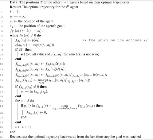
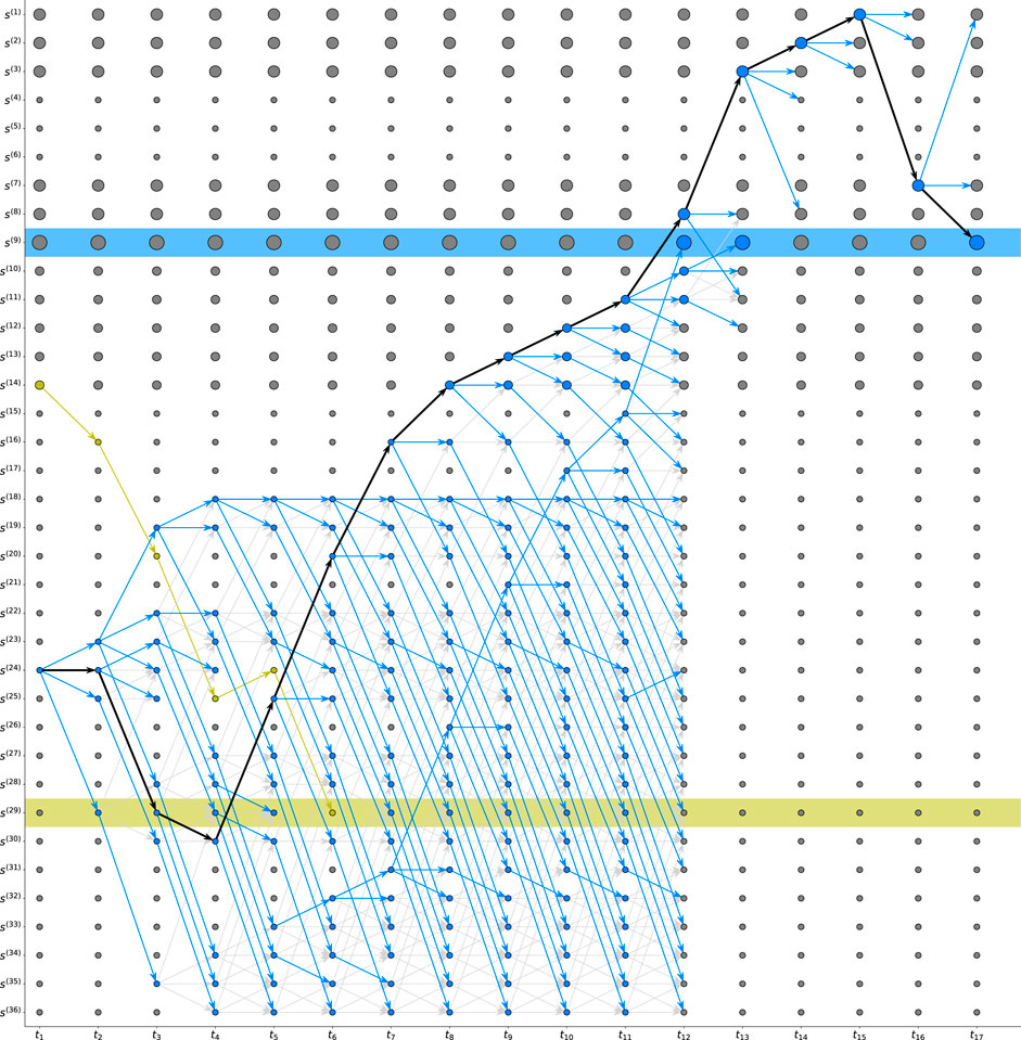
FIGURE 4. Trellis related to the analysis of the optimal path for the blue agent based on the preliminary presence of the yellow agent. The highest reward map states are represented by larger circles. The blue arrows represent the forward propagated projections, while the light gray ones denote the other discarded possibilities. The optimal path determined by forward propagation within the FGrn is represented in black.

4 Simulations

If the environment is assumed to be fully deterministic, each agent will have to calculate its optimal trajectory only once and, when all agents have performed the calculation, the movements can be performed simultaneously. In such circumstances, a good scheduling protocol can be obtained by sorting agents according to

$\underset{s\in N\left(s_1\right)\subseteq \mathcal{S}\backslash \widehat{\mathcal{S}}}{\max }V\left(s\right)$

where N (s₁) is the neighborhood of s₁ given the feasible actions of the agent, and $\widehat{S}$ is the set of states relative to the initial positions of all agents. In this way, the agents closest to their respective goals will move independently from the others, arriving first and being irrelevant for the subsequent steps necessary for the other agents. In the various simulations conducted in deterministic environments, this choice has always proved successful, reaching the maximum total reward for all agents compared to any other possible scheduling sequence. However, the forward procedure guarantees the optimal solution for the particular scheduling sequence chosen. In fact, at each time step, the algorithm considers the maximum for each possible state-action pair, blocking all those paths that (even at their maximum) would never be able to reach the goal. In practice, the upper bound constituted by the value function allows us to avoid considering every possible path, but guarantees us that all the excluded paths are certainly worse. All the paths that the algorithm considers are therefore certainly the best possible, and for this reason the optimal path for the agent in that given scheduling sequence is guaranteed. The overall optimality, in relation to the sum of all the cumulative rewards obtained by each agent, is, however, strongly linked to the chosen scheduling procedure, that can therefore lead to non-optimal solutions, if not appropriately chosen. ¹⁰ A simple simulation with two agents is shown in Figure 5, where it is assumed that the action space is composed of only four elements $\mathcal{A}=$ {up, down, left, right} and that the reward is always equal to −10 except on green states, where it is equal to −1. It can be seen that the blue agent chooses the longest path which, however, represents the one with the higher cumulative reward, due to the presence of a higher reward area. Despite this, from the beginning, the yellow agent blocks the path of the blue one, who is therefore forced to move around until it becomes free (t₅). After this time step, the two agents can reach their respective goals without any interaction. ¹¹ A further example, more complex than the previous one, is shown in Figure 6. In this case, the action space is composed of eight elements $\mathcal{A}=$ {top-left, up, top-right, left, right, down-left, down, down-right} with n = 4 agents present on the map. It is worth noting how the red agent at t₇, t₈, t₉, t₁₀ wanders around in the region with a high reward in order to wait for the purple agent to go through the tunnel and accumulate a higher reward. In the deterministic case, the computational cost of the online procedure is extremely low, as it can be evaluated in $\mathcal{O}(n\log NM)$ in the worst case.

FIGURE 5

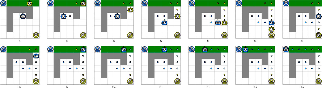
FIGURE 5. Representation of the movement of two agents on a small map in a deterministic environment. Both agents have only four possible actions {up, down, left, right}. The value function is calculated through the DP and both agents have their own goals.

FIGURE 6

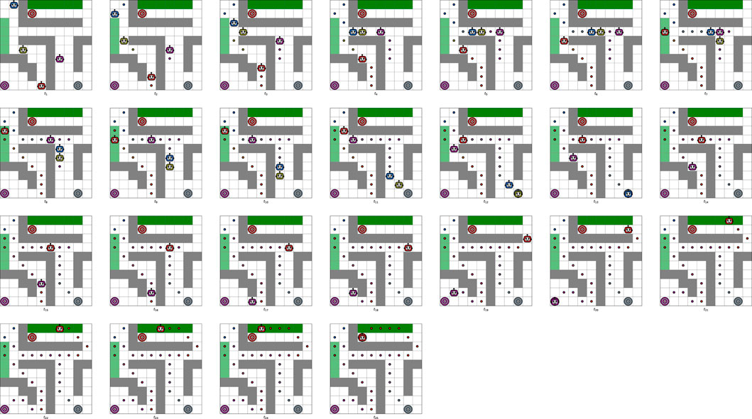
FIGURE 6. Representation of the movement of four agents in a deterministic environment with eight possible actions {top-left, up, top-right, left, right, down-left, down, down-right}. The value function is calculated through the DP and the blue and yellow agents share the same goal while purple and red agents have their own goals.

General behavior does not change in the case in which a non-deterministic transition dynamics are assumed, i.e., assuming the agents to be in an environment in which every action does not necessarily lead to the state towards which the action points; providing a certain (lesser) probability of ending up in a different state among those admissible (as if some other action had actually been performed). ¹² What changes, however, is the total computational cost. Each time the agent takes a step, in fact, if the step does not fall within the optimal trajectory calculated previously, then it will be forced to recalculate its trajectory again to pass it to other subsequent agents.

It must be considered, however, that each calculation has a low computational cost anyway (definitely much lower than the total recalculation of the value function) and that, at each step, the agents get closer and closer to their goals (making the calculation faster, because it is always less likely to find better alternative routes). These considerations are obviously strictly linked to the uncertainty present in the system. To clarify these observations, in Figure 7 the same diagram of the deterministic environment of Figure 6 is presented, with the same four agents positioned within the same map. This time, however, it is assumed to use an action tensor that results in a random error of 5% equally distributed on adjacent actions (i.e., close to the action contemplated). A graphical representation of the action tensor, considering the agent positioned at the center of each grid cell, is shown in Figure 8. A comparison with the deterministic case of Figure 6 allows us to understand the behaviors stemming exclusively from the stochasticity of the environment. For example, it can be observed how the blue agent is pushed in the opposite direction to the action taken (from time step 7–11), but nevertheless correctly recalculates its trajectory to allow others to take their paths based on the mistakes made. Note that, in the stochastic case, the optimality on the single execution cannot be guaranteed, precisely because of the intrinsic stochasticity of the environment. However, this argument is general and is valid for any algorithm in a stochastic environment. Furthermore, it must be said that if it were possible to regenerate an optimal scheduling sequence at each variation with respect to the previously calculated trajectory, it could be stated that on multiple executions (since the algorithm maximizes the likelihood and since each sub-trajectory would be optimal), the behavior tends asymptotically to the optimum.

FIGURE 7

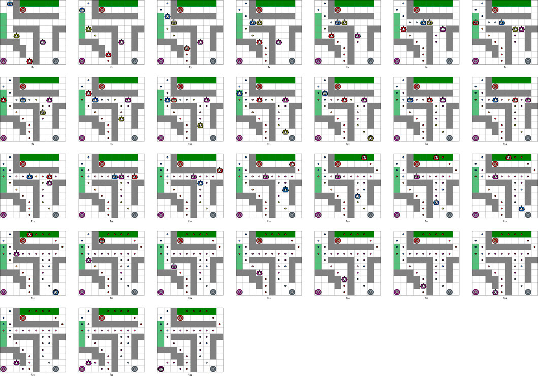
FIGURE 7. Representation of the movement of four agents in stochastic environment with a 5% chance of error on neighboring actions and eight possible actions {top-left, up, top-right, left, right, down-left, down, down-right}.

FIGURE 8

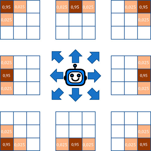
FIGURE 8. Action probability tensor with an error probability of 5% on neighboring actions.

5 Conclusion

We have shown how it is possible to unify probabilistic inference and dynamic programming within an FGrn through specific message composition rules. The proposed framework allows various classical algorithms (sum-product, max-product, dynamic programming and based on mixed reward/entropy criteria), also by expanding the algorithmic design options (through generalized versions), only by modifying the functions within the individual blocks.

Using a path planning problem context, we have also shown how this framework proves to be decidedly flexible, and how it is possible to use it even in the multi-agent case. Moreover, the forward procedure turns out to be very fast in calculating the optimal trajectory subject to an agent scheduling protocol. The use of the value function as upper bound allows, in fact, to limit the propagation of the projections at the various time steps, accelerating and guaranteeing the achievement of the optimal solution in deterministic cases (again subject to a specified agent scheduling protocol). The proposed simulations have shown how the solution is effective even in a stochastic environment, where the optimal solution is not reachable on a single example due to the intrinsic variability of the environment.

We believe that the work presented here provides a scientifically rigorous algorithmic framework for proactive agent autonomy. The factor graph-based message propagation approach to MAS will enable us to investigate the interdependencies among the key elements of a hybrid team, such as goals, changing mission environment, assets and threats/obstacles/constraints. We believe that the interactive optimization algorithms based on this approach should provide the tools for producing intelligent courses of action that are congruent with and overcome bounded rationality and cognitive biases inherent in human decision-making.

Data Availability Statement

The original contributions presented in the study are included in the article/Supplementary Material, further inquiries can be directed to the corresponding author.

Author Contributions

GD, conceptualization, methodology, writing-original draft, writing-review and editing, visualization, and software. AB, conceptualization, methodology, writing-original draft, writing-review and editing, and visualization. GF and FV, visualization, software, writing-review and editing. KP and FP, conceptualization, methodology, visualization, supervision, writing-review and editing, and funding acquisition.

Funding

This work was supported in part by POR CAMPANIA FESR 2014/2020, ITS for Logistics, awarded to CNIT (Consorzio Nazionale Interuniversitario per le Telecomunicazioni). Research of Pattipati was supported in part by the US Office of Naval Research and US Naval Research Laboratory under Grants #N00014-18-1-1238, #N00014-21-1-2187, #N00173-16-1-G905 and #HPCM034125HQU.

Conflict of Interest

The authors declare that the research was conducted in the absence of any commercial or financial relationships that could be construed as a potential conflict of interest.

Publisher’s Note

All claims expressed in this article are solely those of the authors and do not necessarily represent those of their affiliated organizations, or those of the publisher, the editors and the reviewers. Any product that may be evaluated in this article, or claim that may be made by its manufacturer, is not guaranteed or endorsed by the publisher.

Supplementary Material

The Supplementary Material for this article can be found online at: https://www.frontiersin.org/articles/10.3389/fphy.2022.944157/full#supplementary-material

Footnotes

¹Note that we consider the time horizon T as the last time step in which an action must be performed. The process will stop at instant T + 1, where there is no action or reward.

²Think, for example, of a priori knowledge about the initial state or even more about the initial action to be performed.

³The index i is used in general terms, since for each i = 1, … , 4, the value of the product between forward and backward (referring to the different versions of the joint random variable in Figure 2) is always identical.

⁴This is consistent with the principle of optimality: given the current state, the remaining decisions must constitute an optimal policy. Consequently, it is not surprising that the backward messages have all the information to compute the optimal policy.

⁵From the definition provided, it is understood that in this case the functions will always assume negative values. However, this is not a limitation because one can always add a constant to make rewards nonnegative.

⁶For example, the targets could be gas stations or ports (in a maritime scenario), whose presence on the map is known regardless of the agents.

⁷We refer to the Kronecker Delta δ(x), which is equal to 1 if x = 0 and is zero otherwise.

⁸The very concept of “time” in this case can be slightly misleading. The reward function linked to individual states can in fact represent the time needed to travel in those states (for example due to traffic, or adverse weather conditions). In this case, the number of steps performed by the algorithm does not actually represent the “time” to reach a certain state. We emphasize that in the presence of a reward/cost function, the objective is not to reach a given state in the fewest possible steps, but to obtain the highest/lowest achievable reward/cost.

⁹Note that the $\mathcal{H}$ block actually exists at each step t of the process described, but since the deletion of projections occurs by comparing the sum with the value currently present on the target (and since, at the beginning, this value is considered infinitely negative), the block will practically never delete any projections until the target is achieved for the first time.

¹⁰The search for an optimal scheduling choice is under consideration and will be published elsewhere.

¹¹It should be noted that a different scheduling choice would lead to the yellow agent being blocked by the blue agent, obtaining an overall reward for both agents lower than that obtained.

¹²To make the concept realistic, one can imagine an environment with strong winds or with large waves. In general, this reference scenario aims to perform the control even in the presence of elements that prevent an exact knowledge of the future state following the chosen action.

References

1. Weiss G. Multiagent Systems. 2nd ed. Cambridge: MIT Press (2016).

Google Scholar

2. Farinelli A, Iocchi L, Nardi D. Multirobot Systems: a Classification Focused on Coordination. IEEE Trans Syst Man Cybern B Cybern (2004) 34:2015–28. doi:10.1109/tsmcb.2004.832155

PubMed Abstract | CrossRef Full Text | Google Scholar

3. Bellman RE. Dynamic Programming. New York: Dover (2003).

Google Scholar

4. Bertsekas DP. Dynamic Programming And Optimal Control (Athena) (2017). Cambridge: Athena.

Google Scholar

5. Szer D, Charpillet F. Point-Based Dynamic Programming for Dec-Pomdps. Association for the Advancement of Artificial Intelligence (2006) 6:1233–8.

Google Scholar

6. Bertsekas D. Multiagent Value Iteration Algorithms in Dynamic Programming and Reinforcement Learning. Results in Control and Optimization (2020) 1:1–10. doi:10.1016/j.rico.2020.100003

CrossRef Full Text | Google Scholar

7. Sutton RS, Barto AG. Reinforcement Learning: An Introduction. Cambridge: The MIT Press (2018).

Google Scholar

8. Bertsekas DP. Reinforcement Learning And Optimal Control (2019). Cambridge: Athena

Google Scholar

9. Busoniu L, Babuska R, De Schutter B. A Comprehensive Survey of Multiagent Reinforcement Learning. IEEE Trans Syst Man Cybern C (2008) 38:156–72. doi:10.1109/tsmcc.2007.913919

CrossRef Full Text | Google Scholar

10. Nowé A, Vrancx P, De Hauwere Y-M. Game Theory and Multi-Agent Reinforcement Learning. In: M Wiering, and M van Otterlo, editors. Reinforcement Learning: State-Of-The-Art. Berlin, Heidelberg: Springer (2012). p. 441–70. doi:10.1007/978-3-642-27645-3_14

CrossRef Full Text | Google Scholar

11. Yang Y, Wang J. An Overview of Multi-Agent Reinforcement Learning from Game Theoretical Perspective. arXiv (2020). Available at: https://arxiv.org/abs/2011.00583.

Google Scholar

12. Bertsekas D. Multiagent Reinforcement Learning: Rollout and Policy Iteration. Ieee/caa J Autom Sinica (2021) 8:249–72. doi:10.1109/jas.2021.1003814

CrossRef Full Text | Google Scholar

13. Lejeune E, Sarkar S. Survey of the Multi-Agent Pathfinding Solutions (2021). doi:10.13140/RG.2.2.14030.28486

CrossRef Full Text | Google Scholar

14. Palmieri FAN. A Comparison of Algorithms for Learning Hidden Variables in Bayesian Factor Graphs in Reduced normal Form. IEEE Trans Neural Netw Learn Syst. (2016) 27:2242–55. doi:10.1109/tnnls.2015.2477379

PubMed Abstract | CrossRef Full Text | Google Scholar

15. Di Gennaro G, Buonanno A, Palmieri FAN. Optimized Realization of Bayesian Networks in Reduced normal Form Using Latent Variable Model. Soft Comput (2021) 10:1–12. doi:10.1007/s00500-021-05642-3

CrossRef Full Text | Google Scholar

16. Bellman R. A Markovian Decision Process. Indiana Univ Math J (1957) 6:679–84. doi:10.1512/iumj.1957.6.56038

CrossRef Full Text | Google Scholar

17. Puterman ML. Markov Decision Processes: Discrete Stochastic Dynamic Programming. New York: Wiley (2005).

Google Scholar

18. Kappen HJ, Gómez V, Opper M. Optimal Control as a Graphical Model Inference Problem. Mach Learn (2012) 87:159–82. doi:10.1007/s10994-012-5278-7

CrossRef Full Text | Google Scholar

19. Levine S. Reinforcement Learning and Control as Probabilistic Inference: Tutorial and Review. arXiv (2018). Available at: https://arxiv.org/abs/1805.00909

Google Scholar

20. O’Donoghue B, Osband I, Ionescu C. Making Sense of Reinforcement Learning and Probabilistic Inference. In: 8th International Conference on Learning Representations (ICLR) (OpenReview.net) (2020).

Google Scholar

21. Forney GD. Codes on Graphs: normal Realizations. IEEE Trans Inform Theor (2001) 47:520–48. doi:10.1109/18.910573

CrossRef Full Text | Google Scholar

22. Koller D, Friedman N. Probabilistic Graphical Models: Principles and Techniques. Cambridge: The MIT Press (2009).

Google Scholar

23. Loeliger H. An Introduction to Factor Graphs. IEEE Signal Process Mag (2004) 21:28–41. doi:10.1109/msp.2004.1267047

CrossRef Full Text | Google Scholar

24. Barber D. Bayesian Reasoning and Machine Learning. Cambridge: Cambridge University Press (2012).

Google Scholar

25. Palmieri FAN, Pattipati KR, Gennaro GD, Fioretti G, Verolla F, Buonanno A. A Unifying View of Estimation and Control Using Belief Propagation with Application to Path Planning. IEEE Access (2022) 10:15193–216. doi:10.1109/access.2022.3148127

CrossRef Full Text | Google Scholar

26. Shapley LS. Stochastic Games. Proc Natl Acad Sci (1953) 39:1095–100. doi:10.1073/pnas.39.10.1953

PubMed Abstract | CrossRef Full Text | Google Scholar

27. Littman ML. Markov Games as a Framework for Multi-Agent Reinforcement Learning. In: Machine Learning Proceedings 1994. San Francisco (CA) (1994). p. 157–63. doi:10.1016/b978-1-55860-335-6.50027-1

CrossRef Full Text | Google Scholar

28. Palmieri FAN, Pattipati KR, Fioretti G, Gennaro GD, Buonanno A. Path Planning Using Probability Tensor Flows. IEEE Aerosp Electron Syst Mag (2021) 36:34–45. doi:10.1109/maes.2020.3032069

CrossRef Full Text | Google Scholar

29. Loeliger H-A, Dauwels J, Hu J, Korl S, Ping L, Kschischang FR. The Factor Graph Approach to Model-Based Signal Processing. Proc IEEE (2007) 95:1295–322. doi:10.1109/jproc.2007.896497

CrossRef Full Text | Google Scholar

30. Ziebart BD, Bagnell JA, Dey AK. Modeling Interaction via the Principle of Maximum Causal Entropy. In: Proceedings of the 27th International Conference on International Conference on Machine Learning. Madison, WI, USA: Omnipress (2010). p. 1255–62.

Google Scholar