SPH Analysis of Sliding Material Volume and Influence Range of Soil Slope Under Earthquake

The post-failure process of soil slope triggered by earthquake is usually characterized by large deformation, which can be properly addressed by SPH simulation. Meanwhile, it is of engineering significance to evaluate the sliding volume and influence range after the failure of soil slope. The simulation method is based on the Drucker–Prager constitutive model and the SPH method. The fixity boundary and free boundary particles are adopted to realize the application of ground motion and the simulation of free field boundary, and this study proposes a dynamic analysis model for the whole-failure process simulation of soil slope under earthquakes. By comparing the PGA amplification coefficients obtained from the model test and numerical simulation, the accuracy of ground motion input and ground motion response simulation is verified. Then, the proposed dynamic analysis method is used to simulate a shaking table test of soil slope in the literature. The results of the deformation of the soil slope after the test are compared to verify the accuracy of the analysis method in the soil slope displacement and the influence range under the earthquake action. Finally, by comparing the SPH results of slopes under different angles with and without vibration, this study obtains the variation rules of sliding material volume and the influence range of soil slope under seismic vibration. The greater the slope angle is, the greater the displacement of the slope will be with vibration, and the sliding material volume will present different trends under different displacement thresholds. Moreover, the horizontal displacement of the slope under the effect of an earthquake increases nonlinearly with the increase of slope incline angle.

Introduction

Landslide disaster is a very important part of the post-earthquake disaster, which has brought significant threat to peoples life and property safety. For example, the M_L 8.0 Wenchuan earthquake in 2008 triggered more than 60,000 landslides [1], among which the sliding distance of the Tangjiashan landslide reached 900 m [2], the Wangjiayan landslide reached 550 m [3], and the Donghekou landslide reached 2,400 m [4]. In 2017, the M_L 7.0 earthquake in Jiuzhaigou County, Sichuan Province, triggered more than 4,800 landslides, affecting a total area of 9.6 km², including a typical landslide in the Wuhuahai–Shamo section with a horizontal distance of about 200 m and the influence area about 12,000 m² that completely blocked the road with a blocking length about 70 m [5]. According to the investigation, these landslides have the characteristics of fast speed, long sliding distance, and large impact [6], showing the characteristics of large deformation. Previous studies [7, 8] have found that the catastrophic consequences caused by landslides are often quantified by the volume of sliding soil [7], and the number of affected bodies and possible damage degree can be quantitatively determined only by determining the size of the influence range [8]. Therefore, it is of great significance to analyze the sliding material volume and influence range of soil slope failures caused by the earthquake.

From the historical perspective, there have been some experiments on the sliding of blocks on surfaces subjected to different types of excitation aiming at modeling the input of energy from earthquakes. Such experiments used a slider on a hard surface and have both reproduced the Gutenberg–Richter’s law or the Omori’s law and brought groundbreaking insights into the physics of landslides triggered by earthquakes [9, 10]. In addition to these experiments, some numerical methods have also been developed to simulate the physical process of slope failure under the energy from earthquakes. The commonly used methods for slope analysis under earthquakes in geotechnical engineering include limit analysis, the permanent displacement method (Newmark method), the finite element analysis (FEM), the finite difference method (FDM), and so on. However, the limit analysis method [11, 12] relies on the location of the assumed slip surface and cannot determine the influence range of landslides after slope failure. The permanent displacement method (Newmark method) [13, 14] is only used to judge whether the slope fails under an earthquake, and the calculated displacement is not the real flow distance of the slope. In addition, the slope failure process triggered by earthquakes is often characterized by large deformation. Therefore, it is difficult to use the FEM [15, 16] and FDM [17, 18] to simulate the post-failure process of soil slope. At the same time, the FEM and FDM combined with the shear strength reduction procedure produce misleading results for the determination of slope slip surface [7]. Therefore, it is necessary to adopt appropriate approaches to simulate soil slope failure and determine the slip surface [7]. The newly developed meshless method is one of the means to address this problem, among which the smooth particle hydrodynamics (SPH) method is the most widely used [19]. The SPH method has some unique advantages in simulating the large deformation process, the free interface problem, and the deformation boundary of materials, so it has been widely applied in geotechnical engineering [20].

Some researchers have adopted the SPH method in the dynamic stability analysis and post-failure process simulation of slopes under the action of an earthquake. For example, Huang Yu et al. [21, 22] conducted the flow process simulations for landslides induced by the Wenchuan earthquake. He et al. [23] studied the influence of initial slope shape on the convection-slip process by using the SPH model. Chen et al. [24] simulated the deformation of soil slope under the earthquake action with the three-dimensional SPH model. Bao et al. [6, 25] used an SPH method based on the elasto-plastic model and the fluid model to simulate the startup process, solid–liquid change process, and large deformation sliding process of landslides. These research studies mainly focused on the failure process simulation of soil slopes under the earthquake, the verification of the dynamic analysis methods, and their applicability. However, the influences of related parameters, such as slope size and slope angle, on the sliding material volume and the influence range are not clearly revealed.

In this article, based on the Drucker–Prager model and the SPH method for the solid phase, the fixity boundary particles and free boundary particles were used to apply the ground motion and simulate the free-field boundary, and a dynamic analysis method was proposed for the soil slope under earthquake. In addition, the Linked list searching method was used as the Nearest Neighbor Particle Search (NNPS) method, and the SPH dynamic analysis method is established based on the OpenMP parallel framework that can improve computational efficiency. The proposed method was used to analyze a model test and a shaking table test of a soil slope in literature, and herein, the results were compared to validate the accuracy of the proposed method. Finally, by comparing the SPH simulation results of slopes with different angles and with or without earthquakes, the variation rule of sliding material volume and the influence range of soil slope under the earthquake were analyzed and discussed.

Principle of the SPH Dynamic Analysis Method

SPH Fundamentals

The basic idea of SPH is to discretize a continuous entity in the space into a series of particles. All information, such as mass, velocity, stress, and deformation, is carried by these particles without any link between them. During the whole simulation process, the SPH method tracks the movement information of each particle at each moment. The characteristics of no mesh and interaction between particles make it easier to deal with the large-deformation problem by eliminating the mesh distortion and distortion in the traditional Lagrangian methods [26].

The core ideas of the SPH method include the smooth approximation and particle approximation of a function. The smooth approximation means that a macroscopic physical function is represented by the integral form. Particle approximation means that the movement information of a particle is replaced by the weight-averaged summation of the movement information of all nearby particles within the influence domain. The radius of the influence domain, defined as the smooth length, is determined artificially according to the accuracy of a specific problem [27]. The smooth approximation can be expressed in the following form

$<f\left(x\right)>=\underset{\Omega }{{\displaystyle \int }}f\left(x^{\prime }\right)W\left(x-x^{\prime },h\right){dx}^{\prime },(1)$

where W is the smooth kernel function, h is the smooth length, and x is the coordinate of a particle.

The smooth particle approximation of a physical function and its derivatives can be expressed as

$<f\left(x\right)>={\displaystyle \sum }_{j=1}^N{m}_j\frac{f_i\left(x^{\prime }\right)}{{\rho }_j}W\left(x-x^{\prime },h\right),(2)$

$\frac{\partial <f\left(x\right)>}{\partial x}={\displaystyle \sum }_{j=1}^N{m}_j\frac{f_i\left(x^{\prime }\right)}{{\rho }_j}\frac{\partial W\left(x-x^{\prime },h\right)}{\partial x},(3)$

where m is the mass, ρ is the density, and j is the particle number. In this study, the cubic B-spline function was selected as the smooth function to calculate the value of W [6].

Governing Equations and Constitutive Model

For the geotechnical engineering problem, the governing equations in the SPH method include the continuity equation and the momentum conservation equation, combined with a specific elasto-plastic constitutive model [27]. According to the conservation of mass, the SPH approximate format of the continuous equation is as follows

$\frac{d{\rho }_i}{dt}={\rho }_i{\displaystyle \sum }_{j=1}^N\frac{m_j}{{\rho }_j}\left(v_i^a-v_j^a\right)\frac{\partial W_{ij}}{\partial x_i^a},(4)$

where t is time, W_ij is the smooth kernel function of particle j evaluated at particle i, v is the velocity, a is the coordinate index, and i and j are particle numbers.

The momentum equation is derived from Newton’s second law as follows,

$\frac{{dv}_i^a}{dt}={\displaystyle \sum }_{j=1}^N{m}_j\left(\frac{{\sigma }_i^{ab}}{{\rho }_i^2}+\frac{{\sigma }_j^{ab}}{{\rho }_j^2}-{\delta }^{ab}{\Pi }_{ij}\right)\frac{\partial W_{ij}}{\partial x_i^b}+\frac{F_i^a}{{\rho }_i},(5)$

where σ is the stress of soil particles, a and b are coordinate indexes, δ^ab is the Dirac function, and F_i is the external force. The artificial viscosity term Π_ij is used to prevent the non-physical penetration of particles. The calculation method of Π_ij is given in Ref. [28].

The stress–strain relationship of soil can be described by a specific constitutive model. Currently, many constitutive models have been introduced into the framework of the SPH method, such as the elastic model [29], the Drucker–Prager model [30], the unsaturated soil model [28], and the unified constitutive model of granular materials [31]. Among them, the Drucker–Prager model is a widely used model in the SPH method. Therefore, it is adopted as the constitutive model of soil in this study. Bui and Fukagawa described this model with unassociated flow rules in detail in the literature [32]. According to their work, the incremental form of this model is

$\left(\begin{array}{c}d{\sigma }_{xx}\\ d{\sigma }_{yy}\\ d{\sigma }_{zz}\\ d{\sigma }_{xy}\end{array}\right)=\left\{\left[\begin{array}{ccc}{\lambda }_e+2{\mu }_e& {\lambda }_e& 0\\ {\lambda }_e& {\lambda }_e+2{\mu }_e& 0\\ {\lambda }_e& {\lambda }_e& 0\\ 0& 0& {\mu }_e\end{array}\right]-\frac{1}{C}\left[\begin{array}{ccc}{A}_{xx}^g{A}_{xx}^f& A_{xx}^g{A}_{yy}^f& A_{xx}^g{A}_{xy}^f\\ A_{yy}^g{A}_{xx}^f& A_{yy}^g{A}_{yy}^f& A_{yy}^g{A}_{xy}^f\\ A_{zz}^g{A}_{xx}^f& A_{zz}^g{A}_{yy}^f& A_{zz}^g{A}_{xy}^f\\ A_{xy}^g{A}_{xx}^f& A_{xy}^g{A}_{yy}^f& A_{xy}^g{A}_{xy}^f\end{array}\right]\right\}\left(\begin{array}{c}d{ϵ}_{xx}\\ d{ϵ}_{yy}\\ d{ϵ}_{xy}\end{array}\right),(6)$

where λ_e and μ_e are Ramet constants, which can be calculated by the elastic modulus E and Poisson’s ratio υ, and dε_ij is the total strain increment. Other components can be calculated as follows:

$A_{ij}^f={\lambda }_e{f}_{kk}+2{\mu }_e{f}_{ij}.(7)$

$A_{ij}^g={\lambda }_e{g}_{kk}+2{\mu }_e{g}_{ij}.(8)$

$C={\lambda }_e{f}_{kk}{g}_{ll}+2{\mu }_e{f}_{kl}{g}_{kl}+g_{kk}.(9)$

f is the yield function that can be found in the work of Bui et al [32], as shown in the formula below

$f\left(I_1,J_2\right)=\sqrt{J_2}+{\alpha }_{\varphi }{I}_1-K_c=0,(10)$

where $I_x={\sigma }^{xx}+{\sigma }^{yy}+{\sigma }^{zz}$ and $J_2=\frac{1}{2}{s}^{\alpha \beta }{s}^{\alpha \beta }$ are the first and second invariants of the stress tensor, respectively. The constants α_ϕ and K_c can be obtained from the internal friction angle and the cohesion [33].

Boundary Treatment Approach

The boundary in this study comprises several layers of virtual boundary particles, which have different particle types compared with the moving particles (soil particles). It is assumed that the boundary particle has a virtual velocity, and the influence of the boundary particle on the moving particle is determined according to the relative distance between the boundary particle and the moving particle. In addition, the boundary effect is calculated only when the moving particle approaches the boundary particle. The dynamic load is applied by applying acceleration to the bottom boundary particles. The principle is similar to the fixity boundary proposed by Hiraoka et al. [34], where the virtual velocity of boundary particles can be expressed as follows:

$V_B=\left(1-\beta \right)V_A+\beta V_{seismic},(11)$

where V_A, V_B, and V_seismic are the soil particle velocity, the boundary virtual velocity, and the seismic wave velocity, respectively. $\beta =\mathit{min}\left({\beta }_{\mathit{max}},1+d_B/d_A\right)$ is related to the distance between the soil particle and the boundary particle.

In order to reduce the reflection of seismic waves, the left and right boundaries are set to the free-field boundary and the particles are assigned to a different particle type. In the SPH simulation, the free-field boundary is forced to move, and the outward waves generated by soil particles in the calculation area are appropriately absorbed. To achieve this goal, soil particles and free-field particles are simultaneously calculated under the earthquake and gravity, and at the same time, the unbalanced force of free-field particles is applied to soil particles for satisfying the displacement and stress conditions in the lateral boundary.

Implementation of the Dynamic Analysis Method

The linked-list searching method is used as the Nearest Neighbor Particle Search (NNPS) method [35]. At first, grids or cells are placed in the problem domain. Then, given the total number of cells at each coordinate (nXm, nYm, and nZm), the adjacent cell ID can be determined. When searching, only particles in the adjacent grids or cells are selected as candidate particles. For efficiency improvement, the initialization of global linked-list grid variables and the searching of adjacent grids are only performed in the first step, without repeated calculations. In addition, the subroutines of neighboring particle search are carried out at the beginning of each loop so that each step only needs to perform the neighboring particle searching once. These two improvements greatly improve computational efficiency.

Combined with the characteristics of this study, the OpenMP parallel framework [36] was used to optimize the SPH model. The difficulties of parallel optimization rely on the reasonable allocation of data storage, the reasonable storing of the physical quantities of particles to avoid excessive memory accessing, and the scheduled control of data access to avoid access conflict between different threads. Aiming at the first difficulty, the class in object-oriented programming is used to abstract the particle data, which simplifies the process of memory access. Aiming at the second difficulty, this study sets some local variables belonging to different threads in the linked-list search method and performs the local threads in parallel. Then, a global function is used to realize the summarization of local variables on different threads, complete the updating of global variables, and avoid access conflict. Zhang et al. [27] have verified the high efficiency of this parallel scheme by comparing the calculation time of slope stability analysis with different number of threads.

Validation of the Dynamic SPH Method

Validation of the Seismic Response of Soil Slope

In order to verify the applicability of the dynamic SPH method in the seismic response analysis that is an outcome of the vibration applied, this study applies it to the seismic analysis of a conceptual slope in the research of Tang et al [37]. The size and monitoring point's location of the two-dimensional slope are shown in Figure 1. In this case, the total number of particles is 4,167, with an initial spacing of 0.01 m, including 438 free-field boundary particles, 315 fixity boundary particles, 3,412 soil particles on the soil slope, and two particles used to define the vibration space. In the initial state, the slope particles are stationary and can move under the action of gravity and earthquake after the calculation begins. The incremental time step in the SPH simulation is 4.0 × 10^–5 s, and the total number of steps is 1.0 × 10⁶ steps, so the total simulation time for slope is 40 s. In this simulation, the time for the initialization of geostatic stress is set as 5 s, and the applying time of ground vibration is 30 s. In addition, after the application of ground vibration, the slope model is still moving, and it takes 5 s for the slope to reach the static state. Herein, the KOBE wave with a peak acceleration of 2.5 m/s² is used for dynamic analysis, and the loading time is 30 s, from 5 to 35 s in the simulation. The specific time history of ground acceleration is shown in Figure 2. The specific calculation parameters are shown in Table 1. On the workstation equipped with a dual Intel Xeon E5 2520V4 processor, 64 GB DDR4 memory, and Windows Server 2016 operating system, it takes nearly 2.3 h to finish one simulation by using eight threads.

FIGURE 1

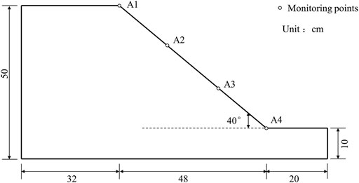
FIGURE 1. Slope dimension and monitoring point locations.

FIGURE 2

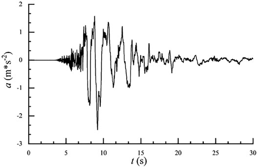
FIGURE 2. Acceleration time series of KOBE wave.

TABLE 1

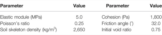
TABLE 1. Table of parameters in SPH simulation of the model test.

Figure 3 shows a comparison of the PGA amplification coefficient between the SPH simulation and the model test. At the elevation of 10 cm, the amplification coefficient of PGA obtained by SPH simulation is around 1.2, which is slightly smaller than 1.4 in the model test. In addition, both the PGA amplification coefficient increases with the height and the PGA amplification coefficient of the SPH simulation is increased from 1.2 to 2.0, which is close to the model test. Although the results of the numerical simulation have a few differences from the results of the test, which is because the soil model used in the SPH simulation is the elastic model, the PGA amplification coefficient of the slope at the top is close to 2.0, which is consistent with existing research studies [38–40]. Therefore, the method in this article can well-input the ground motion and analyze the dynamic response of soil slope.

FIGURE 3

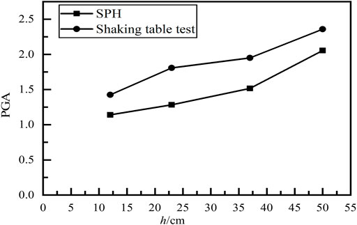
FIGURE 3. Comparison of PGA amplification coefficient between SPH simulation and the model test.

Validation of the Slope Deformation Under the Earthquake

In order to validate the applicability of the dynamic SPH method in the deformation analysis of soil slope, it is applied to a shaking table test, and the results are compared with the test results [41].

The total number of particles in the numerical model was 6,977, with 2,118 boundary particles and 4,857 soil particles. The initial spacing of the particles was 0.01 m. Meanwhile, the left boundary is set to the free-field boundary. At the initial stage, the soil slope is still and begins to move under the action of gravity and earthquake. The incremental time in the SPH simulation is 2.5 × 10^–5 s, and the total steps are 1.21 × 10⁷; thus, the total time is 302.5 s. In this simulation, the time for the generation of initial geostatic stress is set as 1 s, and the applying time of ground vibration is 300 s. In addition, after the application of ground vibration, the slope model is still moving, and it takes 1.5 s for the slope to reach the static state. The model parameters are shown in Table 2. Figure 4 shows the final deposit form between the SPH simulation and the shaking table test. The final shapes are basically consistent, and the maximum sliding distance of SPH simulation is very close to the test result. Therefore, the method in this article has high accuracy in the deformation analysis of soil slope under vibration loads.

TABLE 2

TABLE 2. Table of parameters in SPH simulation of a soil slope vibration table test.

FIGURE 4

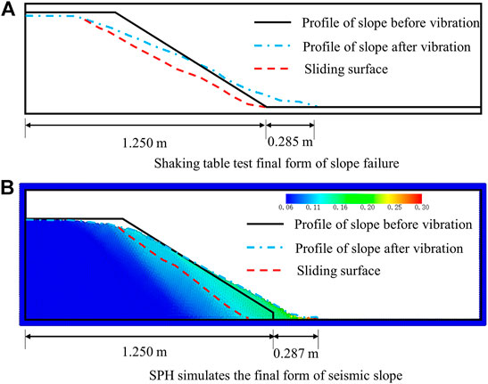
FIGURE 4. Final shape comparison of slope (unit: m).

Application Example—Dynamic Analysis of Soil Slopes With Different Slope Angles

Simulating Case

In order to analyze the sliding material volume and the influence range of soil slope failure with different angles under the action of the earthquake, this section shows four conceptual soil slopes with different angles, including 30°, 40°, 50°, and 60°. The simulating cases are shown in Table 3. The slope size is shown in Figure 5, and the locations of fixity boundary particles and free-field boundary particles are also shown in Figure 5. The safety factors of each slope calculated by the stability analysis method are all greater than 1.0, that is, each slope can remain stable under gravity. In this part, the total number of particles changes with slope angles, and the initial spacing of particles is uniformly set as 0.20 m. At the initial stage, the soil slope particles are stationary and can move under the action of gravity and earthquake after the calculation begins. The incremental time spacing in the SPH simulation was 5.0 × 10^–5 s, the total number of steps is 6.4 × 10⁵ steps, and the simulation time was 32 s. In this simulation, the time for the generation of initial geostatic stress is set as 1 s, and the applying time of ground vibration is 30 s. In addition, after the application of ground vibration, the slope model is still moving, and it takes 1 s for the slope to reach the static state. As a summary, the calculation parameters are shown in Table 4.

TABLE 3

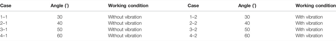
TABLE 3. Table of SPH simulating cases of conceptual slope.

FIGURE 5

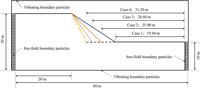
FIGURE 5. Size chart of different slopes.

TABLE 4

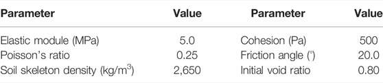
TABLE 4. Table of parameters in SPH simulation of soil slopes.

In the simulation, the geostatic stress is generated by the elastic model within 1.00 s, and thereafter, the behavior of soil is described by the Drucker–Prager model. Here, the KOBE wave as shown in Figure 2 is used for the dynamic analysis, and the loading time is 30 s, from 1.00 to 31.00 s. It takes about 2.0 h to complete a simulation using 16 threads on the same computing platform as in the previous section.

Discussion of Sliding Material Volume and Influence Range

The SPH simulations obtained the deformation of slopes with different angles under static and seismic conditions. Due to space limitation, Figure 6 only shows the total displacement distributions of slopes with 40° and 60°. It can be seen that each slope has no obvious displacement under the geostatic condition. Under the action of the earthquake, the slope surface has obvious deformation and eventually forms an obvious slip surface. In addition, with the increase of slope angle, the total displacement also increases, so with the same soil parameters, the greater the slope angle, the worse the stability.

FIGURE 6

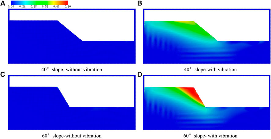
FIGURE 6. Horizontal deformation diagram of 40°and 60°slopes with or without vibration (unit: m).

At present, the shear strain is commonly used to determine the potential slip surface, while Li et al. [7] have checked the accuracy of using a displacement threshold to determine the slip surface of the slope. Herein, this study compares the potential slip surfaces of 40° and 60° slopes under the seismic action determined by shear strain and total displacement, as shown in Figure 7. The potential slip surface of the slope determined by the maximum shear strain has a certain degree of coincidence with the potential slip surface determined by the total displacement. The slip surface starts from the toe of the slope, and the sliding surface area determined by the two is similar. Therefore, it is proved once again that the displacement threshold can be used to determine the potential slip surface of soil slope.

FIGURE 7

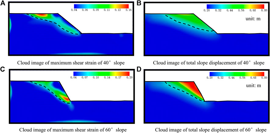
FIGURE 7. Cloud image of shear strain and a total displacement of 40° and 60° slope with vibration.

In addition, 0.10, 0.20, 0.30, and 0.40 m are selected as the displacement thresholds in this study. By simplifying the deformation distribution map with the displacement threshold, a clearer distribution of the slide material can be obtained. Figure 8 shows the sliding material volume of each slope with a displacement threshold of 0.20 m, which indicates that each slope has an obvious and regular sliding material volume.

FIGURE 8

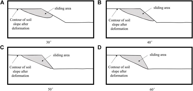
FIGURE 8. Sliding material volume comparison when the threshold is 0.20 m.

Then, the sliding material volume of each slope under different displacement thresholds is calculated in detail, and the change curve of sliding material volume with slope angles was drawn, as presented in Figure 9. It can be seen that the potential sliding volume will decrease with the increase of slope angles at a small displacement threshold, but the potential sliding volumes are very close. Under the larger displacement threshold, the sliding area will increase with the increase of slope angles, but the increase is very slow. The sliding material volume decreases greatly with the increase of slope angles, but the potential sliding volume of the 60° slope still increases with a larger displacement threshold.

FIGURE 9

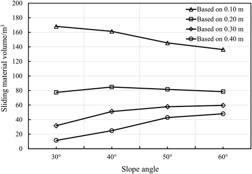
FIGURE 9. Sliding material volume change curves of slopes with slope angles under different deformation thresholds (The longitudinal length of the slope is assumed to be 1.00 m).

The maximum horizontal displacement of soil slope is regarded as the sliding distance of soil slopes under an earthquake, namely, the influence range, and the variation curve of influence range with slope angles is plotted in Figure 10. It can be seen that the influence range of soil slope increases linearly with the slope angle, and the angle has a significant effect on the sliding distance.

FIGURE 10

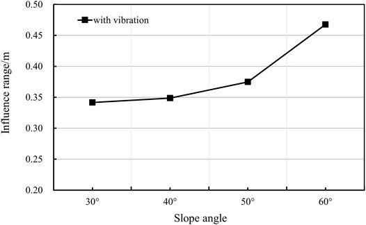
FIGURE 10. Change curves of the influence range of slopes with slope angles.

Conclusion

In this study, a dynamic SPH method is applied to a model test and a shaking table test of soil slopes in literature. By setting slopes of different angles and comparing the results of SPH simulation with or without an earthquake, the sliding material volume and influence range of soil slope under the action of the earthquake are analyzed, and the relationships between sliding material volume, influence range, and slope angle are obtained and discussed. Some conclusions can be derived as follows:

1) The acceleration time history and PGA amplification coefficient obtained from the dynamic SPH simulation are compared with the test results, which proves that the proposed dynamic SPH method can be used to analyze the dynamic response of soil slope.

2) Aiming at the deformation analysis of soil slope under earthquakes, the SPH simulation results of a shaking table test are compared with the test results, and the proposed method can be applied to the deformation analysis of slope under earthquakes.

3) In the analysis of sliding material volume under different slope angles, the sliding volume of the slope will decrease with the increase of slope angles at a small displacement threshold, but the sliding material volume of each slope is very similar. At the larger displacement threshold, the sliding material volume will increase with the increase of slope angles, but the increase is very slow.

4) In the analysis of influence range with different slope angles, the maximum horizontal displacement of slope under earthquakes presents a trend of nonlinear increase with the increase of slope angles.

Data Availability Statement

The original data presented in the study are all included in the article and further inquiries can be directed to the corresponding author.

Author Contributions

WZ wrote, checked, and revised this manuscript. RY wrote and revised this manuscript. YC provided revision recommendations for this manuscript. SC provided revision recommendations for this manuscript.

Funding

This study was supported by the National Natural Science Foundation of China (No. 51808192), the Fundamental Research Funds for the Central Universities (Grant No. B210202039), and the Natural Science Foundation of Jiangsu Province (No. BK20211575).

Conflict of Interest

The authors declare that the research was conducted in the absence of any commercial or financial relationships that could be construed as a potential conflict of interest.

Publisher’s Note

All claims expressed in this article are solely those of the authors and do not necessarily represent those of their affiliated organizations, or those of the publisher, the editors, and the reviewers. Any product that may be evaluated in this article, or claim that may be made by its manufacturer, is not guaranteed or endorsed by the publisher.

References

1. Huang RQ. Mechanism and Geomechanical Modes of Landslide Hazards Triggered by Wenchuan 8.0 Earthquake. Chin J Rock Mech Eng (2008) 28(6):1239–49. doi:10.1002/9780470611807.ch2

CrossRef Full Text | Google Scholar

2. Hu XW, Huang RQ, Shi YB, Lv XP, Zhu HY, Wang XR. Analysis of Blocking River Mechanism of Tangjiashan Landslide and Dam-Breaking Mode of its Barrier Dam. J Hohai Univ (Natural Sciences) (2009) 28(1):181–9. CNKI:SUN:YSLX.0.2009-01-027.

Google Scholar

3. Yin Y, Wang F, Sun P. Landslide Hazards Triggered by the 2008 Wenchuan Earthquake, Sichuan, China. Landslides (2009) 6(2):139–52. doi:10.1007/s10346-009-0148-5

CrossRef Full Text | Google Scholar

4. Xu Q, Huang RQ. Kinetics Charateristics of Large Landslides Triggered by May 12th Wenchuan Earthquake. J Eng Geology (2008) 16(6):721–9. doi:10.3969/j.issn.1004-9665.2008.06.001

CrossRef Full Text | Google Scholar

5. Xu C, Tang XB, Wang SY, Xu XW, Zhang H, Tian YY, et al. A Panorama of Landslides Triggered by the 8 August 2017 Jiuzaigou, Sichuan MS7.0 Earthquake. Seismology Geology (2018) 40(01):232–60. doi:10.3969/j.issn.0253-4967.2018.01.017

CrossRef Full Text | Google Scholar

6. Bao Y, Huang Y, Liu GR, Wang G. SPH Simulation of High-Volume Rapid Landslides Triggered by Earthquakes Based on a Unified Constitutive Model. Part I: Initiation Process and Slope Failure. Int J Comput Methods (2020) 17(04):1850150–890. doi:10.1142/S0219876218501505

CrossRef Full Text | Google Scholar

7. Li L, Wang Y. Identification of Failure Slip Surfaces for Landslide Risk Assessment Using Smoothed Particle Hydrodynamics. Georisk: Assess Manag Risk Engineered Syst Geohazards (2020) 14(2):91–111. doi:10.1080/17499518.2019.1602877

CrossRef Full Text | Google Scholar

8. Wu Y, Liu DS, Zhou ZH. Mobility Assessment Model for Landslide Mass Considering Disintegration Energy Consumption in Slipping Process. Chin J Geotechnical Eng (2015) 37(01):35–46. doi:10.11779/CJGE201501003

CrossRef Full Text | Google Scholar

9. Burridge R, Knopoff L. Model and Theoretical Seismicity. Bull Seis Soc Amer (1967) 57(3):341–71. doi:10.1785/bssa0570030341

CrossRef Full Text | Google Scholar

10. Parteli E, Gomes M, Montarroyos E, Brito VP. Omori Law for Slidings of Blocks on Inclined Rough Surfaces. Physica A: Stat Mech its Appl (2001) 292(1-4):536–44. doi:10.1016/S0378-4371(00)00629-4

CrossRef Full Text | Google Scholar

11. Zhou Y, Zhang F, Wang J, Gao Y, Dai G. Seismic Stability of Earth Slopes with Tension Crack. Front Struct Civ Eng (2019) 13(4):950–64. doi:10.1007/s11709-019-0529-3

CrossRef Full Text | Google Scholar

12. Xia ZX, Li P, Cao B, Li T, Shen W, Kang H. Bayesian Estimation and Posterior Robustness of Slope Reliability. J Hohai Univ (Natural Sciences) (2020) 48(3):238–44. doi:10.3876/j.issn.1000-1980.2020.03.008

CrossRef Full Text | Google Scholar

13. Yin X, Wang L. Block Limit Analysis Method for Stability of Slopes during Earthquakes. J Shanghai Jiaotong Univ (Sci.) (2018) 23(6):764–9. doi:10.1007/s12204-018-1997-7

CrossRef Full Text | Google Scholar

14. Zhou Z, Zhang F, Gao Y-f., Shu S. Nested Newmark Model to Estimate Permanent Displacement of Seismic Slopes with Tensile Strength Cut-Off. J Cent South Univ (2019) 26(7):1830–9. doi:10.1007/s11771-019-4137-0

CrossRef Full Text | Google Scholar

15. Cui Y, Liu A, Xu C, Zheng J. A Modified Newmark Method for Calculating Permanent Displacement of Seismic Slope Considering Dynamic Critical Acceleration. Adv Civil Eng (2019) 2019(3):1–10. doi:10.1155/2019/9782515

CrossRef Full Text | Google Scholar

16. Li K, Chen GR. Finite Element Analysis of Slope Stability Based on Theory of Slip Line Field. J Hohai Univ (Natural Sciences) (2010) 38(2):191–5. doi:10.3876/j.issn.1000-1980.2010.02.014

CrossRef Full Text | Google Scholar

17. Wang L, Li N, Wang P, Wang H. Study on Dynamic Stability of High-Steep Loess Slope Considering the Effect of Buildings. Soil Dyn Earthquake Eng (2020) 134:106146. doi:10.1016/j.soildyn.2020.106146

CrossRef Full Text | Google Scholar

18. Zhao L, Huang Y, Chen Z, Ye B, Liu F. Dynamic Failure Processes and Failure Mechanism of Soil Slope under Random Earthquake Ground Motions. Soil Dyn Earthquake Eng (2020) 133:106147–7. doi:10.1016/j.soildyn.2020.106147

CrossRef Full Text | Google Scholar

19. Mao Z, Liu GR, Huang Y. A Local Lagrangian Gradient Smoothing Method for Fluids and Fluid-like Solids: A Novel Particle-like Method. Eng Anal boundary Elem (2019) 107:96–114. doi:10.1016/j.enganabound.2019.07.003

CrossRef Full Text | Google Scholar

20. Cuomo S, Pastor M, Capobianco V, Cascini L. Modelling the Space-Time Evolution of Bed Entrainment for Flow-like Landslides. Eng Geology (2016) 212:10–20. doi:10.1016/j.enggeo.2016.07.011

CrossRef Full Text | Google Scholar

21. Huang Y, Zhang W, Xu Q, Xie P, Hao L. Run-out Analysis of Flow-like Landslides Triggered by the Ms 8.0 2008 Wenchuan Earthquake Using Smoothed Particle Hydrodynamics. Landslides (2012) 9(2):275–83. doi:10.1007/s10346-011-0285-5

CrossRef Full Text | Google Scholar

22. Huang Y, Dai Z. Large Deformation and Failure Simulations for Geo-Disasters Using Smoothed Particle Hydrodynamics Method. Eng Geology (2014) 168(1):86–97. doi:10.1016/j.enggeo.2013.10.022

CrossRef Full Text | Google Scholar

23. He X, Liang D, Bolton MD. Run-out of Cut-Slope Landslides: Mesh-free Simulations. Géotechnique (2018) 68(1):50–63. doi:10.1680/jgeot.16.P.221

CrossRef Full Text | Google Scholar

24. Chen W, Qiu T. Simulation of Earthquake-Induced Slope Deformation Using SPH Method. Int J Numer Anal Meth Geomech (2014) 38(3):297–330. doi:10.1002/nag.2218

CrossRef Full Text | Google Scholar

25. Bao Y, Huang Y, Liu GR, Zeng W. SPH Simulation of High-Volume Rapid Landslides Triggered by Earthquakes Based on a Unified Constitutive Model. Part II: Solid-liquid-like Phase Transition and Flow-like Landslides. Int J Comput Methods (2020) 17(04):1850149. doi:10.1142/S0219876218501499

CrossRef Full Text | Google Scholar

26. Huang Y, Dai ZL, Zhang WJ. Geo-disaster Modeling and Analysis: An SPH-Based approach[M]. Berlin: Springer (2014).

Google Scholar

27. Zhang W, Zheng H, Jiang F, Wang Z, Gao Y. Stability Analysis of Soil Slope Based on a Water-Soil-Coupled and Parallelized Smoothed Particle Hydrodynamics Model. Comput Geotechnics (2019) 108:212–25. doi:10.1016/j.compgeo.2018.12.025

CrossRef Full Text | Google Scholar

28. Zhang W, Maeda K, Saito H, Li Z, Huang Y. Numerical Analysis on Seepage Failures of dike Due to Water Level-Up and Rainfall Using a Water-Soil-Coupled Smoothed Particle Hydrodynamics Model. Acta Geotech. (2016) 11(6):1401–18. doi:10.1007/s11440-016-0488-y

CrossRef Full Text | Google Scholar

29. Huang Y, Zhang W, Dai Z, Xu Q. Numerical Simulation of Flow Processes in Liquefied Soils Using a Soil-Water-Coupled Smoothed Particle Hydrodynamics Method. Nat Hazards (2013) 69(1):809–27. doi:10.1007/s11069-013-0736-5

CrossRef Full Text | Google Scholar

30. Bui HH, Fukagawa R. An Improved SPH Method for Saturated Soils and its Application to Investigate the Mechanisms of Embankment Failure: Case of Hydrostatic Pore-Water Pressure. Int J Numer Anal Meth Geomech (2013) 37:31–50. doi:10.1002/nag.1084

CrossRef Full Text | Google Scholar

31. Peng C, Guo X, Wu W, Wang Y. Unified Modelling of Granular media with Smoothed Particle Hydrodynamics. Acta Geotech. (2016) 11(6):1231–47. doi:10.1007/s11440-016-0496-y

CrossRef Full Text | Google Scholar

32. Bui HH, Sako K, Fukagawa R. Numerical Simulation of Soil-Water Interaction Using Smoothed Particle Hydrodynamics (SPH) Method. J Terramechanics (2007) 44(5):339–46. doi:10.1016/j.jterra.2007.10.003

CrossRef Full Text | Google Scholar

33. Peng C, Wang S, Wu W, Yu H-s., Wang C, Chen J-y. LOQUAT: an Open-Source GPU-Accelerated SPH Solver for Geotechnical Modeling. Acta Geotech. (2019) 14(5):1269–87. doi:10.1007/s11440-019-00839-1

CrossRef Full Text | Google Scholar

34. Hiraoka N, Oya A, Rajeev P, Fukagawa R. Seismic Slope Failure Modelling Using the Mesh-free SPH Method. Int J GEOMATE (2013) 5(1):660–5. doi:10.21660/2013.9.3318

CrossRef Full Text | Google Scholar

35. Zhang WJ, Zheng H, Wang ZB, Gao YF. Study on Flowing Behavior of Soil Based on Three Dimensional and Parallelized SPH Model. J Eng Geology (2018) 26(5):1279–84. doi:10.13544/j.cnki.jeg.2018114

CrossRef Full Text | Google Scholar

36. Zhang WJ, Gao YF, Huang Y, Maeda K. Normalized Correction of Soil-Water-Coupled SPH Model and its Application. Chin J Geotechnical Engineer (2018) 40(2):262–9. doi:10.11779/CJGE201802006

CrossRef Full Text | Google Scholar

37. Tang WM, Ma SZ, Liu XL, Zhao X. Influence of Topographic and Geomorphic Conditions on the Dynamic Response of Slope Acceleration. J Yangtze River Scientific Res Inst (2019) 36(11):98–103. doi:10.11988/ckyyb.20180443

CrossRef Full Text | Google Scholar

38. Sun Z, Kong L, Guo A, Xu G, Bai W. Experimental and Numerical Investigations of the Seismic Response of a Rock-Soil Mixture deposit Slope. Environ Earth Sci (2019) 78(24):716. doi:10.1007/s12665-019-8717-y

CrossRef Full Text | Google Scholar

39. Sun Z, Kong L, Guo A, Alam M, Mohammad A. Centrifuge Model Test and Numerical Interpretation of Seismic Responses of a Partially Submerged deposit Slope. J Rock Mech Geotechnical Eng (2020) 12(2):381–94. doi:10.1016/j.jrmge.2019.06.012

CrossRef Full Text | Google Scholar

40. Huang Q, Jia X, Peng J, Liu Y, Wang T. Seismic Response of Loess-Mudstone Slope with Bedding Fault Zone. Soil Dyn Earthquake Eng (2019) 123:371–80. doi:10.1016/j.soildyn.2019.05.009

CrossRef Full Text | Google Scholar

41. Huang D, Qiao JP, Zhang XG, Chen YL. Experimental Research of the Topographic Effects of Slopes in Earthquake. Chin J Rock Mech Eng (2017) 36(3):587–98. doi:10.13722/j.cnki.jrme.2016.0952

CrossRef Full Text | Google Scholar