Dynamic Interactions of Multiple Wall-Mounted Flexible Plates in a Laminar Boundary Layer

The interactions between large arrays of wall-mounted flexible plates and oncoming laminar boundary-layer flows are studied numerically by using the immersed boundary method. The influences of bending rigidity, mass ratio and gap distance between adjacent plates on the dynamic behaviors are explored. With the variation of control parameters, five distinct dynamic modes, namely, static reconfiguration, sectional waving, regular waving, upright oscillation and cavity oscillation, are identified. The frequency lock-in phenomenon and various types of flow instability associated with different dynamic modes are discussed. The findings of this study indicate that the coherent motions of the arrays are governed by a coupled mechanism in which the frequency of flow instability is locked onto the structural natural frequency.

1 Introduction

The motion of wall-mounted flexible structures in fluid flow is a phenomenon that is commonly observed in nature. Some well-known examples include: tree and wheat swaying in the wind, reed and seaweed waving in the current, cilia beating in the bronchial tube. These systems are inherently mulitphysics and involve fluid-structure interaction (FSI). The study of this subject is not only important to scientific progress but also inspires engineering innovations in a variety of disciplines such as flow control, flow sensing, energy harvesting and heat transfer enhancement.

Theoretical, experimental and numerical approaches have been used to investigate simplified models to gain a better understanding of the flow physics behind such phenomenon. The models often used in the studies included: 1D plates (filaments) exposed to a 2D transverse flow, 2D plates (or cylindrical beams) exposed to a 3D transverse flow. Please note that the words for describing the slender structures were sometimes interchangeable in the literature, e.g., beam, flap, filament, plate, membrane, panel, flag, etc.

In some theoretical studies, the fluid load on the structure was estimated by reduced-order models. Luhar and Nepf [1] considered the effect of flow-induced static reconfiguration on the scaling law between drag and velocity in a model blade. In the work by Leclercq and de Langre [2], it was found that a flexible beam can always enjoy drag reduction when subjected to a steady transverse flow, either in static reconfiguration or in fluttering. The effects of oscillatory transverse flow [3] or non-uniform transverse flow and non-uniform material property [4, 5] on the reconfiguration of the beam were also explored in other works.

Jin and coauthors [6–9] conducted a series of experiments to explore the FSI behaviors of flexible wall-mounted plates subjected to turbulent transverse flow in the Reynolds number range of 10⁴–10⁵. In Jin et al. [6], it was reported that under certain circumstances, the frequencies for the oscillating structures and wake fluctuations can by significantly decoupled. In Jin et al. [7], the influences of tip shape on the dynamics of the plate and near wake turbulence were investigated. In Jin et al. [8], the existence of three distinctive modes of tip oscillations were reported in wall-mounted flexible plates under various inclined flows. In Jin et al. [9], the coupled dynamics of two flexible plates in tandem arrangement was explored. It was found that the upstream plate always oscillated at its natural frequency, while oscillation of the downstream one was significantly influenced by the vortices shed from the upstream structure.

On the numerical side, simulations have been conducted to explore the FSI behaviors of vertically clamped 1D filaments [10, 11] and 2D flexible plates (flags) [12] subjected to laminar oncoming flows. Zhang et al. [10] systematically studied the kinematic states and frequency lock-in mechanisms in the interactions of single- and dual-filament systems with a laminar boundary-layer flow. Three dynamic modes, namely, lodging, static reconfiguration and regular VIV, were identified in the single-filament system. In additional to the three modes aforementioned, a distinctive mode termed “cavity oscillation” was also observed in the dual-filament system. In a similar study by Wang et al. [11], the interactions of single-, dual- and triple-filament systems with an oncoming Poiseuille flow were studied. The influences of bending rigidity and gap distance on the dynamic modes and vortical structures were revealed. Chen et al. [12] extended the work by Wang et al. [11] by conducting three-dimensional simulations to study the FSI of a single flag and dual flags in a Poiseuille flow.

If large numbers of wall-mounted flexible structures are organized into an array, the interactions with fluid flow can give rise to coherent waving motions. This type of collective motions is widely observed in canopies of terrestrial or aquatic plants. Such phenomenon is known as honami for terrestrial plants, and monami for aquatic plants [13, 14]. It is generally accepted that the mixing layer instability [15–17] is one primary cause of the coherent waving motion. However, it was also argued in some studies that the elastic properties of the flexible structures may also play an essential role in the development of coherent waving motion [18–20]. It should be noted that in the works above, the canopy was modeled as a flexible porous layer and the fluid flow around individual plants was not fully resolved. In a recent study by Wong et al. [21], the canopy was modeled as a collection of homogeneous elastic beams. The steady configuration of the canopy under a unidirectional flow was predicted by coupling the beam equations with the Navier-Stokes equations. A linear stability analysis was then conducted to identify the dominant factors that determined the onset of instability. O’Conner and Revell [22] performed FSI simulations on a large array of slender structures placed in a steady open-channel flow. In their work, a lattice Boltzmann-immersed boundary method was used and the flow around individual structures was fully resolved. Their findings indicated that the coherent waving motion was triggered by a coupled instability, in which the fluid oscillation frequency was locked onto the structural natural frequency. More recently, the dynamic response of a shallow submerged vegetation canopy in an open-channel flow at the Reynolds number of 100 was studied numerically by Fang et al. [23]. The vortical structures in the developed mixing layer were investigated in detail, and the lock-in between frequency of mixing layer instability and natural frequency was also observed.

Despite of the fruitful insights gained in the previous works, the coupled dynamics and FSI behaviors of multiple wall-mounted flexible structures are far from being fully understood. For instance, in a preliminary investigation of our group, it was found that the dynamic behaviors of the structures in different portions of the array may differ significantly. Furthermore, the dynamic interactions of the flexible structures in the array may be greatly influenced by the gap distance between adjacent structures. The phenomena above and associated physical mechanisms have never been thoroughly explored in the previous works.

In the present study, numerical simulations are performed to systematically investigate the interactions of large arrays of flexible 1D plates (filaments) with a 2D laminar boundary-layer flow. Several distinct modes for characterizing the dynamic behaviors of the system are identified. The influences of bending rigidity, mass ratio and gap distance on the dynamic behaviors are also explored. The frequency lock-in phenomenon and various types of flow instability involved are discussed. The physical mechanisms associated with different dynamic modes are elucidated.

The rest of the paper is organized as follows. The computational model is described in section 2. The numerical methods and computational configurations are introduced in section 3. The results and discussion are presented in section 4. Finally, the conclusions are drawn in section 5.

2 Computational Model

In the present study, we consider FSI of a large array of multiple flexible plates with an oncoming laminar boundary-layer flow. The schematic diagram of the computational model is shown in Figure 1A. An array of wall-mounted flexible plates is vertically clamped on the bottom wall. The number of plates in the array is n. The plates are of length L and are equally spaced by a distance of D. The inclination angle θ is defined as the angle between the chord line and the horizontal axis. A uniform velocity of U_∞ is prescribed at the left entrance, and a laminar boundary layer is developed along the bottom wall. D₁ denotes the distance between the entrance and the first plate. In the present study, D₁ is set to 8L.

FIGURE 1

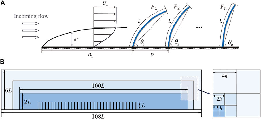
FIGURE 1. (A) A Schematic diagram of the computational model. (B) A schematic diagram of the computational domain and the multi-block Cartesian mesh.

The incompressible Navier-Stokes equations which govern the fluid flow can be written in a dimensionless form as

$\frac{\partial \mathit{u}}{\partial t}+\left(\mathit{u}\cdot \nabla \right)\mathit{u}=-\nabla p+\frac{1}{Re}{\nabla }^2\mathit{u}+\mathit{f},(\mathrm{1a})$

$\nabla \cdot \mathit{u}=0,(\mathrm{1b})$

where u is the velocity of the fluid flow, p is the pressure, and f is the Eulerian force which represents the effect of immersed objects on the fluid. The Reynolds number Re is defined as U_∞L/ν, where ν is the kinematic viscosity of the fluid.

The dynamic equations which govern the motions of the flexible plates can be written in a dimensionless form as

$\beta \frac{{\partial }^2\mathit{X}}{\partial t^2}-\frac{\partial }{\partial s}\left(\zeta \frac{\partial \mathit{X}}{\partial s}\right)+\frac{{\partial }^2}{{\partial }^{2}s}\left(\gamma \frac{{\partial }^2\mathit{X}}{\partial s^2}\right)=-\mathit{F}+{\mathit{F}}_{\mathit{c}},(\mathrm{2a})$

$\frac{\partial \mathit{X}}{\partial s}\cdot \frac{\partial \mathit{X}}{\partial s}=1,(\mathrm{2b})$

where X = X (s, t) is the position vector of the Lagrangian points (s is the Lagrangian coordinate along the arc length). F is the Lagrangian force which represents the interaction between the structure and the flow. F_c is an artificial short-range repulsive force which is added to avoid the collisions between adjacent plates (and between the plates and the wall). The repulsive force can be formulated by using the discrete delta function as [10, 11, 24].

${\mathit{F}}_c\left(s,t\right)=c_1\cdot \sum _k{\int }_0^L{\delta }_h\left(\mathit{X}\left(s,t\right)-{\mathit{X}}_k^{\prime }\left(s^{\prime },t\right)\right)\frac{\mathit{X}-{\mathit{X}}_k^{\prime }}{\left|\mathit{X}-{\mathit{X}}_k^{\prime }\right|}d{s}^{\prime }+c_2\cdot {\delta }_h\left(\mathit{X}\left(s,t\right)-{\mathit{X}}_p\left(s,t\right)\right)\mathit{j},(3)$

where δ_h represents the discrete Delta function. In the present work, the three-point discrete Delta function [25] is used. ${\mathit{X}}_k^{\prime }(s^{\prime },t)$ denotes the position vector of the Lagrangian points on one adjacent plate. Here k is the index of the adjacent plate and s′ is the arc length along the plate. $\sum _k$ denotes the summation over adjacent plates. X_p is the projection of X on the wall. j is the unit normal vector on the wall. The first term on the right-hand side of Eq. (3) denotes the repulsive force between adjacent plates, while the second term represents the repulsive force between the plate tip and the wall. c₁ and c₂ represent the adjustable constants. The values of the two constants are chosen such that the minimal repulsive force is exerted to prevent the plates from penetrating into each other or penetrating into the wall. It is found that c₁ = 1.0 and c₂ = 1.0 can yield satisfactory results by ensuring that the smallest plate-plate distance and tip-wall distance are never less than one grid width. It should be noted that the smallest plate-plate distance and tip-wall distance are not sensitive to the values of c₁ and c₂. The dynamic behaviors of the plates are almost not affected by the magnitude of F_c (at least for certain ranges of c₁ and c₂ with c₁ ≥ 1.0 and c₂ ≥ 1.0).

β, ζ, γ represent the mass ratio, the dimensionless tension coefficient and the dimensionless bending rigidity, respectively. The definitions of the three dimensionless quantities are:

$\beta =\frac{{\rho }_s\delta }{{\rho }_{f}L},\zeta =\frac{T}{{\rho }_f{U}_{\infty }^{2}L},\gamma =\frac{B}{{\rho }_f{U}_{\infty }^2{L}^3},(4)$

where ρ_s and ρ_f are the densities of the structure and the fluid, respectively. δ is the thickness of the plate. T and B represent the dimensional tension coefficient and bending rigidity, respectively. The inhomogeneous tension coefficient ζ in Eq.(2a) introduces geometric nonlinearity to the structural model. It also acts as the Lagrange multiplier that enforces the inextensibility condition [Eq.(2b)].

3 Numerical Methods and Configurations

3.1 Flow and Structure Solvers

The incompressible Navier-Stokes equations Eqs (1a, 1b) are solved by using direct-forcing immersed boundary method based on the discrete stream-function formulation [26, 27]. In this approach, the discrete stream-function is treated as the primary unknown, while the continuity equation is exactly satisfied and the need for solving a pressure Poisson equation is eliminated [28]. The finite difference method is used for the spatial discretization of Eqs (2a, 2b) a three-time-level scheme is used for the temporal advancement. The inhomogeneous tension coefficient ζ can be determined by solving a linear boundary value problem, in which the governing equation for ζ is derived by rearranging Eqs (2a, 2b) [24]. A loosely coupled scheme, in which the fluid equations and the structural equations are advanced sequentially, is used for the FSI simulation of the present work. The massage passing interface (MPI) protocol is used for the parallelization of the FSI code [29]. This code has been extensively validated in previous studies, such as self-propulsion of fish-like elastic filaments [30, 31] and FSI of single and dual wall-mounted flexible filaments [10].

3.2 Numerical Configuration

The computational domain is of rectangular shape with the dimensions of [0, 108L] × [0, 6L]. A multi-block Cartesian mesh with hanging nodes is employed in the simulations (Figure 1B). In the vicinity of the structures, the finest grids with the width of 0.01 L are deployed in a subdomain of [6L, 100L] × [0, 2L] to capture the small wake structures. In the regions that are far away from the plates, the grid width ranges from 0.02L to 0.08L to reduce the total number of grid points. For the flexible structures, each plate is represented by 101 Lagrangian points with uniform spacing of 0.01 L. In addition, the dimensionless time steps used in the simulations are chosen such that the maximum Courant-Friedrichs-Lewy (CFL) number based on U_∞ and the finest grid width never exceeds 0.1.

The boundary and initial conditions for the fluid flow and the wall-mounted flexible plates are as follows. For the fluid flow, non-slip condition is imposed on the bottom boundary. Free-slip condition (with zero normal velocity and zero normal gradient of tangential velocity) is imposed on the top boundary. A uniform velocity is prescribed on the left boundary. The outflow condition with constant pressure is imposed on the right boundary. On the surface of the structures, non-slip boundary condition is enforced by using the direct-forcing immersed boundary technique. For the wall-mounted flexible plates, the boundary conditions at the free ends are:

$\frac{{\partial }^2\mathit{X}}{\partial s^2}={\left(\mathrm{0,0}\right)}^T,\frac{{\partial }^3\mathit{X}}{\partial s^3}={\left(\mathrm{0,0}\right)}^T.(5)$

The boundary conditions at the fixed ends are:

$\mathit{X}={\left(x_0,0\right)}^T,\frac{\partial \mathit{X}}{\partial s}={\left(\mathrm{0,1}\right)}^T.(6)$

The initial fluid velocity is set to U_∞ and all structures are vertically orientated initially (θ = 90°) and have zero velocity.

To ensure that the mesh resolution is sufficient for resolving the laminar boundary layer and small flow structures, mesh-sensitivity tests are systematically conducted in our previous work on FSI of single and dual wall-mounted flexible filaments in a laminar boundary layer [10]. Based on the experience gained in our previous work, the mesh resolution used in the present study is sufficient for obtaining accurate and mesh-independent results.

4 Results and Discussion

4.1 Control Parameters and Metrics of Dynamic Behaviors

The four dimensionless control parameters in the present study are: Reynolds number (Re), dimensionless bending rigidity (γ), mass ratio (β), and dimensionless gap distance (d = D/L). The ranges of the four control parameters used in the simulations are summarized in Table 1. As a result, the dimensionless momentum thickness of the boundary layer at the position of the first plate is around 0.1. These values of control parameters are largely comparable with those used in some previous works [10, 11, 22, 23]. Here the Reynolds number is chosen to be 400, which is much smaller than that in real vegetation flow (O (10⁵) or even higher). Such Reynolds number is close to the minimum value for generating waving instability (which is around 100 based on the study of O’Connor and Revell [22]). At such Reynolds number, the computational cost is not prohibitive, while the simulations are still relevant to the real vegetation canopy. The key metrics for quantifying the dynamic behaviors of wall-mounted plates are the mean inclination angle $(\bar{\theta })$ and the amplitude of angular oscillation (θ_A). These two quantities are defined as:

$\bar{\theta }=\frac{1}{\mathrm{\Delta }t}{\int }_{t_0}^{t_0+\mathrm{\Delta }t}\theta \left(t\right)dt,(\mathrm{7a})$

${\theta }_A={\theta }_{\mathit{max}}\left(t\right)-{\theta }_{\mathit{min}}\left(t\right),t_0\le t\le t_0+\mathrm{\Delta }t.(\mathrm{7b})$

TABLE 1

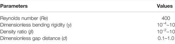
TABLE 1. Values of control parameters used in the simulations.

Here the lower limit in Eq. (7a) is chosen such that the periodicity of angular oscillation is fully established and the influence of initial condition becomes negligible (t₀ is set to 200 in the present work). The time interval Δt is chosen to be long enough such that the low-frequency waving motion can be captured (here Δt = 200 is considered to be sufficient). θ_max and θ_min in Eq.(7b) represent the maximum and minimum of the instantaneous inclination angle in t ∈ [t₀, t₀ + Δt], respectively.

In the present study, the number of plates in the array is set to 90. This number is sufficiently large such that the FSI behavior of the array remains largely unchanged if more plates are added. To test the influence of plate number on the FSI behavior, the distributions of mean inclination angle and oscillating amplitude along three arrays with 60, 90 and 120 plates are compared in Figure 2. As that shown in the figure, adding more plates to the array only affects $\bar{\theta }$ and θ_A in plates near the rear end of the original array. From Figure 2B, it is also seen that if the plate number is increased from 60 to 90, the growth rate (slope) of θ_A (with respect to the plate index) in the rear portion decreases drastically. However, if the plate number is increased from 90 to 120, the growth rate (slope) of θ_A in the rear portion almost remains unchanged. In view of the convergence behavior in the growth rate of θ_A observed in arrays with 90 and 120 plates, the number of plates is set to 90 in the simulations.

FIGURE 2

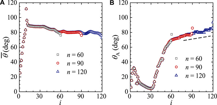
FIGURE 2. The distributions of mean inclination angle and amplitude of angular oscillation along the array for three arrays with different plate numbers. (A) Mean inclination angle, (B) amplitude of angular oscillation. The fixed control parameters are: γ = 0.02, β = 1.0, Re = 400 and d = 0.5.

4.2 Influences of Bending Rigidity and Mass Ratio on the Dynamic Behaviors

In this section, the influences of dimensionless bending rigidity and mass ratio on the dynamic behaviors of the arrays are systematically investigated. First, the influence of dimensionless bending rigidity is explored. To this end, γ is allowed to vary in a wide range as that listed in Table 1, while the rest of control parameters are kept fixed (β = 1.0, Re = 400, d = 0.5). With the variation of bending rigidity, several distinct dynamic modes of the array can be identified. The patterns of motion in the plates and wake structures for some selected cases corresponding to different dynamic modes are displayed in Figure 3.

FIGURE 3

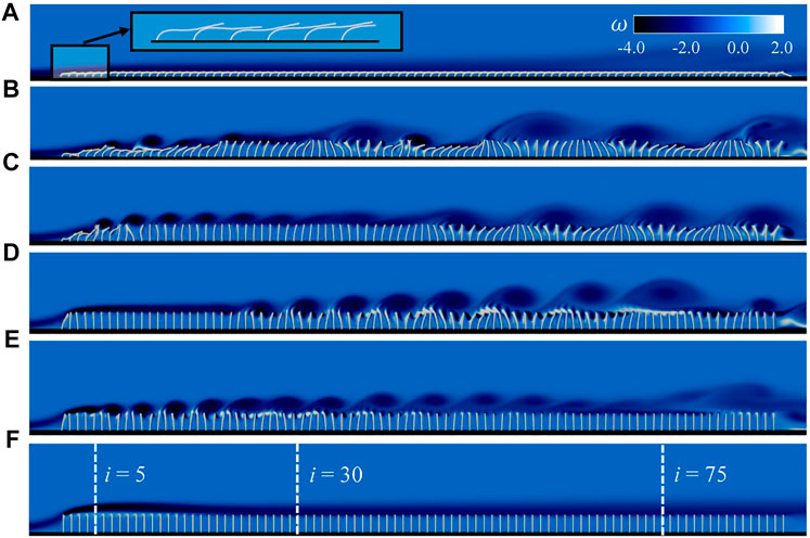
FIGURE 3. The patterns of motion and wake structures for some selected cases at various bending rigidities. (A) γ = 0.001 (static reconfiguration mode at extremely low rigidity, with a zoom-in view near the front), (B) γ = 0.01 (sectional waving mode with quasi-periodic oscillations), (C) γ = 0.02 (sectional waving mode with periodic oscillations), (D) γ = 0.2 (regular waving mode with periodic oscillations), (E) γ = 0.5 (upright oscillation mode), (F) γ = 10⁴ (static reconfiguration mode at extremely high rigidity). The fixed control parameters are: β = 1.0, Re = 400 and d = 0.5.

At an extremely low rigidity (γ = 10^–3), the static reconfiguration mode is observed (Figure 3A). All plates bend significantly backward and form an ‘end-to-end’ chain which is parallel to the wall. It should be noted that due to the existence of short-range repulsive forces, there is no direct contact (or collision) between adjacent plates. The angular oscillations of the plates are negligible and a long stable shear layer remains attached to the free ends.

With the increase of bending rigidity, three different dynamic modes with flow-induced oscillations emerge in turn. The sectional waving mode is observed at γ = 0.01 and γ = 0.02 (Figure 3B and Figure 3C). In the front portion of the array, vortices shed periodically from the free ends of some plates. This vortex shedding phenomenon resembles that in flow over a thin vertical plate. In the middle portion, due to the merging of vortices, the flow is stabilized and a shear layer on top of the plates appears. In the rear portion, due to the instability of the shear layer, vortices of much larger scale are produced on top of the array. Since the flow structures that drive the oscillations have much larger length scales than those in the front portion, the plates in this portion oscillate at a much lower frequency than those in the front portion. If we compare the two cases shown in Figure 3B and Figure 3C, more irregularities in the motions of the plates and the wake structures are found in the former one (especially in the front and rear portions of the array).

At γ = 0.2, the regular waving mode is exhibited (Figure 3D). In this mode, the oscillations of the plates in the front portion are completely suppressed, and a long stable shear layer is developed along the top of the array. Again, in the rear portion, large-scale vortical structures appear on top of the free ends due to instability of the shear layer. In the sectional and regular oscillation modes, the coherent waving motions induced by the large-scale vortical structures look very similar to that observed in the canopies of terrestrial and aquatic plants [15]. At γ = 0.5, the upright oscillation mode is exhibited (Figure 3E). In this mode, the long stable shear layer is not observed. Periodic vortex-shedding is triggered near the free ends of the fifth plate where the pinch-off of a short shear layer occurs. This phenomenon shares some similarities with that observed in flow over a rectangular cylinder with flat top. Since the strength of shed vortices attenuates very rapidly along the array, the oscillations in the rear portion become rather weak.

At an extremely high rigidity (γ = 10⁴), the static reconfiguration mode emerges again and the plates in the array stay upright (Figure 3F). A long stable shear layer remains attached to the free ends along the entire array and oscillations are completely suppressed.

To quantitatively characterize the behaviors of arrays with flow-induced oscillations, we show the distributions of mean inclination angle, envelope of angular oscillation, and dominant oscillating frequency for some cases in Figure 4. The time series of θ for two selected plates, i = 5 and i = 75 which represent the front and rear portions of the array, are also shown in the figure.

FIGURE 4

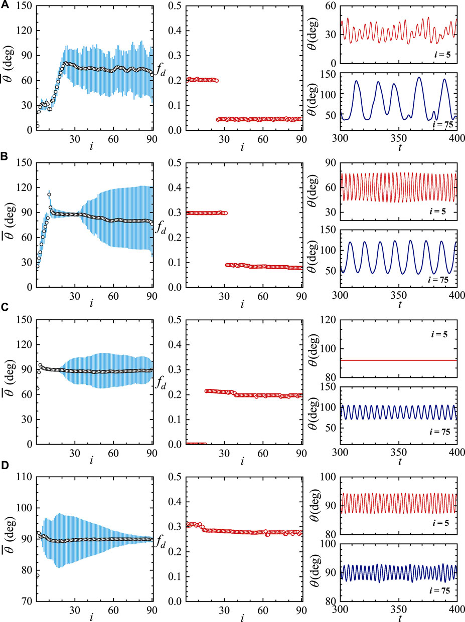
FIGURE 4. The distributions of mean inclination angle along the array (left column), the distributions of dominant frequency (f_d) along the array (middle column), and the time histories of inclination angles of the 5th and 75th plates (right column) for four selected cases. (A) γ = 0.01 (sectional waving mode with quasi-periodic oscillations), (B) γ = 0.02 (sectional waving mode with periodic oscillations), (C) γ = 0.2 (regular waving mode), (D) γ = 0.5 (upright oscillation mode). In the left column, the magnitude of oscillation amplitude is symbolized by the heights of cyan bars. The fixed control parameters are the same as those for Figure 3.

Figure 4A and Figure 4B show two cases (γ = 0.01 and γ = 0.02) of the sectional waving mode, respectively. Some similarities are shared by these two cases. In the front portion, the plates oscillate at a higher frequency but the amplitudes are rather small. In the rear portion, the plates oscillate at a lower frequency but with much larger amplitudes. The difference between these two cases lies in the time series of instantaneous inclination angles. In Figure 4A, quasi-periodicity is clearly visualized in the time series, while in Figure 4B, periodicity is exhibited in the time series. This can be further confirmed by comparing the normalized power spectra and phase diagrams spanned by θ and $\dot{\theta }$ (Figure 5). For the case of γ = 0.01, besides the dominant frequency, a lot of small peaks are also seen in the power spectra. The sectional waving mode with quasi-periodic oscillations can be regarded as a transitional state between the static reconfiguration mode and the sectional waving mode with periodic oscillations.

FIGURE 5

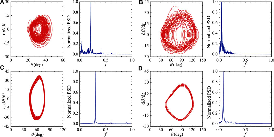
FIGURE 5. The phase diagrams and normalized power spectra of the angular oscillations of the 5th and 75th plates for two cases of the sectional waving mode. (A) γ = 0.01, i = 5 (quasi-periodic oscillation), (B) γ = 0.01, i = 75 (quasi-periodic oscillation), (C) γ = 0.02, i = 5 (periodic oscillation), (D) γ = 0.02, i = 75 (periodic oscillation). The fixed control parameters are the same as those in Figure 3.

Figure 4C shows one case of the regular waving mode (γ = 0.2). It is seen that the oscillations in the front portion are completely suppressed and periodic oscillations are observed in the rear portion. One case of the upright oscillation mode (γ = 0.5) is shown in Figure 4D. It is seen that the oscillating amplitude decreases steeply in the middle and rear portions. All plates in the array oscillate at almost the same frequency.

To further illustrate the characteristics of traveling wave propagation, the contours of inclination angles in the two-dimensional parametric space of plate index and time are shown in Figure 6. The selected cases are the same as those shown in Figure 4. In this figure, the oblique light (or dark) stripes represent the streamwise propagation of traveling waving along the array. The slope of the stripes signifies the speed of traveling, while the width of the light (or dark) stripes signifies oscillating frequency of the plates. In Figure 6A and Figure 6B, two different oscillating frequencies in the front and rear portions can be clearly seen. This is the prominent feature of the sectional waving mode. In Figure 6A, the attachment of slim branches on the stripes signifies quasi-periodicity in the oscillations of the rear portion. The black scribbles in the front portion signifies the effect of randomly activated repulsive force. In Figure 6C, the disappearance of oblique stripes in the front portion signifies the suppression of oscillations. The stripes with a uniform width in the rear portion signifies one single oscillating frequency. This is the prominent feature of the regular waving mode. In Figure 6D, stripes with a uniform width cover the entire region except a very narrow vertical band on the left margin. This indicates that almost all plates in the array (except very few at the front) oscillate at one single frequency. This is the prominent feature of the upright oscillation mode.

FIGURE 6

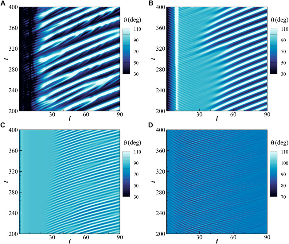
FIGURE 6. Contours of inclination angles in the space of plate index and time for some selected cases. (A) γ = 0.01 (sectional waving mode with quasi-periodic oscillations), (B) γ = 0.02 (sectional waving mode with periodic oscillations), (C) γ = 0.2 (regular waving mode), (D) γ = 0.5 (upright oscillation mode). Other control parameters are the same as those in Figure 3.

To determine the precise range of bending rigidity corresponding to each dynamics mode aforementioned, we examine the variations of $\bar{\theta }$ and θ_A with γ in the 5th and 75th plates (as shown in Figure 7). In this figure, the range of 10^–4 < γ < 3 × 10^–3 corresponds to the static reconfiguration mode. All plates fall over with a mean inclination angle of 15° and the oscillating amplitude is close to zero $(<1°)$. The mean inclination angle is much larger than that in the lodging mode of single-plate system reported in Zhang et al. [10], where $\bar{\theta }$ is approximately 0°. The larger inclination angle observed here is caused by the mutual repulsive force between adjacent plates. This force prevents the free ends of adjacent plates from approaching each other (and approaching the wall). The range of 3 × 10^–3 < γ < 0.09 corresponds to the sectional waving mode. The mean inclination angles of the two plates first increase sharply with increasing bending rigidity and then saturate (or slightly decrease). The huge “jumps” in these curves indicate the occurrence of a rapid transition in the motions of the plates. For example, near γ = 0.005, with increasing bending rigidity, the plates change from a nearly stationary state with large static deformation to a state with high-amplitude oscillation and nearly upright posture. It is also observed that the oscillating amplitude of the front plate is always much larger than that of the rear one (except in a narrow range of 3 × 10^–3 < γ < 5 × 10^–3). The range of 0.09 < γ < 0.5 corresponds to the regular waving mode. The mean inclination angles of the two plates are approximately 90°, which signifies a nearly upright posture. Oscillation is only observed in the rear plate, while oscillation in the front plate is completely suppressed. The range of 0.5 < γ < 1.0 corresponds to the upright oscillation mode. Both plates keep the upright posture $(\bar{\theta }\approx 90°)$ and oscillate with a very small amplitude. The range of γ > 1.0 corresponds to the reappearance of the static reconfiguration mode. Now both plates behave like a rigid structure and the oscillations are completely suppressed.

FIGURE 7

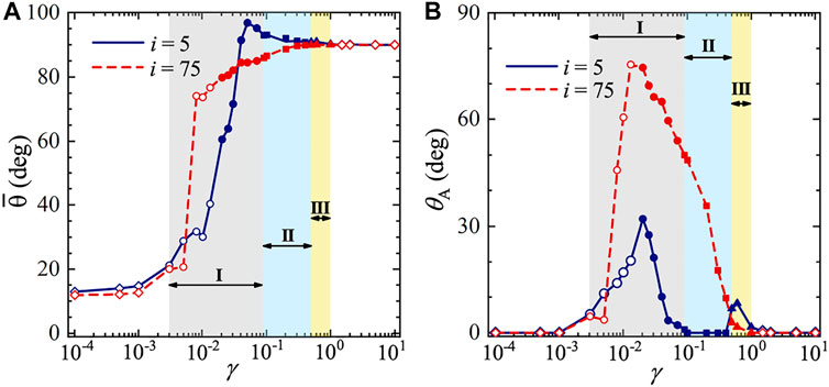
FIGURE 7. Mean inclination angle and amplitude of angular oscillation of the 5th and 75th plates as a function of dimensionless bending rigidity. (A) mean inclination angles, (B) amplitudes of angular oscillation. The fixed control parameters are the same as those in Figure 3. The diamonds, circles, squares and triangles represent the static reconfiguration mode, sectional waving mode (I), regular waving mode (II) and upright oscillation mode (III), respectively. The hollow and solid circles denote the sectional waving mode with quasi-periodic and periodic oscillations, respectively.

Beside the effect of bending rigidity, the effect of mass ratio on the dynamic behaviors of the array is also studied. Here the mass ratio β is allowed to vary in the range of 0.01–10, while the rest of the control parameters are kept unchanged (γ = 0.04, Re = 400 and d = 0.5). The variations of $\bar{\theta }$ and θ_A with β in the 5th and 75th plates are shown in Figure 8. From this figure, the regular waving mode and sectional waving mode can be identified in the ranges of 0.01 < β < 0.3 and 0.3 < β < 10, respectively. Thus, the transition from the regular waving mode to the sectional waving mode occurs when the mass ratio exceeds a threshold value of 0.3. From Figure 7, it is observed that such transition may also occur when the bending rigidity is below a threshold value. This implies that the increase of mass ratio and decrease of bending rigidity may influence the dynamics behavior similarly. An in-depth discussion on this issue will be provided in section 4.4.

FIGURE 8

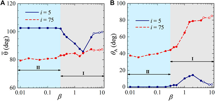
FIGURE 8. Mean inclination angles and amplitudes of angular oscillation of the 5th and 75th plates as a function of mass ratio. (A) Mean inclination angles, (B) amplitudes of angular oscillation. Fixed control parameters are: γ = 0.04, Re = 400, and d = 0.5. The squares, solid circles and hollow circles represent the regular waving mode, sectional waving mode with periodic oscillations, and sectional waving mode with quasi-periodic oscillations, respectively.

4.3 Influences of Gap Distance on the Dynamic Behaviors

For arrays with multiple wall-mounted flexible plates, the gap distance between adjacent plates also plays an important role in determining the dynamic behaviors. Here the dimensionless gap distance d is allowed to vary in the range of 0.1–1.0 (due to the limitation on size of the computational domain), and γ is allowed to vary in the range of 0.01–1.0. The fixed control parameters are: β = 1.0 and Re = 400. A map for the classification of dynamic modes in the two-dimensional parametric space of (γ, d) is shown in Figure 9. In this figure, five distinct modes, namely, static reconfiguration, sectional waving, regular waving, upright oscillation and cavity oscillation, can be identified.

FIGURE 9

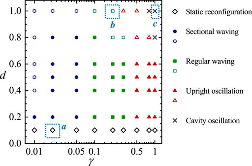
FIGURE 9. A map for the classification of dynamic modes in the space of (γ, d). The diamonds, circles, squares, triangles, and crosses denote the static reconfiguration mode, sectional waving mode, regular waving mode, upright oscillation mode, and cavity oscillation mode, respectively. The solid and hollow symbols represent periodic and quasi-periodic oscillations, respectively. The symbols in boxes represent the selected cases for which the wake structures will be displayed in Figure 10.

At a small gap distance (d = 0.1), the static reconfiguration is exhibited. At intermediate gap distances (0.2 ≤ d ≤ 0.6), the dynamic mode transits from sectional waving to regular waving and then to upright oscillation, with the increase of bending rigidity. This trend has already been revealed in section 4.2. At large gap distances (d = 0.8 and d = 1.0), with increasing bending rigidity, four dynamic modes, namely, sectional waving, regular waving, upright oscillation and cavity oscillation emerge in turn.

The patterns of motion in the plates and wake structures for some selected cases of Figure 9 are shown in Figure 10. One case of the static configuration mode is displayed in Figure 10A. The array has a high packing density and the plates behave like a single unit when interacting with the flow. The static deformations of the downstream plates are smaller than those in the front due to the shielding effect. This is in consistent with the results reported in Wang et al. [11]. A shear layer is stably attached on the top of the array. The instability of the shear layer can only be seen in the far wake downstream.

FIGURE 10

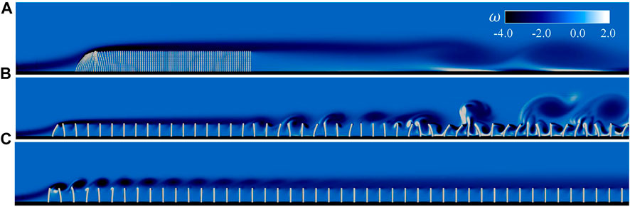
FIGURE 10. The patterns of motion and wake structures for some selected cases in Figure 9. (A) γ = 0.02, d = 0.1 (static reconfiguration mode), (B) γ = 0.2, d = 1.0 (regular waving mode with quasi-periodic oscillations), (C) γ = 1.0, d = 1.0 (cavity oscillation mode). Only the first 50 plates are displayed in (B) and (C).

One case of the regular waving mode is displayed in Figure 10B. Please note that the wake structure in the rear portion of the array (i > 30) become more complicated in comparison with the one displayed in Figure 3D. Some differences between the two cases are also exhibited in the oscillations of plates in the rear portion. Figure 11 shows the time series of the instantaneous inclination angle of the 75th plate, together with the normalized power spectrum and the contours of inclination angle in the space of index and time. From Figure 11, quasi-periodicity is clearly seen in the oscillation of the 75th plate. The complexity in the oscillations of the rear portion is introduced by the coexistent of Kelvin-Helmholtz (K-H) instability and instability associated with open-cavity flow. The latter type of instability only sets in when the gap distance becomes relatively large.

FIGURE 11

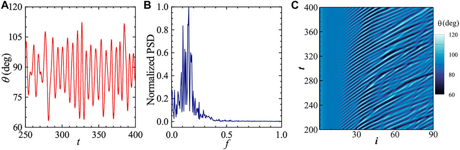
FIGURE 11. (A) Time history of inclination angle, (B) normalized power spectrum of angular oscillation, and (C) contours of inclination angle in space of plate index and time, for the 75th plate in the regular waving mode corresponding to Figure 10B.

One case of the cavity oscillation mode is displayed in Figure 10C. This dynamic mode only appears in sparsely packed arrays and is not observed in arrays with relatively small gap distance (such as the ones discussed in section 4.2). The mean inclination angles of the plates in the cavity oscillation mode are close to 90°, which is similar to those in the upright oscillation mode. However, some marked differences between these two dynamic modes are also observed. First, it is seen that in the cavity oscillation mode, the length scales of the vortices are close to d (Figure 10C), whereas the length scales of the vortices are much larger than d in the upright oscillation mode (Figure 3E). Second, the distributions of oscillating amplitudes along the array are also very different in the two modes (Figure 12). From Figure 12, it is seen that the cavity oscillation mode has a much narrower spread of index for the oscillating plates, in comparison with the upright oscillation mode. Moreover, the peak oscillating amplitude in the cavity oscillation mode is also much larger. For the cavity oscillation mode, a peak amplitude of 19° is achieved in the 3rd plate, whereas for the upright oscillation mode, the peak amplitude of 9° is achieved in the 18th plate.

FIGURE 12

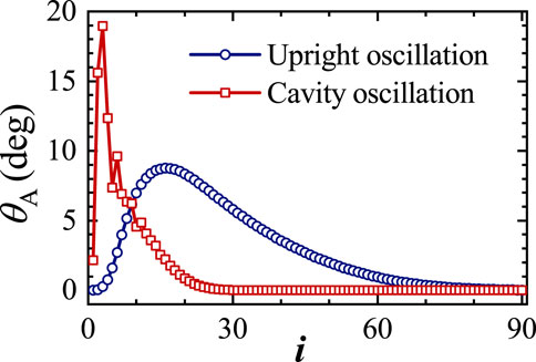
FIGURE 12. Distributions of oscillating amplitudes along the array for the upright oscillation mode and the cavity oscillation mode. The case of upright oscillation mode corresponds the one shown in Figure 3E, and the case of cavity oscillation mode corresponds the one shown in Figure 10C.

4.4 Frequency Selection Mechanisms of Different Dynamic Modes

In this section, the underlying physical mechanisms of each dynamic mode are discussed. In the study of flow-induced oscillations in single- and dual-plate systems, the oscillating frequencies were found to be locked onto the first or second natural frequency [10]. First, we examine whether this frequency selection phenomenon also exists in arrays composed of large numbers of flexible plates.

The natural frequencies of the flexible plates in the present study are estimated by those for a cantilever Euler-Bernoulli beam [10]. The dimensionless i-th order natural frequency of the cantilever Euler-Bernoulli beam is given by

$f_{ni}^{*}=\frac{{\tilde{f}}_{ni}^{*}L}{U_{\infty }}=\frac{k_i^2}{2\pi }\sqrt{\frac{\gamma }{\beta }},\mathrm{w}\mathrm{i}\mathrm{t}\mathrm{h}\cos k_i\cosh k_i+1=0.(8)$

Here ${\tilde{f}}_{ni}^{*}$ represents the dimensional natural frequency of the i-th order. The coefficients k_i for the first and second natural frequencies are: k₁ = 1.875 and k₂ = 4.694. When the cantilever beam is immersed in the fluid, the natural frequencies are modulated by the effect of added mass. The modulated i-th order (dimensionless) natural frequency is given by

$f_{ni}=\frac{k_i^2}{2\pi }\sqrt{\frac{\gamma }{\beta +C_m\cdot \pi /4}},(9)$

where the added mass coefficient C_m is set to 1.0 according to the empirical expression provided by Luhar et al. [32]. In addition, the natural frequencies of flexible plates immersed in the fluid can also be modulated by other effects [10], such as damping due to drag, prestress due to static deformation [33], and nonlinear effect due to large-amplitude oscillation. Since the influences of these nonlinear effects on natural frequencies are hard to quantify, f_ni is still used in the present work.

The 5th and 75th plates are regarded as representatives for the oscillations of the front and rear portions. The dominant frequencies of the two plates are plotted as a function of dimensionless bending rigidity and mass ratio in Figure 13A and Figure 13B, respectively. The first and second natural frequencies as a function of bending rigidity and mass ratio are also plotted in the figures for comparison. It is seen that the oscillating frequencies of the plates are always locked onto the first- or second-order natural frequency in all dynamics modes. For the sectional waving mode (regime I), the plates of the front portion oscillate at the second-order natural frequency, while the ones of the rear portion oscillate at the first-order natural frequency. For the regular waving mode (regime II), the plates of the rear portion oscillate at the first-order natural frequency (plates of the front portion remain stationary). For the upright oscillation mode (regime III), all plates oscillate at the first-order natural frequency. The superimposed shapes of the 5th and 75th plates throughout one oscillation cycle for different dynamic modes are shown in Figure 14. The orders of oscillation mode demonstrated in these shapes provides an additional evidence for the existence of frequency lock-in phenomenon. From Figure 13, it is also seen that increasing bending rigidity may influence the dynamics behaviors similarly as decreasing mass ratio (in terms of the transition from regime I to regime II). This can be explained by the fact that both the increase of bending rigidity or the decrease of mass ratio will result in higher natural frequencies of the plates.

FIGURE 13

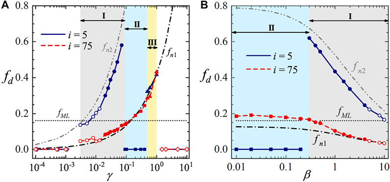
FIGURE 13. Dominant oscillating frequencies of the 5th and the 75th plates as a function of (A) dimensionless bending rigidity, and (B) mass ratio. The fixed control parameters are: Re = 400, d = 0.5, β = 1.0 for (A), and Re = 400, d = 0.5, γ = 0.04 for (B). The diamonds, circles, squares and triangles represent the static reconfiguration, sectional waving, regular waving and upright oscillation mode, respectively. The hollow and solid circles denote the sectional waving modes with quasi-periodic and periodic oscillations, respectively. The first and second natural frequencies are represented by a dash-dotted line and a dash-double-dotted line, respectively. The estimated frequency of mixing layer instability is represented by a horizontal dotted line.

FIGURE 14

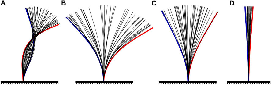
FIGURE 14. The superimposed shapes of the 5th or the 75th plates throughout one oscillation cycle in different dynamic modes. (A) 5th plate of the sectional waving mode (γ = 0.02), (B) 75th plate of the sectional waving mode (γ = 0.02), (C) 75th plate of the regular waving mode (γ = 0.2). (D) 75th plate of the upright oscillation mode (γ = 0.5).

Next, a discussion on the flow instabilities which drive the oscillations of the plates is provided. Basically, three types of flow instabilities, namely, Kelvin-Helmholtz (K-H) instability, shear-layer related vortex shedding, and instability in open-cavity flow, are involved in the system studied here. The FSI mechanisms associated with them will be addressed separately as follows.

In some previous works on vegetative flows, the K-H instability of mixing layer was considered to be the dominant mechanism for generating the coherent waving motions [15, 16]. In this study, it is also observed that the coherent waving motions in the sectional waving and regular waving modes are always accompanied by large-scale vortices developed on top of the array behind a stable or nearly stable mixing (shear) layer. The K-H instability is a classic problem in fluid mechanics. The frequency of K-H instability can be estimated using the following empirical expression [15]:

$f_{ML}=S{t}_n\left(\frac{U_1+U_2}{2\mathrm{\Theta }}\right),(10)$

where St_n and Θ denote the natural Strouhal number and the momentum thickness of the mixing layer, respectively. U₁ and U₂ represent the low-stream and high-stream velocities associated with the mixing layer, respectively [22]. In the configuration of the present work, we take U₁ = 0 and U₂ = U_∞. Based on experimental data available, the value of St_n ≈ 0.032 is considered to yield satisfactory results in predictions [34]. The momentum thickness Θ can be estimated by [22].

$\mathrm{\Theta }={\int }_{-\infty }^{\infty }\left\{\frac{1}{4}-{\left[\frac{U\left(y\right)-\frac{1}{2}\left(U_1+U_2\right)}{U_2-U_1}\right]}^2\right\}dy,(11)$

where U (y) denotes the averaged streamwise velocity profile. In the present work, the averaged velocity profile of flow past an array with rigid plates (taking flexible plates with extremely high rigidity as an approximation) is used to estimate the frequency of mixing layer instability. The velocity profile at i = 30 is chosen here since the stable shear layer is fully developed at this position and the influence of entrance effect becomes negligible at this position (the location is denoted by a dashed line in Figure 3F). The frequency of K-H instability estimated by using Eq. 10 is approximately 0.16, which is close to the prediction made by O’Conner et al. [22]. Since the plates within the range of mixing-layer development stay almost upright in the regular waving mode, the effect of plate deformation on the averaged velocity profile is negligible. Thus, this estimated frequency is a good approximate for an array composed of plates with moderate bending rigidities.

From Figure 13, it is seen that in the regular waving mode, oscillating frequency of the rear plate is very close to the estimated frequency of K-H instability. This finding suggests that the development of coherent waving motion at the rear portion is governed by a coupled mechanism of elastic property of the structure and instability of the mixing layer. In the sectional wave mode, the oscillating frequency of the rear plate is lower than the estimated frequency of K-H instability. The discrepancy in frequency can be explained by the fact that a long stable mixing layer has not been fully developed on the top of the array (see Figure 3B and Figure 3C).

The oscillations in the front portion of the sectional waving mode and oscillations in the upright oscillation mode are driven by another type of shear layer instability related to vortex-shedding excitation. Although such excitation source shares some similarities with the K-H instability aforementioned. The difference between them is also evident. Here the vortex shedding is triggered by the pinch-off of a very short shear layer (see Figure 3B, Figure 3C and Figure 3E). As a result, the dimensionless frequency (Strouhal number) of vortex shedding cannot can be predicted by using the empirical formula for K-H instability (i.e., Eq. (10)). This vortex-shedding phenomenon also resembles that observed in flows over a bluff body [35] (such as a thin vertical plate or a flat-top rectangle). However, the two types of vortex shedding phenomena differ in two aspects. First, two shear layers are involved in flows over a bluff body, while only one shear layer is involved here. Second, the presence of multiple plates near the shear layer in the current study creates a boundary with more complex geometry. Due to the existence of marked differences, the dimensionless frequencies (Strouhal numbers) in some cases of these two dynamics modes may deviate significantly from those of the vortex shedding over commonly seen bluff bodies (such as circular and square cylinders).

The oscillation in the cavity oscillation mode is driven by instability associated with the open-cavity flow. The open-cavity flow is another classic problem in fluid mechanics. The dimensionless oscillating frequency in open-cavity flows can be estimated empirically by using the Rossiter’s formula [10, 36]:

$f_c=\frac{n-\alpha }{1/\kappa +M}\cdot \frac{1}{d},(12)$

where M is the Mach number (M = 0 for incompressible flow). n is the order of Rossiter mode (n = 1, 2, … ) and only n = 1 is considered in the present study. To fit the experimental data on open-cavity flows, the empirical constants κ and α are set to 0.57 and 0.25 [36], respectively.

In the cavity oscillation mode, the oscillating frequency of the plates is also found to be locked onto the first natural frequency. For the case shown in Figure 10C, the first natural frequency of the plates is around 0.419, while the estimated oscillating frequency of open-cavity flow is 0.428. Theoretically, as the gap distance increases further, high-order Rossiter modes may also emerge in a specific parameter range, when the frequencies of high-order Rossiter modes are close to the first natural frequency. The high-order modes are never observed in the present study due to the limited parameter range considered here.

5 Conclusion

In this paper, the interactions of a large array of wall-mounted flexible plates with an oncoming laminar boundary-layer flow are investigated systematically by numerical simulations. The influences of some control parameters, such as bending rigidity, mass ratio and gap distance (between adjacent plates), on the dynamic behaviors of the arrays are explored. With the variation of control parameters, five distinct modes, namely, static reconfiguration, sectional waving, regular waving, upright oscillation and cavity oscillation are identified. The pattern of motion in the plates and wake structure for each dynamic mode are demonstrated.

The frequency lock-in and underlying physical mechanism associated with different dynamics modes are elucidated. It is found that the frequency selection is governed by a coupling mechanism of elastic property and flow instability. In the sectional waving mode, the oscillating frequency in the front portion of the array is locked onto the second-order natural frequency. In other dynamics modes, the oscillating frequency of the plates is always locked onto the first-order natural frequency. Three types of flow instabilities that drive the oscillations of the plates are identified. The K-H instability is found to be the excitation source for the rear portion of the array in the sectional waving mode and regular waving mode. In the upright oscillation mode and front portion of the sectional waving mode, the shear layer instability related to vortex shedding is found to be the excitation source. The instability associated with open-cavity flow is found to be the excitation source in the cavity oscillation mode.

There are several avenues for further research. First, the dynamic interactions of wall-mounted flexible plates in an oscillatory flow should be investigated to evaluate the universality of the frequency lock-in mechanism addressed here. Second, how the motion of the plates and flow structure are affected by gravity and buoyancy needs further study. Third, drag reduction and energy absorption associated with different dynamic modes warrant further investigation. Last, three-dimensional simulations should be conducted to explore the 3D effects (such as reduced blockage and lateral flow) on the dynamic interactions among flexible structures.

Data Availability Statement

The raw data supporting the conclusion of this article will be made available by the authors, without undue reservation.

Author Contributions

XiaZ: designed the study, conducted the numerical simulations, performed the data analyses and visualization, wrote the manuscript. YL: analysed the data and assisted in visualization. XinZ: interpreted results and revised the manuscript.

Funding

This work was supported by the China Postdoctoral Science Foundation under grant number 2021M690466, the National Natural Science Foundation of China under Grant Nos 11372331, 11772338, 12172361.

Conflict of Interest

The authors declare that the research was conducted in the absence of any commercial or financial relationships that could be construed as a potential conflict of interest.

Publisher’s Note

All claims expressed in this article are solely those of the authors and do not necessarily represent those of their affiliated organizations, or those of the publisher, the editors and the reviewers. Any product that may be evaluated in this article, or claim that may be made by its manufacturer, is not guaranteed or endorsed by the publisher.

References

1. Luhar M, Nepf HM. Flow-induced Reconfiguration of Buoyant and Flexible Aquatic Vegetation. Limnol Oceanogr (2011) 56:2003–17. doi:10.4319/lo.2011.56.6.2003

CrossRef Full Text | Google Scholar

2. Leclercq T, Peake N, de Langre E. Does Flutter Prevent Drag Reduction by Reconfiguration? Proc R Soc A (2018) 474:20170678. doi:10.1098/rspa.2017.0678

PubMed Abstract | CrossRef Full Text | Google Scholar

3. Leclercq T, de Langre E. Reconfiguration of Elastic Blades in Oscillatory Flow. J Fluid Mech (2018) 838:606–30. doi:10.1017/jfm.2017.910

CrossRef Full Text | Google Scholar

4. Henriquez S, Barrero-Gil A. Reconfiguration of Flexible Plates in Sheared Flow. Mech Res Commun (2014) 62:1–4. doi:10.1016/j.mechrescom.2014.08.001

CrossRef Full Text | Google Scholar

5. Leclercq T, de Langre E. Drag Reduction by Elastic Reconfiguration of Non-uniform Beams in Non-uniform Flows. J Fluids Structures (2016) 60:114–29. doi:10.1016/j.jfluidstructs.2015.10.007

CrossRef Full Text | Google Scholar

6. Jin YQ, Kim JT, Chamorro LP. Instability-driven Frequency Decoupling between Structure Dynamics and Wake Fluctuations. Phys Rev Fluids (2018) 3:044701. doi:10.1103/physrevfluids.3.044701

CrossRef Full Text | Google Scholar

7. Jin Y, Kim J-T, Hong L, Chamorro LP. Flow-induced Oscillations of Low-Aspect-Ratio Flexible Plates with Various Tip Geometries. Phys Fluids (2018) 30:097102. doi:10.1063/1.5046950

CrossRef Full Text | Google Scholar

8. Jin Y, Kim J-T, Fu S, Chamorro LP. Flow-induced Motions of Flexible Plates: Fluttering, Twisting and Orbital Modes. J Fluid Mech (2019) 864:273–85. doi:10.1017/jfm.2019.40

CrossRef Full Text | Google Scholar

9. Jin Y, Kim J-T, Mao Z, Chamorro LP. On the Couple Dynamics of wall-mounted Flexible Plates in Tandem. J Fluid Mech (2018) 852:R2. doi:10.1017/jfm.2018.580

CrossRef Full Text | Google Scholar

10. Zhang X, He G, Zhang X. Fluid-structure Interactions of Single and Dual wall-mounted 2D Flexible Filaments in a Laminar Boundary Layer. J Fluids Structures (2020) 92:102787. doi:10.1016/j.jfluidstructs.2019.102787

CrossRef Full Text | Google Scholar

11. Wang S, Ryu JH, Yang JM, Chen YJ, He GQ, Sung HJ. Vertically Clamped Flexible Flags in a Poiseuille Flow. Phys Fluids (2020) 32:031902. doi:10.1063/1.5142567

CrossRef Full Text | Google Scholar

12. Chen Y, Ryu J, Liu Y, Sung HJ. Flapping Dynamics of Vertically Clamped Three-Dimensional Flexible Flags in a Poiseuille Flow. Phys Fluids (2020) 32:071905. doi:10.1063/5.0010835

CrossRef Full Text | Google Scholar

13. de Langre E. Effects of Wind on Plants. Annu Rev Fluid Mech (2008) 40:141–68. doi:10.1146/annurev.fluid.40.111406.102135

CrossRef Full Text | Google Scholar

14. Nepf HM. Flow and Transport in Regions with Aquatic Vegetation. Annu Rev Fluid Mech (2012) 44:123–42. doi:10.1146/annurev-fluid-120710-101048

CrossRef Full Text | Google Scholar

15. Ghisalberti M, Nepf HM. Mixing Layers and Coherent Structures in Vegetated Aquatic Flows. J Geophys Res Oceans (2002) 107:3–1. doi:10.1029/2001jc000871

CrossRef Full Text | Google Scholar

16. Ghisalberti M, Nepf HM. The Limited Growth of Vegetated Shear Layers. Water Resour Res (2004) 40:W07502. doi:10.1029/2003WR002776

CrossRef Full Text | Google Scholar

17. Dupont S, Gosselin F, Py C, de Langre E, Hemon P, Brunet Y. Modelling Waving Crops Using Large-Eddy Simulation: Comparison with Experiments and a Linear Stability Analysis. J Fluid Mech (2010) 652:5–44. doi:10.1017/s0022112010000686

CrossRef Full Text | Google Scholar

18. Py C, de Langre E, Moulia B. The Mixing Layer Instability of Wind over a Flexible Crop Canopy. Comptes Rendus Mécanique (2004) 332:613–8. doi:10.1016/j.crme.2004.03.005

CrossRef Full Text | Google Scholar

19. Py C, de Langre E, Moulia B, Hémon P. Measurement of Wind-Induced Motion of Crop Canopies from Digital Video Images. Agric For Meteorology (2005) 130:223–36. doi:10.1016/j.agrformet.2005.03.008

CrossRef Full Text | Google Scholar

20. Py C, de Langre E, Moulia B. A Frequency Lock-In Mechanism in the Interaction between Wind and Crop Canopies. J Fluid Mech (2006) 568:425–49. doi:10.1017/s0022112006002667

CrossRef Full Text | Google Scholar

21. Wong CY, Trinh PH, Chapman SJ. Shear-induced Instabilities of Flows through Submerged Vegetation. J Fluid Mech (2020) 891. doi:10.1017/jfm.2020.151

CrossRef Full Text | Google Scholar

22. O’Connor J, Revell A. Dynamic Interactions of Multiple wall-mounted Flexible Flaps. J Fluid Mech (2019) 870:189–216. doi:10.1017/jfm.2019.266

CrossRef Full Text | Google Scholar

23. Fang Z, Gong C, Revell A, O’Connor J. Fluid-structure Interaction of a Vegetation Canopy in the Mixing Layer. J Fluids Structures (2022) 109:103467. doi:10.1016/j.jfluidstructs.2021.103467

CrossRef Full Text | Google Scholar

24. Huang W-X, Shin SJ, Sung HJ. Simulation of Flexible Filaments in a Uniform Flow by the Immersed Boundary Method. J Comput Phys (2007) 226:2206–28. doi:10.1016/j.jcp.2007.07.002

CrossRef Full Text | Google Scholar

25. Roma AM, Peskin CS, Berger MJ. An Adaptive Version of the Immersed Boundary Method. J Comput Phys (1999) 153:509–34. doi:10.1006/jcph.1999.6293

CrossRef Full Text | Google Scholar

26. Wang S, Zhang X. An Immersed Boundary Method Based on Discrete Stream Function Formulation for Two- and Three-Dimensional Incompressible Flows. J Comput Phys (2011) 230:3479–99. doi:10.1016/j.jcp.2011.01.045

CrossRef Full Text | Google Scholar

27. Colonius T, Taira K. A Fast Immersed Boundary Method Using a Nullspace Approach and Multi-Domain Far-Field Boundary Conditions. Comput Methods Appl Mech Eng (2008) 197:2131–46. doi:10.1016/j.cma.2007.08.014

CrossRef Full Text | Google Scholar

28. Chang W, Giraldo F, Perot B. Analysis of an Exact Fractional Step Method. J Comput Phys (2002) 180:183–99. doi:10.1006/jcph.2002.7087

CrossRef Full Text | Google Scholar

29. Wang S, He G, Zhang X. Parallel Computing Strategy for a Flow Solver Based on Immersed Boundary Method and Discrete Stream-Function Formulation. Comput Fluids (2013) 88:210–24. doi:10.1016/j.compfluid.2013.09.001

CrossRef Full Text | Google Scholar

30. Zhu X, He G, Zhang X. Numerical Study on Hydrodynamic Effect of Flexibility in a Self-Propelled Plunging Foil. Comput Fluids (2014) 97:1–20. doi:10.1016/j.compfluid.2014.03.031

CrossRef Full Text | Google Scholar

31. Dai L, He G, Zhang X. Self-propelled Swimming of a Flexible Plunging Foil Near a Solid wall. Bioinspir Biomim (2016) 11:046005. doi:10.1088/1748-3190/11/4/046005

PubMed Abstract | CrossRef Full Text | Google Scholar

32. Luhar M, Nepf HM. Wave-induced Dynamics of Flexible Blades. J Fluids Structures (2016) 61:20–41. doi:10.1016/j.jfluidstructs.2015.11.007

CrossRef Full Text | Google Scholar

33. Heylen W, Lammens S, Sas P. Modal Analysis Theory and Testing, 200. Leuven, Belgium: Katholieke Universiteit Leuven (1997).

Google Scholar

34. Ho C, Huerre P. Perturbed Free Shear Layers. Annu Rev Fluid Mech (1984) 16:365–422. doi:10.1146/annurev.fl.16.010184.002053

CrossRef Full Text | Google Scholar

35. Matshumoto M. Vortex Shedding of bluff Bodies: a Review. J Fluids Structures (1999) 13:791–811.

Google Scholar

36. Gloerfelt X. Cavity Noise. In: VKI Lectures: Aeroacoustics of Wall-Bounded Flow. Von Kármán Institute (2009). p. 15–16.

Google Scholar