Advection–Diffusion Lattice Boltzmann Method With and Without Dynamical Filter

In multi-component flow and/or thermal flows, when the diffusion coefficient of the advection–diffusion equation is relatively small, the relaxation coefficient in the lattice Boltzmann method will be close to 0.5, which will lead to numerical instability. The stability conditions will become more severe, when there are high gradient regions in the computational domain. In order to improve the stability of advection–diffusion lattice Boltzmann method to simulate scalar transport in complex flow, a hybrid regularized collision operators and a dynamic filtering method which is suitable for the convection-diffusion lattice Boltzmann method are proposed in this paper. The advection–diffusion lattice Boltzmann method is first tested in uniform flow with smooth and discontinuous initial conditions. Then the scalar transport in doubly periodic shear layer flow is tested, which is sensitive to numerical stability. The adaptive dynamic filtering method is also tested. The results are compared to the classical finite difference method and to the lattice Boltzmann method using the projection-based regularized and standard Bahtnagar-Gross-Krook collision operator. The results show that the hybrid regularized collision operator has advantages in simulating the scalar advection-diffusion problem with small diffusion coefficient. In addition, the adaptive filtering method can also improve the numerical stability of the lattice Boltzmann method with limited numerical dissipation.

1 Introduction

Species transport and heat transfer flows are widely present in real-world systems with complicated geometry (gas turbines, burners, furnaces, and so on), and accurate numerical simulation of these processes is key to initial design. The governing equations consist of three main components: (a) Navier–Stokes equations for the fluid, (b) heat transport equation and (c) a set of transport equations for the species. Conventional numerical methods for solving these equations include finite difference methods, finite volume methods, and finite element methods. Although initially developed to solve the Navier–Stokes (NS) equation, lattice Boltzmann method have been extended to a variety of applications and flows [1–3]. The local nature of the time evolution of the LBM helps to simplify the numerical coding process, improve the parallel scalability of the algorithm, and make the implementation of the complex boundary conditions straightforward. The disadvantage of LBM is that as the number of lattice velocity sets increases, more memory storage will be required. Despite the latter issue, the lattice Boltzmann method has emerged as a potential alternative for simulating a range of complex flows throughout the last decade.

The advection-diffusion or passive scalar LBM is widely used in the literature, especially under the assumption of incompressible flow [4–6]. In this approach, the LBM flow solver is used to model the conservation of mass and momentum, while the temperature and species fields were handled using other sets of distribution functions. And it is assumed that the species and temperature distribution have little effect on the density, so the effect of species and temperature changes on the flow can be reflected by adding body force terms in the LBM flow solver. Hosseini [7, 8] modified the classical advection-diffusion LBM, which can consider the effects of the changes of thermophysical parameters and transport coefficients, and used the modified LBM to simulate the reacting flows with detailed thermo-chemical models.

However, when the relaxation factor in LBM is very close to 0.5, it is easy to cause instability. The origin of LBM instability has been actively studied and remains an open topic [9, 10]. An extension of the von Neumann linear analysis showed that modal interactions due to the error in the time and space discretization can lead to severe linear instabilities [11]. A linear perturbative analysis methodology has been proposed to study the stability properties of the isothermal discrete velocity Boltzmann equations using the Knudsen number as parameter [12]. Linear stability analysis of isothermal lattice Boltzmann methods has been carried out to investigate the impact of the collision model on numerical stability [13–16]. The modal couplings depending on the exact value of the relaxation time, mean flow quantities, or even mesh resolution can appear and make a perfectly stable wave become unstable. For the compressible thermal flow, a spectral study of the compressible hybrid lattice Boltzmann method on standard lattice has been proposed to study the effect of the choice of numerical parameters on computational stability [17]. Suga [18] performed a linear stability analysis of the two-dimensional LBM for advection-diffusion equation and derived stable regions for different dimensionless relaxation coefficients. Hosseini [19] used the von Neumann method to analyze the stability of the LBM for advection-diffusion equation, and investigated the effects of different distribution functions and different parameters such as lattice sound velocity on the stability region. The main consequence of the LBM instability is to create numerical oscillations during the simulation, which are mainly characterized by high-frequency waves propagating throughout the computational domain. The numerical instability become more severe when discontinuous initial conditions, inappropriate boundary conditions, or high gradient regions exist in the computational domain. In order to expand the stability region of LBM, various theoretical methods have been proposed, including: multiple relaxation times [20], regularization techniques [21], entropic models [22].

Compared with the method of theoretically modifying the LBM, other studies use filtering methods to improve the stability of the calculation. The filtering methodology has already been extensively discussed for fluid flow simulations based on LBM, including static [23, 24] and adaptive filtering strategies [25, 26]. Ricot [23] proposed a high-order spatial filter to stabilize the LBM by increasing the dissipation in the high wavenumber range where the instabilities occur. However, the use of high-order filters will increase the stencil of LBM and reduce computational efficiency. Marié [26] et al. proposed a dynamical adaptive filtering method to improve stability of LBM. In this method, the filter coefficients depend on the local shear stress, which can improve the computational stability without introducing excessive numerical dissipation. Moreover, the dynamical filtering strategy can work with low-order stencil, which is consistent with the LBM.

In this paper, the advection–diffusion lattice Boltzmann method is first tested in uniform flow with smooth and discontinuous initial conditions. In order to test the ability of advection-diffusion LBM in simulating scalar transport problems in complex flow, we use the scalar transport in doubly periodic shear layer flow as an example to compare the results of advection-diffusion LBM using different collision operators respectively. These collision operators are the projection based regularized collision operator, classical BGK collision operator and the hybrid regularized collision operator. Further, the effect of using dynamic filtering method to improve the stability of advection-diffusion LBM is explored. In this filtering method, the gradient of the transport scalar is selected as the sensitive variable. In the region with smooth variable distribution, the intensity coefficient of the filter is small to avoid introducing too much artificial dissipation, while in the region with large gradient distribution or discontinuity, the intensity coefficient of the filter is large to suppress the development of numerical oscillation.

The rest of the paper is organized as follows. A brief presentation of the LBM is given in Section 2. The filtering strategy is described in Section 3. The results of the scalar transport in uniform flow and doubly periodic shear layer flow obtained with the numerical method are presented in Section 4. Finally, a brief conclusion is given.

2 Lattice Boltzmann Model

In the context of the present study a weakly compressible 2-D recursive regularization lattice model has been used as the flow field solver. The same grid structure and spacing is used for passive scalar fields.

2.1 LBM for the Flow Field

With the initial solution simply defined by initial macroscopic fields $\rho \left(x,t\right), u_{\alpha }\left(x,t\right)$ , with $\dot{m}$ the mass source and $F_a$ the volume force term, the step-by-step lattice Boltzmann method that predicts $\rho \left(x,t+\Delta t\right), u_{\alpha }\left(x,t+\Delta t\right)$ following an approximate Navier-Stokes system is given.

Step 1. : Equilibrium constructionConsidering the fourth order Hermite expansion of Maxwell-Boltzmann distribution, one can obtain the equilibrium distribution function [27].

$f_i^{eq}={\omega }_i\left\{H^{\left(0\right)}\rho +\frac{H_{\text{i}\alpha }^{\left(1\right)}}{c_s^2}\rho u_{\alpha }+\frac{H_{\text{i}\alpha \beta }^{\left(2\right)}}{2c_s^4}\left[\rho u_{\alpha }{u}_{\beta }\right]+\frac{H_{\text{i}\alpha \beta \gamma }^{\left(3\right)}}{6c_s^6}\left[\rho u_a{u}_{\beta }{u}_{\gamma }\right]+\frac{H_{\text{i}\alpha \beta \gamma \delta }^{\left(4\right)}}{24c_s^8}\left[\rho u_a{u}_{\beta }{u}_{\gamma }{u}_{\delta }\right]\right\}(1)$

where $w_i$ is the weight coefficient, and $c_s=1/\sqrt{3}$ is the speed of sound in lattice units. The discrete velocity vectors and weight coefficients are defined as

$c_i=\left(\begin{array}{c}0 1 0 -1 0 1 -1 -1 1\\ 0 0 1 0 -1 1 1 -1 -1\end{array}\right)(2)$

$w_0=4/9,w_{i=1\sim 4}=1/9,w_{i=5\sim 8}=1/36(3)$

The Hermite polynomials read

$H_i^{\left(0\right)}=1,H_{i\alpha }^{\left(1\right)}=c_{i\alpha }\mathrm{，}{H}_{i\alpha \beta }^{\left(2\right)}=c_{i\alpha }{c}_{i\beta }-c_s^2{\delta }_{\alpha \beta }(\mathrm{4a})$

$H_{i\alpha \beta \gamma }^{\left(3\right)}=c_{i\alpha }{c}_{i\beta }{c}_{i\gamma }-c_s^2\left[c_{i\alpha }{\delta }_{\beta \gamma }+c_{i\beta }{\delta }_{\gamma \alpha }+c_{i\gamma }{\delta }_{\alpha \beta }\right](\mathrm{4b})$

$H_{i\alpha \beta \gamma \delta }^{\left(4\right)}=c_{i\alpha }{c}_{i\beta }{c}_{i\gamma }{c}_{i\delta }-c_s^2\left[c_{i\alpha }{c}_{i\beta }{\delta }_{\gamma \delta }+c_{i\alpha }{c}_{i\gamma }{\delta }_{\beta \delta }+c_{i\alpha }{c}_{i\delta }{\delta }_{\beta \gamma } +c_{i\beta }{c}_{i\gamma }{\delta }_{\alpha \delta }+c_{i\beta }{c}_{i\delta }{\delta }_{\alpha \gamma }+c_{i\gamma }{c}_{i\delta }{\delta }_{\alpha \beta }\right]+c_s^4\left[{\delta }_{\alpha \beta }{\delta }_{\gamma \delta }+{\delta }_{\alpha \gamma }{\delta }_{\beta \delta }+{\delta }_{\alpha \delta }{\delta }_{\beta \gamma }\right](\mathrm{4c})$

The third-order Hermite polynomials supported by the D2Q9 basis are $H_{\text{i}xxy}^{\left(3\right)}$ and $H_{\text{i}yyx}^{\left(3\right)}$, and the fourth-order Hermite polynomials supported by the D2Q9 basis is $H_{\text{i}xxyy}^{\left(4\right)}$.

Step 2. : Force constructionThe forcing population is extended to second order [28, 29],

$F_i={\omega }_i\left\{H^{\left(0\right)}{a}^{F,\left(0\right)}+\frac{H_{\text{i}\alpha }^{\left(1\right)}}{c_s^2}{a}_{\alpha }^{F,\left(1\right)}+\frac{H_{\text{i}\alpha \beta }^{\left(2\right)}}{2c_s^4}{a}_{\alpha \beta }^{F,\left(2\right)}\right\}(5)$

with its Hermite moments defined as

$a_{\alpha \beta }^F=-\frac{\partial D_{\alpha \beta \gamma }^{f^{eq,\left(3\right)}}}{\partial x_{\gamma }}+\rho c_s^2\frac{2}{3}\frac{\partial u_{\gamma }}{\partial x_{\gamma }}{\delta }_{\alpha \beta }+\rho F_a{u}_{\beta }+\rho u_a{F}_{\beta }-\dot{m}{u}_{\alpha }{u}_{\beta }(6)$

$a_{\alpha }^{F,\left(1\right)}=\rho F_a(7)$

$a^{F,\left(0\right)}=\dot{m}(8)$

with $D_{\alpha \beta \gamma }^{f^{eq,\left(3\right)}}$ the isotropy defect of the equilibrium distribution function. Here, for the D2Q9 lattice, the isotropy defects are $D_{xxx}^{f^{eq,\left(3\right)}}=\rho u_x^3$ and $D_{xxy}^{f^{eq,\left(3\right)}}=0$.

Step 3. : Non-equilibrium constructionUsing the BGK collision operator, the non-equilibrium distribution function is obtained as:

${\overline{f}}_i^{neq}={\overline{f}}_i-f_i^{eq}+\frac{\Delta t}{2}{F}_i(9)$

However, when the relaxation factor of the BGK form of the LBM model is close to the critical value, the accuracy will be reduced. The use of regularized collision operators can effectively broaden the application range of the LBM model. For simulating isothermal flow with standard D2Q9 model, the recursive regularization collision operator with the third-order Hermite expansion [30] can obtain stable result, the non-equilibrium distribution function is obtained as:

${\overline{f}}_i^{neq}={\omega }_i\left\{\frac{H_{\text{i}\alpha \beta }^{\left(2\right)}}{2c_S^4}{\Pi }_{\alpha \beta }^{{\overline{f}}^{neq},\left(2\right)}+\frac{H_{\text{i}\alpha \beta \gamma }^{\left(3\right)}}{6c_S^6} \left(u_{\alpha }{\Pi }_{\beta \gamma }^{{\overline{f}}^{neq},\left(2\right)}+u_{\beta }{\Pi }_{\gamma \alpha }^{{\overline{f}}^{neq},\left(2\right)}+u_{\gamma }{\Pi }_{\alpha \beta }^{{\overline{f}}^{neq},\left(2\right)}\right)\right\}(10)$

where the second order moment of the non-equilibrium distribution function is

${\Pi }_{\alpha \beta }^{{\overline{f}}^{neq},\left(2\right)} ={\displaystyle \sum }_i^q{c}_{i\alpha }{c}_{i\beta }\left({\overline{f}}_i-f_i^{eq}+\frac{\Delta t}{2}{F}_i\right)(11)$

Step 4. : Collision processWith the equilibrium distribution function $f_i^{eq}$ , forcing population $F_i$ and non-equilibrium distribution function ${\overline{f}}_i^{neq}$ are given in the previous steps, compute the collided distribution function as

$f_i^{col}\left(t,x\right)=f_i^{eq}\left(t,x\right)+\left(1-\frac{\Delta t}{\overline{\tau }}\right){\overline{f}}_i^{neq}\left(t,x\right)+\frac{\Delta t}{2}{F}_i\left(t,x\right)(12)$

It should be noted that the prefactor commonly used with Guo’s forcing methodology [28], i.e., (1 − ∆t/2τ), is modified to ∆t/2 because discrete effects are accounted for in the definition of the second-order non-equilibrium contribution (Eq. 11).The relationship between the relaxation time $\overline{\tau }$ and the viscosity $\nu$ is as follows:

$\nu = c_s^2\left(\overline{\tau }-\frac{\Delta t}{2}\right)(13)$

Step 5. : Streaming processTransport the distribution to neighbouring nodes according to

${\overline{f}}_i\left(t+\Delta t,x\right)=f_i^{col}\left(t,x-c_i\Delta t\right)(14)$

Step 6. : Update macroscopic variablesThe density $\rho$ and velocity $u$ are (weighted) sums of the distribution ${\overline{f}}_i$.

$\rho \left(t+\Delta t,x\right)={\displaystyle \sum }_i^q{\overline{f}}_i\left(t+\Delta t,x\right)+\frac{\Delta t}{2}\dot{m}\left(t+\Delta t,x\right)(15)$

$\rho u_{\alpha }\left(t+\Delta t,x\right)={\displaystyle \sum }_i^q{c}_{i\alpha }{\overline{f}}_i\left(t+\Delta t,x\right)+\frac{\Delta t}{2}\left[\rho F_{\alpha }\right]\left(t+\Delta t,x\right)(16)$

2.2 LBM for the Scalar Field

For a scalar field $C$, the governing equation of the convection-diffusion process is:

$\frac{\partial C}{\partial t}+\nabla \cdot \left(C\mathit{u}\right)=\nabla \cdot \left(D\nabla C\right)+F(17)$

where $C$ represents a conserved physical quantity, such as temperature or component concentration. The left side of the equation describes the convection process of the scalar $C$ along with the external fluid velocity $\mathbf{u }$. The first term on the right side of the equation is the diffusion term, where $D$ is the diffusion coefficient, and the second term $F$ is the source term.

The advection–diffusion LBM is based on the following space–time evolution equation for the distribution function:

$g_i\left(x+c_i\Delta t,t+\Delta t\right)-g_i\left(x,t\right)={\Omega }_i+\left(1-\frac{\Delta t}{2{\tau }_g}\right)F_i\left(x,t\right)(18)$

where the first item on the right-hand side is the collision source item. The prefactor (1 − ∆t/2τ_g) was proposed by Guo et al. to reduce discrete effect issues [28]. For the collision operator in the form of BGK:

${\Omega }_i\left(x,t\right)=-\frac{1}{{\tau }_g} \left(g_i\left(x,t\right)-g_i^{eq}\left(x,t\right)\right)(19)$

The second item on the right-hand side of Eq. 17 is the source term used to correct the error caused by the convection term [31]:

$F_i\left(x,t\right)=w_i\frac{{\mathit{c}}_{\mathit{i}}\cdot {\partial }_t\left(C\mathit{u}\right)}{c_s^2}(20)$

The time derivative is computed by first-order Euler method.

The relationship between the relaxation time ${\tau }_g$ and the diffusion coefficient $D$ is as follows:

$D=c_s^2\left({\tau }_g-\frac{\Delta t}{2}\right)(21)$

Given the reduced number of moments conserved in the advection–diffusion model and absence of non-linear velocity terms in the target macroscopic equation, the equilibrium distribution function can be truncated at first order

$g_{\dot{l}}^{eq}=w_{i}C\left(1+\frac{{\mathit{c}}_{\mathit{i}}\cdot \mathit{u}}{c_s^2}\right)(22)$

The D2Q9 model is also used to solve the scalar transport process in this paper, because it is more robust and accurate than the D2Q4 or D2Q5 model when the convection is strong. The specific values of its lattice parameters are shown in the previous section.

The advection–diffusion LBM algorithm is divided into two parts: collision process and streaming process.

The collision process is:

$g_{\dot{l}}^{col}\left(x,t\right)=g_{\dot{l}}^{eq}\left(x,t\right)+\left(1-\frac{\Delta t}{{\tau }_g}\right)g_{\dot{l}}^{neq}\left(x,t\right)+\left(1-\frac{\Delta t}{2{\tau }_g}\right)F_i\left(x,t\right)(23)$

Among them, $g_{\dot{l}}^{neq}$ is the off-equilibrium distribution, in the collision kernel of the BGK form, $g_{\dot{l}}^{neq}=g_i-g_i^{eq}$. For the regularized collision operator, the off-equilibrium distribution needs to be reconstructed.

The streaming process reads:

$g_i\left(x+c_i\mathrm{\Delta }t,t+\mathrm{\Delta }t\right)=g_{\dot{l}}^{col}\left(x,t\right)(24)$

When the distribution function after streaming process is obtained, the scalar value of the next time step can be obtained from:

$C={\displaystyle \sum }_i{g}_i(25)$

Both the BGK form and the regularized form of collision operators can recover the correct macroscopic convection-diffusion Eq. 16. The main idea of regularized method is to reconstruct the off-equilibrium distribution before the collision step [32, 33]. By using the Hermite polynomial to expand the off-equilibrium distribution, the off-equilibrium distribution reads:

$f^{neq}=w{\displaystyle \sum }_1^n\frac{1}{n!{\left(c_s^2\right)}^2}{\mathit{a}}_1^{\left(\mathit{n}\right)}:{\mathit{H}}^{\left(\mathit{n}\right)}(26)$

where the sum begins at $n=1$ due to the conservation of scalar. Furthermore, ${\mathit{a}}_1^{\left(\mathit{n}\right)}$ is the expansion coefficient of the off-equilibrium distribution, which needs to be determined.

For the regularization model based on direct projection (denoted PR-LBM), the first-order expansion coefficient $a_{1,\text{α}}^{\left(1\right)}$ is obtained by directly projecting the off-equilibrium distribution function to the first-order tensor of Hermite polynomial:

$a_{1,\alpha }^{\left(1\right)}\approx {\displaystyle \sum }_i^q{H}_{i\alpha }^{\left(1\right)}\left(g_i-g_i^{eq}\right)(27)$

The second order expansion coefficient $a_{1,\text{αβ}}^{\left(2\right)}$ can be obtained by using the formula [34].

$a_{1,\alpha \beta }^{\left(2\right)}\approx {\displaystyle \sum }_i^q\left(c_{i\alpha }{c}_{i\beta }-\left(1/2\right)\left({\mathit{c}}_{\mathit{i}}\cdot {\mathit{c}}_{\mathit{i}}\right)\right)\left(g_i-g_i^{eq}\right)(28)$

In this paper, the collision operator based on first-order direct projection is denoted PR1st, and the collision operator based on second-order direct projection is denoted PR2nd.

Similar to the use of finite difference for the reconstruction of the non-equilibrium part in the flow field LBM [35, 36], the first-order expansion coefficient $a_{1,\alpha }^{\left(1\right)}$ can also be calculated from macroscopic quantity. Through the Chapman-Enskog analysis, the relationship between the expansion coefficient and the macroscopic quantity can be obtained [37]:

$a_{1,\alpha }^{\left(1\right),FD}=-c_s^2{\tau }_g\nabla C-\frac{1}{2}{\partial }_t\left(C{u}_{\alpha }\right)(29)$

This term is assessed via the finite difference method (hence the FD subscript). Here, we using the second-order centered finite differences scheme to compute the gradient term $\nabla C$ , and the explicit Euler scheme to compute the time derivative term ${\partial }_t\left(C{u}_{\alpha }\right)$.

A hybrid regularization method that was developed for the fluid dynamics was proposed by Jacob et al. [38]. In this model, the off-equilibrium coefficients are evaluated by combining two different approximations. The first approximation is direct projection of the off-equilibrium and the second approximation is computed by finite difference method as to the best approximate the viscous tensor. As shown in their article, excellent numerical stability is obtained by using the hybrid regularization collision model.

In this work, inspired by the hybrid regularization method [38] developed for the fluid dynamics, we propose a hybrid regularization procedure for the convection-diffusion LBM.

The adjustment factor $\beta$ is introduced to obtain a hybrid regularization (denoted as HR-LBM) reconstruction of the expansion coefficient:

$a_{1,\alpha }^{\left(1\right)}=\beta {\displaystyle \sum }_i^q{H}_{i\alpha }^{\left(1\right)}\left(g_i-g_i^{eq}\right)+\left(1-\beta \right)a_{1,\alpha }^{\left(1\right),FD}(30)$

where $\beta \in \left[0, 1\right]$ is a free parameter. When $\beta =1$, the model corresponds to the first-order projection based regularized LBM method (PR1st-LBM). Through numerical experiments, when the adjustment factor is taken as $\beta =0.95$, the hybrid regularization reconstruction method has a good performance in terms of stability and accuracy.

3 Dynamical Spatial Filters

The so-called filtering is actually smoothing the known discrete function in a given way, thereby filtering out high-frequency oscillation waves. The general expression of the filtering method can be written as:

$\mathrm{(f}(\mathit{x}))=f\left(\mathit{x}\right)-\sigma {\displaystyle \sum }_{j=1}^D{\displaystyle \sum }_{n=-N}^N{d}_{n}f\left(\mathit{x}+n{\mathit{x}}_{\mathit{j}}\right)\sigma \ge 0(31)$

where $N$ is the number of grid points used in the filtering stencil, and ${\mathit{x}}_{\mathit{j}}$ are the unit vector of the D-dimensional Cartesian coordinate. The parameter $\sigma$ determines the strength of the filter and is a constant between 0 and 1. The value of the coefficient $d_n$ satisfies $d_n=d_{-n}$, so as to ensure that the filtering operation will not introduce dispersion error [39]. Considering the issues of computational cost, a standard 3-point stencil filter is used in this paper. The parameters of the filter are: $d_0=1/2, d_1=d_{-1}=-1/4$.

The traditional filtering method is carried out for the variables in the macroscopic equation. For the LBM, since its evolution process is based on the distribution function, in addition to filtering the macroscopic variables, the distribution function or the collision operator can also be filtered. However, to filter the distribution function or the collision operator, each discrete velocity needs to be filtered once. In order to reduce the computational cost, this paper studies the effect of filtering macroscopic variables on the stability and accuracy of LBM. The LBM algorithm for filtering macroscopic variables is: firstly, by performing the standard collision and streaming process, a new distribution function is obtained, and then the macroscopic variables are calculated by Eq. 24. At last, the resulting macroscopic variables are filtered using Eq. 29.

In this paper, we consider a dynamic filtering method applicable to the scalar convection-diffusion equation. The dynamic computation of the filter coefficient is directly inspired from the work by Marié et al. [26] in which $G\left(\mathit{x}\right)$ stands for the viscous stress tensor. The main idea is to associate the filter coefficient with the gradient of the transport scalar, and the filter coefficient has the following form:

${\sigma }_d\left(\mathit{x}\right)={\sigma }_0{\left(1-e^{-\left(\left|G\left(\mathit{x}\right)\right|/G_0\right)}\right)}^2(32)$

where $\left|G\left(\mathit{x}\right)\right|$ is the norm of the gradient of the transport scalar, and ${\sigma }_0$ is the strength of the static filter, which is a constant. $G_0$ is a reference value for the magnitude of the gradient, which is used to define the sensitivity of the dynamic filter to large gradients and discontinuous. In order to better capture the numerical oscillations, we use the first-order finite difference method to calculate the gradient of the transport scalar.

The estimation of the reference value for the magnitude of the gradient $G_0$ plays an important role in dynamic filtering. If the value of $G_0$ is too small, there will be obvious filtering effects in the entire computing domain, and the dynamic filter will be represented as a static filter with ${\sigma }_d\left(\mathit{x}\right)\approx {\sigma }_0$. If the value of $G_0$ is too large, then ${\sigma }_d\left(\mathit{x}\right)$ is close to 0 in the whole calculation domain, and the dynamic filter will basically not work. The value of $G_0$ can be evaluated under empirical criteria based on the physical problems. One way to evaluate $G_0$ is to multiply the difference between the maximum and minimum of the scalar distribution in the computational domain by a coefficient $\mathit{ϵ}$ ,namely:

$G_0=\mathit{ϵ}\times \left(G_{max}-G_{min}\right)(33)$

4 Results and Discussion

4.1 Advection–Diffusion in Uniform Flow

At first, we performed simple advection–diffusion numerical experiments in uniform flow with smooth and discontinuous initial conditions to evaluate the scheme. We use the BGK, PR1st, PR2nd and the HR collision operators.

4.1.1 Advection-Diffusion of a Gaussian Hill

Here, the advective-diffusion process of the Gaussian hill is used to test the scalar field LBM. The filtering strategy is not used in this test. The initial concentration profile is taken as:

$C\left(\mathit{x},t=0\right)=C_0\exp \left(-\frac{{\left(\mathit{x}-{\mathit{x}}_0\right)}^2}{2{\sigma }_m^2}\right)(34)$

where ${\sigma }_{\text{m}}$ is the initial mean squared deviation. In the presence of uniform velocity $\mathit{u }$, the time evolution of the Gaussian hill has an analytical solution, given as:

$C\left(\mathit{x},t\right)=\frac{{\sigma }_0^2}{{\sigma }_{\text{m}}^2+{\sigma }_D^2}{C}_0\exp \left(-\frac{{\left(\mathit{x}-{\mathit{x}}_0-\mathit{u}t\right)}^2}{2\left({\sigma }_{\text{m}}^2+{\sigma }_D^2\right)}\right)(35)$

with ${\sigma }_D=\sqrt{2Dt}$, $D$ is diffusion coefficient.

To avoid the contribution of the boundary conditions, the computation takes place in a periodic domain with $N_x\times N_y=400\times 400$ lattice nodes. The initial center of the Gaussian hill is at location $\mathit{x}=\left(\mathrm{200,200}\right)$, and the initial width of the Gaussian hill is ${\sigma }_{\text{m}}=10$. The velocity is $\mathit{u}=\left(U_0,U_0\right)$, we choose $U_0=0.1$, the corresponding diffusion coefficient $D$ is determined by the Péclet number defined as $Pe=U_0{\sigma }_{\text{m}}/D$. In this test, we examine both the diffusion-dominated (Pe = 1) and the advection-dominated $(\text{Pe}=1000$) regimes. Four collision operators BGK, PR1st, PR2nd and HR ($\beta =0$) are used for calculation.

We will use the L₂ error norm to quantitatively study the calculation accuracy of the model. Given the reference quantity $Ca\left(x,t\right)$, and its numerical equivalent $C\left(x,t\right)$, we define the L₂ error norm as:

$E_C= \sqrt{\frac{{{\displaystyle \sum }}_x{\left(C\left(x,t\right)-Ca\left(x,t\right)\right)}^2}{{{\displaystyle \sum }}_x{\left(Ca\left(x,t\right)\right)}^2}}(36)$

The sum runs over the entire spatial domain where $C$ is defined.

Figure 1 shows the concentration profile for $y=200$ at $t=200$ with Pe = 1. It can be seen that the BGK and PR2nd collision operators obtain almost the same results, which have significant errors. However, the results of the PR1st and HR collision operator agree well with the analytical solution. Figure 2 show the concentration profile for $y=200$ at $t=200$ with Pe = 1000. It can be seen that all the four collision operators obtain results agree well with the analytical solution. Error comparison for $Pe=1$ and $Pe= 1000$ between different collision operators is given in Table 1. The similarity of the BGK and PR2nd collision operators can also be seen from the table.

FIGURE 1

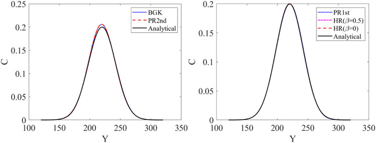
FIGURE 1. Scalar distribution profile for $y=200$ at $t=200$ with Pe = 1 for different collision operators.

FIGURE 2

FIGURE 2. Scalar distribution profile for $y=200$ at $t=200$ with Pe = 1000 for different collision operators.

TABLE 1

TABLE 1. Error comparison for $Pe=1, 1000$ between different collision operators.

4.1.2 Advection-Diffusion of a Rectangular Pulse

In order to test the scalar field LBM with discontinuous initial condition problems, the one-dimensional advection-diffusion of a rectangular pulse is simulated in this section. The simulations are carried out using four different collision operators, BGK, PR1st, PR2nd and HR. Firstly, we make the test without using the filtering method.

The initial rectangular pulse is described as:

$C\left(x,0\right)=\{\begin{array}{cc}1,& 1.5W\ll x\ll 2.5W\\ 0,& otherwise\end{array}(37)$

where $W$ is the pulse width. $L=10\times W$ is the length of computational domain. In this problem, the velocity vector is $u$ and the diffusion coefficient is $D$. The analytical solution of $C$ is given as

$C\left(x,0\right)=\frac{1}{2}\left[erf\left(\frac{2W-x+ut}{2\sqrt{Dt}}\right)+erf\left(\frac{-W+x-ut}{2\sqrt{Dt}}\right)\right](38)$

Here, $erf\left(x\right)=\frac{2}{\sqrt{\pi }}\underset{0}{\overset{x}{{\displaystyle \int }}}{e}^{-{\eta }^2}d\eta$ is the error function.

When the diffusion coefficient of the convection-diffusion equation is relatively large, even if the initial flow field has discontinuous distribution, the discontinuity will become smooth due to the strong dissipation effect of the equation itself. We first take the diffusion coefficient $D=1, 0.1, \text{and} 0.01$, the velocity is $u=0.05$. The results show that the four collision operators achieve almost the same results. Because the differences between analytical, BGK, PR1st, PR2nd and HR ($\beta =0$) collision operators are small, only the results of HR collision operator are given in Figure 3. There is no difference can be seen from the figure, and the errors of the results are further compared in Table 2. We can see that the errors of the results obtained by the four collision operators are basically the same.

FIGURE 3

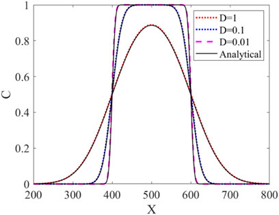
FIGURE 3. Scalar distribution profile for $D=1, 0.1, and 0.01$ at $t=2000$ for the different schemes.

TABLE 2

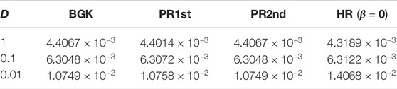
TABLE 2. Error comparison for $D=1, 0.1 and 0.01$ between different collision operators.

If the diffusion coefficient of the convection-diffusion equation is relatively small, when the initial condition has discontinuous, due to the small dissipation effect of the equation itself, oscillation will occur near the discontinuity. In this example, we choose diffusion coefficient $D=1\times e^{-6}$, and the velocity is $u=0.05$. LBM with all the four collision operators BGK, PR1st, PR2nd and HR are tested. Figure 4 shows the concentration profile at $t=2000$. It can be seen that the BGK and PR2nd collision operators obtain almost the same results, which the solution is superimposed with high-frequency waves, but the results of the collision operators in the PR1st form gradually diverge with the calculation. For the HR collision operator, there is no high frequency wave in other regions except for a small overshoot near the discontinuities. It can be seen from Figure 4D that when the $\beta =0.95$, the transition region at the discontinuity is the narrowest.

FIGURE 4

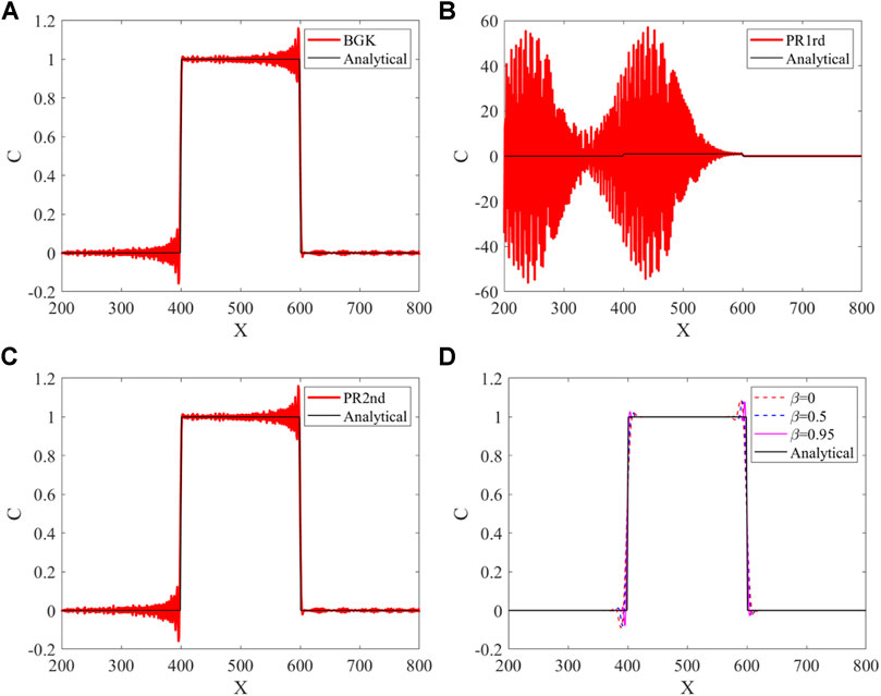
FIGURE 4. Scalar distribution profile for $D=1\times {10}^{-6}$ at $t=2000$ for different schemes: (A) BGK, (B) PR1st, (C) PR2nd, (D) HR.

In order to investigate the influence of the filtering strategy and choose the proper values of ${\sigma }_0$ and $\mathit{ϵ}$, we use the BGK collision operator combined with the filtering method to simulate the advection-diffusion of a rectangular pulse. The diffusion coefficients are taken as $D=1\times e^{-6}$ and $D=1\times e^{-3}$ respectively, and the velocity is $u=0.05$. Specifically, ${\sigma }_0$ and $\mathit{ϵ}$ take the two values of 0.1 and 0.2, so there are four combinations. Scalar distribution profile is shown in Figure 5, we can see that the four sets of filter coefficients can well suppress the oscillation generated at the discontinuity. When the initial discontinuity is transported by convection, its sharp distribution profile is smoothed by the filter, thus reducing the filter intensity coefficient $\sigma$ as depicted in Figure 6. These observations show that the numerical dissipation effects introduced by the dynamical filter with four sets of filter coefficients are similar, with minor differences. When the diffusion coefficient is large, the filter with ${\sigma }_0=0.1$ and $\mathit{ϵ}=0.2$ can be selected, and when the diffusion coefficient is small, the filter with ${\sigma }_0=0.2$ and $\mathit{ϵ}=0.1$ can be selected.

FIGURE 5

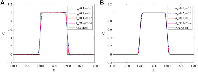
FIGURE 5. Scalar distribution profile for at $t=20000$ for different ${\sigma }_0$ and $\mathit{ϵ}$ (A) $D=1\times {10}^{-6}$ , (B) $D=1\times {10}^{-3}$.

FIGURE 6

FIGURE 6. Time trace of the maximum value of the coefficient $\sigma$ for different ${\sigma }_0$ and $\mathit{ϵ}$ (A) $D=1\times {10}^{-6}$ , (B) $D=1\times {10}^{-3}$.

4.2 Advection-Diffusion in Doubly Periodic Shear Layer Flow

To show the ability of the advection–diffusion LBM and the filtering method, we used a simple test: the scalar transport in doubly periodic shear layer flow. It is a well-known test case which allows to quantify the stability of numerical schemes as a first step [9]. This flow is composed of two longitudinal shear layers, located at $y=L/4$ and $y=3L/4$ , in a 2D doubly periodic domain with $\left(x, y\right)\in {\left[0, L\right]}^2$. The periodic boundaries can avoid additional disturbance from the boundary. A transverse perturbation is superimposed to the flow, leading to the roll-up of the shear layers, and the generation of two counter-rotating vortices by the Kelvin-Helmholtz instability mechanism. We set the initial scalar field along with the flow field, which means that $C=1$ between the shear layers, and in other location $C=0$.

The initial conditions are fully defined through

$u_x=\{\begin{array}{cc}{u}_0\tanh \left[k^{\ast }\left(y^{\ast }-1/4\right)\right],& y^{\ast }\le 1/2\\ u_0\tanh \left[k^{\ast }\left(3/4-y^{\ast }\right)\right],& y^{\ast }\ge 1/2\end{array} (39)$

$u_y=u_0{\delta }^{\ast }\sin \left[2\pi \left(x^{\ast }+1/4\right)\right](40)$

$C=\{\begin{array}{cc}{C}_0\left(1+\tanh \left[k^{\ast }\left(y^{\ast }-1/4\right)\right]\right),& y^{\ast }\le 1/2\\ C_0\left(1+\tanh \left[k^{\ast }\left(3/4-y^{\ast }\right)\right]\right), & y^{\ast }\ge 1/2\end{array}(41)$

where $\left(x^{\ast },y^{\ast }\right)=\left(x/L,y/L\right)$ , and $u_0$ is the characteristic speed. $k^{\ast }$ is related to the width of the shear layers while ${\delta }^{\ast }$ controls the amplitude of the transverse perturbation. The critical parameters of this test case are the width of the shear layers, and the Reynolds number which is the ratio between convective and diffusive phenomena. Here the case of thin shear layers is considered, i.e., $\left(k^{\ast },{\delta }^{\ast }\right)=\left(80, 0.05\right)$. The characteristic speed is $u_0=0.1$. Reynolds number is here fixed to a moderate value of $\text{Re}=u_{0}L/\nu =30000$. The Péclet number is defined by: $\text{Pe}=u_{0}L/D$. It is also useful for the discussion to define the convective time as $t_C=L/u_0$. The flow evolution was simulated up to $t_C$ for various resolutions from 64 × 64 to 512 × 512 Cartesian grid. In this test, the filter strength parameter is selected as ${\sigma }_0=0.2$, and the coefficient of reference gradient norm is taken as $\mathit{ϵ}=0.1$.

4.2.1 Validation of the Velocity Field

In order to validate the flow-field, we successively simulated the rollup of the double shear layer. Both the BGK and the recursive regularization collision operator are used.

Figure 7 presents dimensionless vorticity contours ${\omega }_z/\left|{\omega }_z^{max}\right|$ obtained with the BGK collision operator after one convective time period $t=t_C$. Regarding the coarse mesh grid (128 × 128), numerical oscillations are too strong for the simulation to remain stable. For the fine mesh grid (256 × 256), although the simulation is stable, but there are two spurious secondary vortices are observed. For the finest mesh grid (512 × 512), it does not show any premise of stability issues.

FIGURE 7

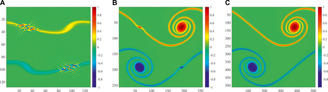
FIGURE 7. Vorticity contours in the double shear layer, for different grids with the BGK collision model. From left to right: 128 × 128, 256 × 256, and 512 × 512.

Figure 8 presents dimensionless vorticity contours obtained with the recursive regularization collision operator after one convective time period $t=t_C$. They all show convergence, despite the inevitable loss of accuracy of the gradients. The algorithm does converge even with the coarsest mesh grid (64 × 64), and there are no spurious secondary vortices. When using the recursive regularization collision operator, the 256 × 256 mesh grid can already obtain relatively accurate flow field information. Therefore, we use this grid resolution to calculate the coupling problem of LBM for fluid mechanics and LBM for scalar transport.

FIGURE 8

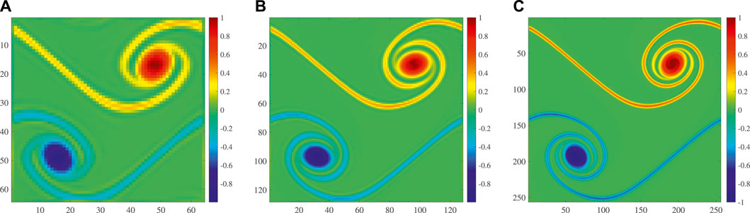
FIGURE 8. Vorticity contours in the double shear layer, for different grids with the recursive regularization collision model. From left to right: 64 × 64, 128 × 128, and 256 × 256.

Furthermore, we compare the velocity fields obtained under the third order and fourth order equilibrium distribution function expansions. The result is given in Figure 9. We can see that the difference between the velocity fields obtained from the third and fourth order expansions is very small.

FIGURE 9

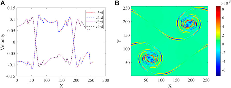
FIGURE 9. Comparison of velocity fields obtained by the third and fourth order expansion of the equilibrium distribution function: (A) velocity profiles along the diagonal lines, (B) contour of the velocity difference.

4.2.2 Tests of Advection-Diffusion of Scalar

In this subsection, the passive scalar transport problem in periodic double shear layer is studied. Because the results obtained by the PR2nd and the BGK are similar, we only give the results of BGK. At first, to better understand the stability of the proposed schemes, the minimum number of grids required for three LBM collision operators that can obtain stable result for different Péclet number are investigated. The flow evolution was simulated up to $t_C$ for three various resolutions 128 × 128, 256 × 256 and 512 × 512 Cartesian grid. The results are given in Table 3.

TABLE 3

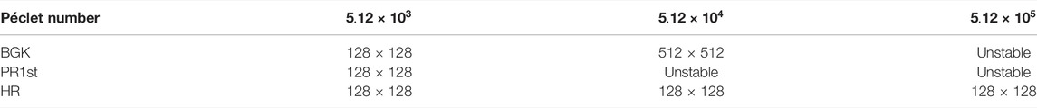
TABLE 3. Grid needed to obtain stable result for different model for given Péclet number.

In the following parts of this section, the passive scalar transport problem in periodic double shear layer is studied in detail with two specific Péclet numbers. The computation grid is 256 × 256, and the velocity field is computed by recursively regularized LBM. The scalar transport equation is solved by using the advection-diffusion LBM with the three collision operators BGK, PR1st and HR respectively. We examine both the medium and extremely large Péclet number regimes.

For comparison, the solution obtained with a classical finite-difference solver is also given. The LBM and FD solver use the same time-step, and first order forward Euler integration is used. Second order central difference operator is used for convection and diffusion.

Since the analytical solution is not available, we take the unfiltered BGK collision operator for a well resolved grid (1024 × 1024) as the reference solution.

4.2.2.1 Test Case With Medium Diffusion Coefficient

First, we consider the case where the equation itself has a medium diffusion coefficient. Here, the diffusion coefficient $D=0.005$ , the corresponding Péclet number is $Pe=5120$. For the case with relatively large diffusion coefficient, even if the filtering method is not used, the finite difference scheme and the LBM with three collision operators can obtain stable results. Figure 10 shows the contours of the scalar distribution of the results calculated by the FD method and the HR collision operator without using the filtering method. Here, the results of PR1st and HR collision operators are basically the same as BGK. For brevity, only the scalar concentration contour of HR is given. It can be seen from the figure that both the FD method and the LBM can well simulate the transport process of the passive scalar along the flow field. The results show that the high gradient regions are distributed smoothly and the details of scalar mixing as the vortex rolls up are well captured. Figure 11A shows the scalar distribution along the counter-diagonal of the computational domain when no filtering method is used. It can be seen that the results of the LBM of the three collision operators are almost identical, and are basically consistent with the results of the FD scheme.

FIGURE 10

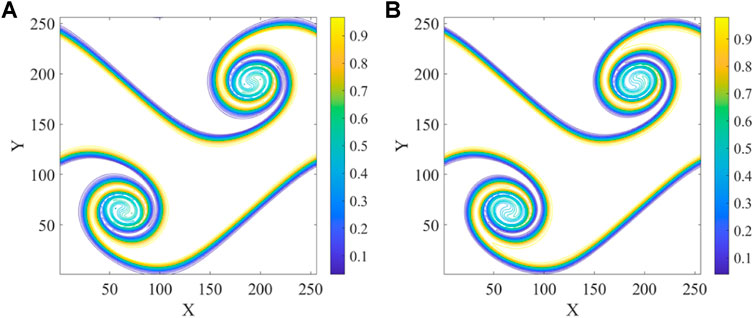
FIGURE 10. Scalar concentration contour plot in the double shear layer at $Pe=5120$ for the FD scheme (A) and HR collision operator (B) without filtering.

FIGURE 11

FIGURE 11. Scalar distribution profile at $Pe=5120$ along the counter-diagonal of the domain for the different schemes: (A) without filter, (B) comparison of results with and without filter.

Next, we consider the effect of using the filtering method on the FD scheme and LBM. Here, because the results of the three collision operators are basically the same, only the HR collision operator is selected as the representative of the LBM. Figure 11B presents a comparison of the scalar distribution along the counter-diagonal of the computational domain with and without the filter. It can be seen that for the example with a relatively large diffusion coefficient, the results using the filtering method are basically consistent with the results without filtering. The adaptive filtering method does not bring significant numerical dissipation.

For a quantitative measure of the error of HR model with and without the filter, the scalar distribution along the counter-diagonal of the computational domain against a reference solution is compared. The L₂ error of the unfiltered HR model is $E_C=4.3537\times {10}^{-2}$, and the L₂ error of the filtered HR model is $E_C=4.7510\times {10}^{-2}$.

Figure 12 shows the filter coefficients contour plot and the distribution profile along the counter-diagonal of the computational domain after using the filter with the FD method and the HR collision operator. We can see the results of the two schemes are basically consistent, and both show good adaptive filtering characteristics.

FIGURE 12

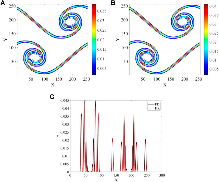
FIGURE 12. Filter coefficient contour plot in the double shear layer at $Pe=5120$: (A) the FD scheme, (B) HR collision operator, and (C) filter coefficient profiles along the counter-diagonal of the domain.

4.2.2.2 Test Case With Small Diffusion Coefficient

We now consider the case where the equation itself has a small diffusion coefficient. Here, the diffusion coefficient $D=5\times {10}^{-8}$ , the corresponding Péclet number is $Pe=5.12\times {10}^8$. In this test, the extremely small value of diffusion coefficient is chosen to highlight the stability issues. For the case with small diffusion coefficient, when the filtering method is not used, whether it is the finite difference scheme or the LBM using any one of the three collision operators, the calculation results have a certain degree of numerical oscillation. The left side of Figure 13 shows the contours of the scalar distribution calculated by the FD scheme and LBM without the filtering method. It can be seen that the LBM with HR collision operator can simulate the transport process of the scalar along the flow field well, although there are small oscillations near the region with high gradient.

FIGURE 13

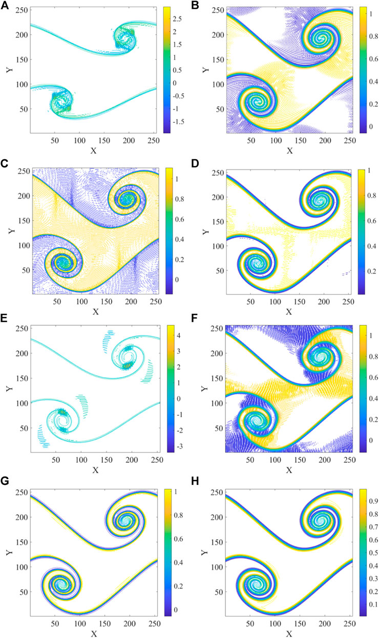
FIGURE 13. Unfiltered (left) and filtered (right) results at $Pe=5.12\times {10}^8$. From top to bottom: (A, B) FD unfiltered and filtered, (C, D) BGK unfiltered and filtered, (E, F) PR1st unfiltered and filtered, (G, H) HR unfiltered and filtered.

For the results of the BGK collision operator, there are high-frequency oscillation waves in almost the entire computational domain. However, the simulation of the FD method and the LBM with PR1st collision operator cannot proceed to one convective time period, and the results tend to diverge. Figure 14 shows the scalar distribution along the counter-diagonal of the computational domain without and with filtering. It can be seen from Figures 14A,C that when the filtering method is not used, the result of LBM with the BGK collision operator has obvious numerical oscillations on the entire curve, while the result of HR collision operator only has a certain overshoot.

FIGURE 14

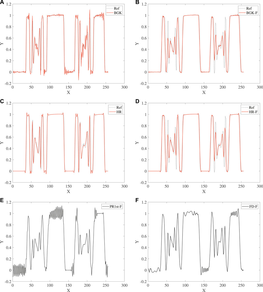
FIGURE 14. Scalar distribution profile at $Pe=5.12\times {10}^8$ along the counter-diagonal of the domain for different schemes: (A,B) BGK unfiltered and filtered, (C,D) HR unfiltered and filtered, (E) PR1st with filter, (F) FD scheme with filter.

After using the filtering method, the stability of both the FD method and the LBM has been improved. The right side of Figure 13 shows the contours of the scalar distribution calculated by the FD scheme and LBM with the filtering method. It can be seen that for the FD method and the PR1st collision operator, the filtering method significantly reduces the magnitude of the numerical oscillation. After using the filtering method, the simulation can be carried out for one convective time period without divergence, but there are still obvious numerical oscillations in the whole computational domain.

It can be seen from Figures 14E,F that when the filtering method is used, scalar distribution along the counter-diagonal of the computational domain of the FD method and the PR1st collision operator still have obvious numerical oscillations. Figures 14A,B show that, for the BGK collision operator, the filtering method can obviously suppress the high frequency oscillation in the computational domain, and a satisfactory result is obtained. For a quantitative measure of the error of BGK model with and without the filter, the scalar distribution along the counter-diagonal of the computational domain against a reference solution is compared. The L₂ error of the unfiltered BGK model is $E_C=2.3644\times {10}^{-1}$, and the L₂ error of the filtered BGK model is $E_C=2.2889\times {10}^{-1}$.

Figures 14C,D show that, for the HR collision operator, the filtering method suppresses the overshoot phenomenon near the region with high gradient and further reduces the amplitude of numerical oscillation. For the HR model with and without the filter, the scalar distribution along the counter-diagonal of the computational domain against a reference solution is compared. The L₂ error of the unfiltered HR model is $E_C=2.1628\times {10}^{-1}$, and the L₂ error of the filtered HR model is $E_C=2.1985\times {10}^{-1}$.

Figure 15 shows the filter coefficients contour plot after using the filter with the FD method and LBM. It can be seen from the figure that for the BGK and HR collision operators the distribution of the filter coefficients is very smooth, and the filtering method only has an obvious effect in the scalar mixing region in the shear layer. This is principally because the scalar component distributions of the BGK and HR collision operators are relatively smooth. For the FD method and the PR1st collision operator, since there are obvious numerical oscillations in the computational domain, the filter coefficients also have obvious distributions in the flow region outside the shear layer.

FIGURE 15

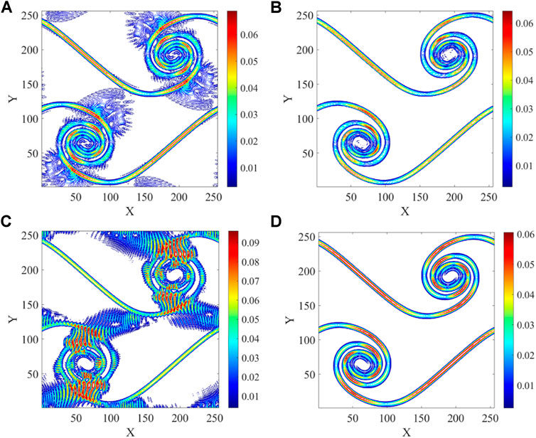
FIGURE 15. Filter coefficient contour plot in the double shear layer at $Pe=5.12\times {10}^8$ for different schemes: (A) FD scheme, (B) BGK collision operator, (C) PR1st collision operator, (D) HR collision operator.

5 Conclusion

The advection-diffusion lattice Boltzmann models with BGK, PR1st, PR2nd and HR collision operators for scalar transport in uniform and complex flow are tested. In addition, an adaptive dynamic filtering method with a filter coefficient based on the gradient of the transport scalar is also tested. Mass and momentum conservation are addressed within a lattice Boltzmann flow solver, whereas the scalar conservation is addressed via the advection-diffusion lattice Boltzmann models. In the test of scalar transport in uniform flow, the LBM with PR2nd collision operator obtains almost the same result as the BGK collision operator, which both have significant errors when the diffusion coefficient is large in the test of Gaussian hill and have similar high frequency oscillation when the diffusion coefficient is small in the test of rectangular pulse. In its stability range, the accuracy of the PR1st collision operator is similar to that of the HR, but there will be serious numerical oscillation in the case of rectangular pulse with small diffusion coefficient. In the test of advective-diffusion in complex flow, we can see that, for the case with medium diffusion coefficient, the results of the LBM with the different collision operators are almost identical, and are basically consistent with the results of the FD scheme. However, when the diffusion coefficient is extremely small, the different collision operators and the FD scheme have different performances. The LBM with BGK collision operator can obtain a result with high-frequency oscillation waves in the domain. The simulation of the FD method and the LBM with PR1st collision operator cannot obtain stable results. The transport process of the scalar along the flow field can be simulated well by the LBM with HR collision operator. Introducing a local filter such as the one proposed in this study stabilizes the simulations of both LBM and FD scheme. Then for the simulation of high Péclet number flow, the dynamical filtering strategy should be seen as an enhanced stabilization procedure for the lattice Boltzmann method where the amount of numerical dissipation is locally controlled in space.

Data Availability Statement

The original contributions presented in the study are included in the article/Supplementary Material, further inquiries can be directed to the corresponding author.

Author Contributions

ZZ: Conceptualization, methodology, software, investigation, writing—original draft. ZL: Supervision, Methodology. YW: Supervision, writing—review and editing.

Funding

This work was supported by the Advanced Jet Propulsion Innovation Center, AEAC (Project ID. ZZCX-2020-004). The authors declare that this study received funding from AEAC, Aero Engine Academic of China, Aero Engine Corporation of China (AECC). The funder was not involved in the study design, collection, analysis, interpretation of data, the writing of this article or the decision to submit it for publication.

Conflict of Interest

Author YW was employed by company Aero Engine Academic of China, Aero Engine Corporation of China (AECC).

The remaining authors declare that the research was conducted in the absence of any commercial or financial relationships that could be construed as a potential conflict of interest.

Publisher’s Note

All claims expressed in this article are solely those of the authors and do not necessarily represent those of their affiliated organizations, or those of the publisher, the editors and the reviewers. Any product that may be evaluated in this article, or claim that may be made by its manufacturer, is not guaranteed or endorsed by the publisher.

References

1. Guo Z, Shu C. Lattice Boltzmann Method and its Applications in Engineering. Singapore: World Scientific (2013).

Google Scholar

2. Huang H, Sukop M, Lu X. Multiphase Lattice Boltzmann Methods: Theory and Application. Oxford: John Wiley & Sons (2015).

Google Scholar

3. Succi S. The Lattice Boltzmann Equation: For Complex States of Flowing Matter. Oxford: Oxford University Press (2018).

Google Scholar

4. Fei L, Luo KH, Lin C, Li Q. Modeling Incompressible Thermal Flows Using a Central-Moments-Based Lattice Boltzmann Method. Int J Heat Mass Transf (2018) 120:624–34. doi:10.1016/j.ijheatmasstransfer.2017.12.052

CrossRef Full Text | Google Scholar

5. Fattahi E, Farhadi M, Sedighi K, Nemati H. Lattice Boltzmann Simulation of Natural Convection Heat Transfer in Nanofluids. Int J Therm Sci (2012) 52:137–44. doi:10.1016/j.ijthermalsci.2011.09.001

CrossRef Full Text | Google Scholar

6. Guo Z, Zhao TS. A Lattice Boltzmann Model for Convection Heat Transfer in Porous Media. Numer Heat Transf Part B Fundam (2005) 47(2):157–77. doi:10.1080/10407790590883405

CrossRef Full Text | Google Scholar

7. Hosseini SA, Eshghinejadfard A, Darabiha N, Thévenin D. Weakly Compressible Lattice Boltzmann Simulations of Reacting Flows with Detailed Thermo-Chemical Models. Comput Math Appl (2020) 79(1):141–58. doi:10.1016/j.camwa.2017.08.045

CrossRef Full Text | Google Scholar

8. Hosseini SA, Darabiha N, Thévenin D. Mass-Conserving Advection-Diffusion Lattice Boltzmann Model for Multi-Species Reacting Flows. Phys A Stat Mech its Appl (2018) 499:40–57. doi:10.1016/j.physa.2018.01.034

CrossRef Full Text | Google Scholar

9. Dellar PJ. Bulk and Shear Viscosities in Lattice Boltzmann Equations. Phys Rev E Stat Nonlin Soft Matter Phys (2001) 64:031203. doi:10.1103/PhysRevE.64.031203

PubMed Abstract | CrossRef Full Text | Google Scholar

10. David C, Sagaut P. Structural Stability of Lattice Boltzmann Schemes. Phys A Stat Mech its Appl (2016) 444:1–8. doi:10.1016/j.physa.2015.09.089

CrossRef Full Text | Google Scholar

11. Wissocq G, Sagaut P, Boussuge J-F. An Extended Spectral Analysis of the Lattice Boltzmann Method: Modal Interactions and Stability Issues. J Comput Phys (2019) 380:311–33. doi:10.1016/j.jcp.2018.12.015

CrossRef Full Text | Google Scholar

12. Masset PA, Wissocq G. Linear Hydrodynamics and Stability of the Discrete Velocity Boltzmann Equations. J Fluid Mech (2020) 897. doi:10.1017/jfm.2020.374

CrossRef Full Text | Google Scholar

13. Coreixas C, Wissocq G, Chopard B, Latt J. Impact of Collision Models on the Physical Properties and the Stability of Lattice Boltzmann Methods. Phil Trans R Soc A (2020) 378(2175):20190397. doi:10.1098/rsta.2019.0397

PubMed Abstract | CrossRef Full Text | Google Scholar

14. Hosseini SA, Coreixas C, Darabiha N, Thévenin D. Stability of the Lattice Kinetic Scheme and Choice of the Free Relaxation Parameter. Phys Rev E (2019) 99:063305. doi:10.1103/PhysRevE.99.063305

PubMed Abstract | CrossRef Full Text | Google Scholar

15. Wissocq G, Coreixas C, Boussuge JF. Linear Stability and Isotropy Properties of Athermal Regularized Lattice Boltzmann Methods. Phys Rev E (2020) 102(5):053305. doi:10.1103/PhysRevE.102.053305

PubMed Abstract | CrossRef Full Text | Google Scholar

16. Wissocq G, Sagaut P. Hydrodynamic Limits and Numerical Errors of Isothermal Lattice Boltzmann Schemes. J Comput Phys (2022) 450:110858. doi:10.1016/j.jcp.2021.110858

CrossRef Full Text | Google Scholar

17. Renard F, Wissocq G, Boussuge J-F, Sagaut P. A Linear Stability Analysis of Compressible Hybrid Lattice Boltzmann Methods. J Comput Phys (2021) 446:110649. doi:10.1016/j.jcp.2021.110649

CrossRef Full Text | Google Scholar

18. Suga S. Numerical Schemes Obtained from Lattice Boltzmann Equations for Advection Diffusion Equations. Int J Mod Phys C (2006) 17(11):1563–77. doi:10.1142/s0129183106010030

CrossRef Full Text | Google Scholar

19. Hosseini SA, Darabiha N, Thévenin D, Eshghinejadfard A. Stability Limits of the Single Relaxation-Time Advection-Diffusion Lattice Boltzmann Scheme. Int J Mod Phys C (2017) 28(12):1750141. doi:10.1142/s0129183117501418

CrossRef Full Text | Google Scholar

20. d’Humière D, Ginzburg I, Krafczyk Y, Lallemand P, Luo L. Multiple Relaxation Time Lattice Boltzmann Models in Three Dimensions. Philosophical Trans R Soc Lond. Ser A Math Phys Eng Sci (2002) 360(1792):437–51. doi:10.1098/rsta.2001.0955

CrossRef Full Text | Google Scholar

21. Latt J, Chopard B. Lattice Boltzmann Method with Regularized Pre-collision Distribution Functions. Math Comput Simul (2006) 72(2-6):165–8. doi:10.1016/j.matcom.2006.05.017

CrossRef Full Text | Google Scholar

22. Tosi F, Ubertini S, Succi S, Chen H, Karlin I. Numerical Stability of Entropic Versus Positivity-Enforcing Lattice Boltzmann Schemes. Math Comput Simul (2006) 72(2-6):227–31. doi:10.1016/j.matcom.2006.05.007

CrossRef Full Text | Google Scholar

23. Malaspinas O, Sagaut P. Advanced Large-Eddy Simulation for Lattice Boltzmann Methods: The Approximate Deconvolution Model. Phys Fluids (2011) 23(10):105103. doi:10.1063/1.3650422

CrossRef Full Text | Google Scholar

24. Ricot D, Marié S, Sagaut P, Bailly C. Lattice Boltzmann Method with Selective Viscosity Filter. J Comput Phys (2009) 228(12):4478–90. doi:10.1016/j.jcp.2009.03.030

CrossRef Full Text | Google Scholar

25. Nathen P, Haussmann M, Krause MJ, Adams NA. Adaptive Filtering for the Simulation of Turbulent Flows with Lattice Boltzmann Methods. Comput Fluids (2018) 172:510–23. doi:10.1016/j.compfluid.2018.03.042

CrossRef Full Text | Google Scholar

26. Marié S, Gloerfelt X. Adaptive Filtering for the Lattice Boltzmann Method. J Comput Phys (2017) 333:212–26. doi:10.1016/j.jcp.2016.12.017

CrossRef Full Text | Google Scholar

27. Grad H. On the Kinetic Theory of Rarefied Gases. Comm Pure Appl Math (1949) 2(4):331–407. doi:10.1002/cpa.3160020403

CrossRef Full Text | Google Scholar

28. Guo Z, Zheng C, Shi B. Discrete Lattice Effects on the Forcing Term in the Lattice Boltzmann Method. Phys Rev E Stat Nonlin Soft Matter Phys (2002) 65:046308. doi:10.1103/PhysRevE.65.046308

PubMed Abstract | CrossRef Full Text | Google Scholar

29. Li X, Shan X. Self-Consistent Force Scheme in the Discrete Boltzmann Equation. arXiv preprintarXiv:1812.10603 (2018).

Google Scholar

30. Malaspinas O. Increasing Stability and Accuracy of the Lattice Boltzmann Scheme: Recursivity and Regularization. arXiv preprint arXiv:1505.06900 (2015).

Google Scholar

31. Chopard B, Falcone JL, Latt J. The Lattice Boltzmann Advection-Diffusion Model Revisited. Eur Phys J Spec Top (2009) 171(1):245–9. doi:10.1140/epjst/e2009-01035-5

CrossRef Full Text | Google Scholar

32. Wang L, Shi B, Chai Z. Regularized Lattice Boltzmann Model for a Class of Convection-Diffusion Equations. Phys Rev E Stat Nonlin Soft Matter Phys (2015) 92(4):043311. doi:10.1103/PhysRevE.92.043311

PubMed Abstract | CrossRef Full Text | Google Scholar

33. Coreixas C, Wissocq G, Puigt G, Boussuge JF, Sagaut P. Recursive Regularization Step for High-Order Lattice Boltzmann Methods. Phys Rev E (2017) 96(3):033306. doi:10.1103/PhysRevE.96.033306

PubMed Abstract | CrossRef Full Text | Google Scholar

34. Jonnalagadda A, Sharma A, Agrawal A. Onsager-Regularized Lattice Boltzmann Method: A Nonequilibrium Thermodynamics-Based Regularized Lattice Boltzmann Method. Phys Rev E (2021) 104(1):015313. doi:10.1103/PhysRevE.104.015313

PubMed Abstract | CrossRef Full Text | Google Scholar

35. Latt J, Chopard B, Malaspinas O, Deville M, Michler A. Straight Velocity Boundaries in the Lattice Boltzmann Method. Phys Rev E Stat Nonlin Soft Matter Phys (2008) 77(5):056703. doi:10.1103/PhysRevE.77.056703

PubMed Abstract | CrossRef Full Text | Google Scholar

36. Skordos PA. Initial and Boundary Conditions for the Lattice Boltzmann Method. Phys Rev E (1993) 48:4823–42. doi:10.1103/physreve.48.4823

CrossRef Full Text | Google Scholar

37. Chai Z, Shi B. Multiple-Relaxation-Time Lattice Boltzmann Method for the Navier-Stokes and Nonlinear Convection-Diffusion Equations: Modeling, Analysis, and Elements. Phys Rev E (2020) 102(2):023306. doi:10.1103/PhysRevE.102.023306

PubMed Abstract | CrossRef Full Text | Google Scholar

38. Jacob J, Malaspinas O, Sagaut P. A New Hybrid Recursive Regularized Bhatnagar–Gross–Krook Collision Model for Lattice Boltzmann Method-Based Large Eddy Simulation. J Turbul (2018) 19(11-12):1051–76. doi:10.1080/14685248.2018.1540879

CrossRef Full Text | Google Scholar

39. Tam CKW, Webb JC, Dong Z. A Study of the Short Wave Components in Computational Acoustics. J Comp Acous (1993) 01(01):1–30. doi:10.1142/s0218396x93000020

CrossRef Full Text | Google Scholar