Memory Behaviors of Air Pollutions and Their Spatial Patterns in China

Particulate matter (PM_2.5 and PM₁₀) and ozone (O₃) are the two major air pollutants in China in recent years. The fluctuations of PM_2.5, PM₁₀ and O₃ strongly depend on the weather processes and anthropogenic emission. These processes may lead to the existence of short- and long-term memory behaviors in air pollutants. Hence, here we use the autoregressive parameter a of the first-order autoregressive process [AR (1)] to characterize the short-term memory effects of pollutants. We estimate the scaling exponent α using detrended fluctuation analysis (DFA) for the long-term memory effects of air pollutants (PM_2.5, PM₁₀, and O₃) in summer and winter for different cities in China. Our results show that PM_2.5, PM₁₀, and O₃ have strong short-term and long-term memory characteristics both in summer and winter. Furthermore, both the short- and long-term memory effects are stronger in winter than summer for most cities associated with stronger and longer persistent weather systems in winter. In general, the scaling exponent α of PM_2.5 and PM₁₀ are smaller for northern cities than those of southern cities in China. The long-term memory patterns of O₃ are stronger in northern cities and weaker in southern cities in relative to those of PM_2.5 and PM₁₀ in winter. Our results show that the short- and long-term memory behaviors of air pollutions are dominated by the weather systems with different time scales.

Introduction

In recent decades, air pollution as a by-product of increased industrialization and urbanization, has been highly valued by the public and local government agencies in China. Air pollution regulation, air quality forecast and other related works have become critical issues to scientific researchers [1]. The sources of atmospheric pollutants are divided into natural and anthropogenic [2]. Anthropogenic sources include carbon and organic compounds emitted from heavy industries such as electric power, metal smelting and non-metallic mineral products, or emitted from the motor exhaust gas and coal combustion [3]. During 2013–2017, Beijing and other cities in north China suffered severe and persistent haze events caused by high fine particulate matter (PM_2.5) concentrations [4]. The Chinese State Council issued powerful policies to restrict pollution emissions [5]. So far, PM_2.5 concentrations have been reduced by 30% in China [5]. However, ozone (O₃) concentrations show an increasing trend in recent years [6]. PM_2.5 and O₃ have been the two major air pollutants in most Chinese cities. Direct or indirect exposure to air pollutions PM_2.5 and O₃ can seriously damage our physical and mental health, causing respiratory infections, various contact allergies and other diseases [7].

Time dependence and temporal predictability of time series are associated with memory behavior of time series. Nature time series such as earthquake and climate records have been found to widely exit the memory behavior [8–10]. A short-term memory process can be expressed by a first-order autoregressive process and quantified by fitting the parameter of AR (1) [11]. For nature time series, usually both short and long-term memory processes exit. Yuan et al. [12] showed that Antarctic sea ice extent is not a simple short-term persistence time series, but is actually a combination of short- and long-term memory processes. To quantify such long-term memory of time series, Peng et al. [13] proposed Detrended Fluctuation Analysis (DFA) under the fractal theory [14, 15] for the first time to study the memory behavior of internal molecular chains of DNA. This method can filter out the trend component of its own evolution, and the remaining deviation sequence is the component of its own fluctuation [16–19]. Thus, it can eliminate the unreal correlation caused by the non-stationary characteristics of time series [20]. The DFA method has been successfully applied to seismology, stock market, biology, climate and environment, etc. [21–24]. For example, Lennartz et al. [25] and Fan et al. [23] used the DFA method to find that the memory exists in inter-occurrence seismic records. Yang et al. [26] estimate the persistence of precipitation over a wider range of scales and show that precipitation persistence can be described as a varying by DFA. Yuan et al. [27] observed temperature records of 12 stations from Antarctica island, coastline, and continental areas are analyzed by means of DFA and they found different long-term climate memory (LTM) behaviors.

Also, previous studies have found significant long-term (short-term) memory in air pollutant concentrations in some regions [28–30]. Liu et al. [31] found that there are different self–organized criticality process for pollutions SO₂, NO₂, and PM₁₀ and the daily air pollution indices (API) associated with different power–law relations in Shanghai by using DFA and multifractal method. Also, Shi et al. [32] showed that the time series of three pollution indexes (SO₂, NO₂, and PM₁₀) and the daily air pollution indexes (APIs) in China have a strong long-term memory within a year by three different methods. For other countries, the similar long-term memory behaviors of air pollution were also found i.e., Nikolopoulos et al. [33] used DFA to analyze PM₁₀ time series in the Athens area (GAA) and found the long-memory patterns. Windsor et al. [34] examined the statistical characteristics of United Kingdom pollution time series and found evidences of high persistence and long-term memory of pollutant fluctuations up to 400 days. PM₁₀ and O₃ pollutants in the Caribbean region showed the multifractal nature with the significant Hurst parameter [35]. Wu et al. [36] studied the long-term persistence characteristics of several air pollutants (PM_2.5 and O₃) during the epidemic situation of COVID-19 by using multifractal detrended fluctuation analysis (MFDFA) and they found that the concentrations of three cities (Changsha, Zhuzhou, and Xiangtan) showed strong long-term persistence characteristics and multifractal structures. Shi et al. [37] comparatively analyzed the long-term persistence characteristics of PM_2.5 evolution for eight air monitoring stations of Chengdu and the results showed that the spatial and temporal evolution of PM_2.5 exhibit a long-term persistence. However, the above studies did not involve the spatial and temporal distribution characteristics of short- and long-term memory of air pollutants over China. In this paper, the DFA method is introduced to study the spatial evolution characteristics of memory of three pollutants (PM_2.5, PM₁₀, and O₃) in 366 cities of China. Moreover, we compare the memory behaviors between short- and long-term scales.

The structure of this paper is as follows: in Section 2, the source of air pollution data and the data processing method are described. In Section 3, we give the specific steps of eliminating DFA method. Section 4 shows the results. Section 5 further summarizes our findings and draws the conclusion.

Data

Hourly time series of three air pollutants concentrations (PM_2.5, PM₁₀, O₃) in 366 Chinese cities are downloaded from the website (https://quotsoft.net/air/). The time period is from 2015 to 2020. In this paper, we focus on air pollution concentrations in winter and summer over China. Here, we define November, December, January, and February as winter; and May, June, July, and August are defined as summer. The lengths of PM_2.5, PM₁₀, and O₃ time series in winter and summer are shown in Table 1.

TABLE 1

TABLE 1. Summary of PM_2.5, PM₁₀, and O₃ concentration data.

Methods

First of all, we remove the seasonal and daily trend from the original data, which can be represented as X $(h,d,y)$ as a function of hour $h$, day $d$, and year $y$. The method to obtain detrend data X $\text{'}(h,d,y)$ is as follows:

$X^{\prime }\left(h,d,y\right)=X\left(h,d,y\right)-\overline{X}\left(h,d\right)(1)$

$\overline{X}\left(h,d\right)=\frac{1}{66}{\displaystyle \sum }_{d_0=-5}^5{\displaystyle \sum }_{y=2015}^{2020}X\left(h,d+d_0,y\right)(2)$

where $\overline{X}(h,d)$ represents the averaged seasonal and daily trend at day $d$ and hour $h$. Since there are some missing data in the original data, we use the linear interpolation method to fill the missing data. The arithmetic mean of the previous and next neighbors’ concentration to the vacancy position is used to supplement the missing data to ensure the integrity and continuity of the data.

Short- and long-term correlated time series can be well described as a generalized AR (1) [12]:

${X^{\prime }}_H=a{X^{\prime }}_{H-1}+{\epsilon }_{\alpha } (3)$

where H is order of time step and a is the parameter of the first-order autoregressive process. The short-term memory of time series can be characterized by the parameter a. We can obtain the parameter a according to the least square method to estimate the AR (1) process of the detrended time series of pollution data [38]. ${\epsilon }_{\alpha }$ is the long-term correlated noise with Hurst index $\alpha$, which characterizes the long-term memory of time series. The parameter is the DFA scale exponent can be obtained as follows.

In general, the DFA algorithm can be divided into five steps [26]:

1) For the detrended time series $X_i\prime$ $(i=\mathrm{1,2...}, N)$, we calculate its cumulative deviation sequence $y\left(k\right)$:

$y\left(k\right)={\displaystyle \sum }_{i=1}^k\left(X_i^{\prime }-\left(X^{\prime }\right)\right), k=\mathrm{1,2},\mathrm{...},N(4)$

where N is the total length of the time series, $X\prime$ is the average of the time series.

2) Then we divide the sequence $y\left(k\right)$ into n new data segments j $(j=1, 2,\mathrm{..}n)$, where $n=int(N/t)$ (the “int” means to obtain integer processing for the value of N/t) and $t$ is the length of each segment $j$. Since $N$ is not always divisible by $t$, the same segmentation operation is performed on the time series $y\left(k\right)$ from back to front as well as from front to back, so that $2n$ segments (length $t$) are obtained.

3) We then obtained the regression of fitting trends $V_j^m\left(k\right)$ by least square method for each segment, where $m$ is the order of regression trend. Here we take the regression trend order $m=2$. Then we calculate the sequence of each segment after eliminating the trend, expressed as: $y_j\left(k\right)=y\left(k\right)-V_j^m\left(k\right).$ The mean variance of each segment after $y_j\left(k\right)$ segmentation can be calculated by the following Eqs. 5, 6. The variance of each segment $j$ obtained for dividing the time series $y\left(k\right)$ from front to back is:

$F^2\left(j,t\right)=\frac{1}{t}{\displaystyle \sum _{i=1}^t{\left[y\left(\left(j-1\right)t+i\right)-V_j^m\left(\left(j-1\right)t+i\right)\right]}^2}j=\mathrm{1,2},\mathrm{...},n(5)$

and from back to front is:

$F^2\left(j,t\right)=\frac{1}{t}{\displaystyle \sum _{i=1}^t{\left[y\left(N-\left(j-n\right)t+i\right)-V_j^m\left(N-\left(j-n\right)t+i\right)\right]}^2}j=n+1,n+2,\mathrm{...},2n (6)$

4) The fluctuation function $F\left(t\right)$ is obtained by averaging the variance for both from front to back and from back to front as:

$F\left(t\right)={\left[\frac{1}{2n}{\displaystyle \sum _{j=1}^{2n}{F}^2\left(j,t\right)}\right]}^{1/2 }(7)$

5) Taking different time scales $t$ and repeating steps 2 to 4, we can obtain $F\left(t\right)$ under different time scales $t$. The fluctuation $F\left(t\right)$ as a function of $t$ is assumed to satisfy a power-law relation: $F\left(t\right)\propto t^{\alpha }$, where $\alpha$ is a scale exponent (also known as the DFA index). Scale exponent $\text{α}$ is an important index to reflect the long-term correlation characteristics of time series and a quantitative index to measure the “balance” degree of time scale [39]. When $0<\alpha <1/2$ , the sequence shows anti-correlation, and this correlation will increase with the decrease of $\alpha$. When $1/2<\alpha <1$, the sequence shows a persistent long-range power-law correlation, and the correlation is stronger with the increase of $\alpha$. When $\alpha =1/2$ , the sequence has no correlation and is random. When $\alpha >1$ , the sequence is long-range correlated, but not power-law correlated.

Results

First, we show samples of the detrended times series of PM_2.5, PM₁₀, and O₃ concentrations as Eq. 1 for Beijing, Shanghai, Chengdu, and Guangzhou in Figure 1. There are larger fluctuations for PM_2.5 and PM₁₀ than other cities, especially in winter as shown in Figure 1A. Due to the implementation of environmental protection policies of China in recent years, we can clearly see that the fluctuation of PM_2.5 is smaller in recent years in comparison to that of the earlier years. In Figure 1C, Guangzhou shows the smallest fluctuation for the PM pollution than other cities. This fluctuation can be strongly affected by meteorological factors [40–43]. The meteorological field is generally more intense in Northern China than Southern China. For the O₃ times series, it shows completely different features with PM. The largest O₃ fluctuation appears in summer related to the product of photochemical reactions. Furthermore, the O₃ fluctuation seems to be more intense in Guangzhou than other cities. Also, the detrended O₃ fluctuation does not show a significant increasing or decreasing trend with time for these four cities in Figure 1. Though the seasonal and daily cycles have been removed for the times series, we can still observe the large different characteristics between winter and summer such that we consider below the memory behaviors for winter and summer, respectively.

FIGURE 1

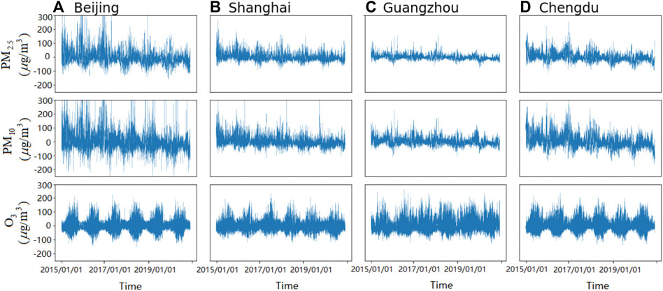
FIGURE 1. Samples of detrended time series of hourly PM_2.5, PM₁₀, and O₃ concentrations for (A) Beijing, (B) Shanghai, (C) Guangzhou, and (D) Chengdu, respectively. The time span is from 2015.01.01 to 2020.12.31.

Next, we use the least square method to estimate the AR (1) process of the detrended time series of PM_2.5, PM₁₀, and O₃ to obtain the autoregressive parameter a in Eq. 3. We show the spatial distribution of the autoregressive parameter a of 366 Chinese cities for summer and winter respectively in Figure 2. By comparing the autoregression parameters a of PM_2.5, PM₁₀, and O_3, we find that the short-term memory effects of pollutants have seasonal and regional differences. And the short-term scale is hour-to-hour. For summer, particulate matters in central and eastern China show stronger short-term memory behavior, especially around the Sichuan Basin and Hubei Province. The values of individual cities are as high as 0.98. For most winter cites, the short-term memory effects of PM_2.5 and PM₁₀ were stronger than those shown in the summer. Compared with PM_2.5 and PM_10, the short-term memory of O₃ varies less, and the a value is stable at around 0.9 or lower in different regions and seasons. The results suggest that compared with O₃, PM_2.5, and PM₁₀ are more dependent on the local meteorological conditions, which strongly influenced by the short-term memory behavior. In winter, the meteorological conditions are stronger and the boundary layer is lower than in summer leading to the stronger short-term memory behaviors of PM_2.5 and PM₁₀. The higher value of a with stronger short memory in PM_2.5 and PM₁₀ over southeast China corresponds to higher intrinsic predictability [44]. Studies also show that other meteorological variables over southeast China exhibit higher intrinsic predictability [45]. The results also show the contrast performance of a-values in South and North China, which will be discussed further in later chapters.

FIGURE 2

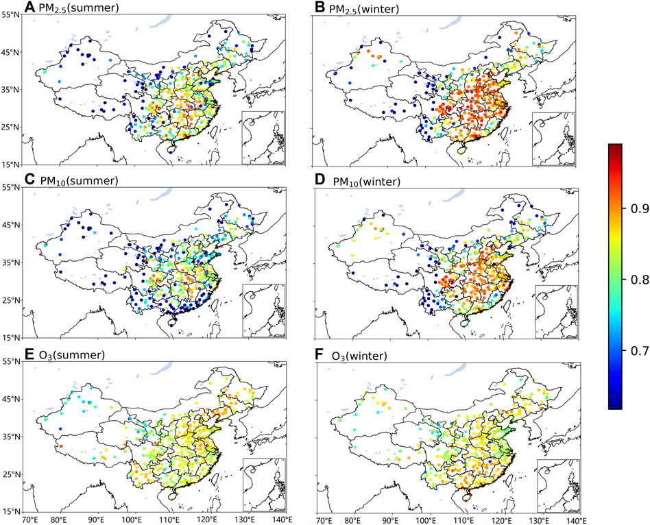
FIGURE 2. (color online) Spatial distributions of the autoregression parameter a for AR (1) process for (A) PM_2.5, (C) PM₁₀ and (E) O₃ in summer. (B), (D), and (F) are same as (A), (C), and (D) but in winter.

Then, we study the long-term memory of pollutions and implement the DFA analysis to the detrended time series of PM_2.5, PM₁₀, and O₃ for the four cities. And the long-term scale is month-to-month. According to Eq. 7, we can obtain the fluctuation F(t) as a function of time scale t for summer (see Figure 3). Previous studies [46, 47] pointed out that due to the effect of limited length of time series, the beginning part of F(t) may be affected by short-term memory effect and lead to a overestimated DFA index. For the AR (1) process, the reliable time scale t to fit scale index $\text{α}$ should be above the crossover $s_x=\frac{15a}{(1-a)(1+a)}$ (a is the parameter of AR (1) process) theoretically [46]. We calculate the crossover s_x and plot in Figure 2 (Red dashed lines). Indeed, the short time scale range below s_x shows some different scale behaviors with that above s_x in Figure 2 which is affected by the short-term memory effect. Thus, we only fit scale exponent $\text{α}$ for the time scale t above the crossover s_x. Here we show the results of four typical cities, and further summarize the DFA scaling exponent α in Table 2. For the four cities, they all show $1/2<\alpha <1$ with the strong long-term memory. In summer, all DFA index $\alpha$ are higher than 0.7, except for Beijing $\alpha =$ 0.66 for PM_2.5. In summer, the boundary lay is high so that it benefits to the diffusion of air pollution, especially in Beijing.

FIGURE 3

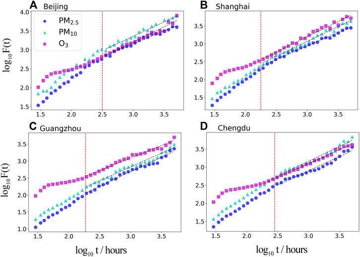
FIGURE 3. (color online) The DFA analysis in summer for (A) Beijing, (B) Shanghai, (C) Guangzhou, and (D) Chengdu. Black dashed lines are fitted power-law curves. Red dashed lines represents the location of the crossover point $s_x$ of AR (1) processes with different parameters a.

TABLE 2

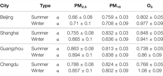
TABLE 2. The DFA scale index $\text{α}$ of PM_2.5, PM₁₀, and O₃ for Beijing, Shanghai, Guangzhou, and Chengdu in summer and winter respectively.

We show the results of winter in Figure 4. There are clear differences between the time scales below and above s_x. The index $\text{α}$ values of four cities show stronger long-term memory effect in winter. We find that except for PM_2.5 and PM₁₀ in Shanghai, the $\text{α}$ values of the other three cities are higher than 0.7 in winter (see Table 2). The memory of pollutants in winter is stronger associated with more persistent weather systems in general. But Shanghai is different, which is located on the west coast of the Pacific Ocean and belongs to the subtropical marine monsoon climate. Compared with summer, the persistent low temperature and northerly wind in winter in Shanghai [48]. They couple with the increase of local emission sources and frequent cold air activities and other meteorological factors, leading to the intensification of pollutant concentration changes. Therefore, these factors may lead to lower persistent characteristics of PM concentrations in winter for Shanghai.

FIGURE 4

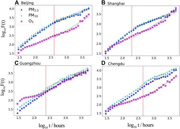
FIGURE 4. (color online) The DFA analysis in winter for (A) Beijing, (B) Shanghai, (C) Guangzhou and (D) Chengdu. Black dashed lines are fitted power-law curves. Red dashed lines represents the location of the crossover point $s_x$ of AR (1) processes with different parameters a.

To comprehensively understand spatial patterns of the memory of pollutants in China, we further study the spatial distribution of the DFA index $\text{α}$ for PM_2.5, PM₁₀, and O₃ in 366 Chinese cities. We repeat the above DFA analysis to obtain the index $\text{α}$ for each city. The spatial distributions of $\text{α}$ are presented in Figure 5 for summer and winter respectively. We find that the scale exponent $\text{α}$ of most cities is between 0.7 and 1 in summer and winter, indicating that the three pollutants in Chinese cities have strong long-term memory. There are largest $\text{α}$ values located in Central and Eastern China for PM_2.5 and PM₁₀ in Figures 5A–D. Moreover, Northern China has a smaller $\text{α}$ value than Southern China for PM_2.5 and PM₁₀ and summer has a smaller $\text{α}$ value than winter for PM_2.5, PM₁₀, and O₃. The cause of long-term memory difference between north and south might be the influence of long-term meteorological factors. For winter, the largest $\alpha$ value with strongest memory locates in the Sichuan basin for Figures 5B,D of PM_2.5 and PM₁₀. In the basin, the stable temperature inversion and low boundary layer are easy to be formed in winter leading to the accumulation of PM_2.5 and PM₁₀ on surface and causing the long-persistent haze Meteorological conditions related to PM_2.5 and PM₁₀ have been found to be different between Northern China and Southern China, i.e., Zhang et al. found that the Rossby waves can influence PM_2.5 in Northern China but not Southern China [43]; relative humidity in Northern and Southern China is positive and negative correlated with PM_2.5 respectively [49]. Moreover, strong northwest winds and cold fronts can rapidly disperse the PM pollutants leading to the lower memory in Northern China. In general, the memory of PM pollutants in winter is stronger than in summer. The temperature decreases significantly due to nighttime radiation. If the surface atmospheric temperature is lower than the upper atmospheric temperature, the inversion layer will form [50]. This prevents convection up and down the air, making it difficult for pollutants to accumulate in winter. And the air pollution caused by coal consumption is more serious in winter.

FIGURE 5

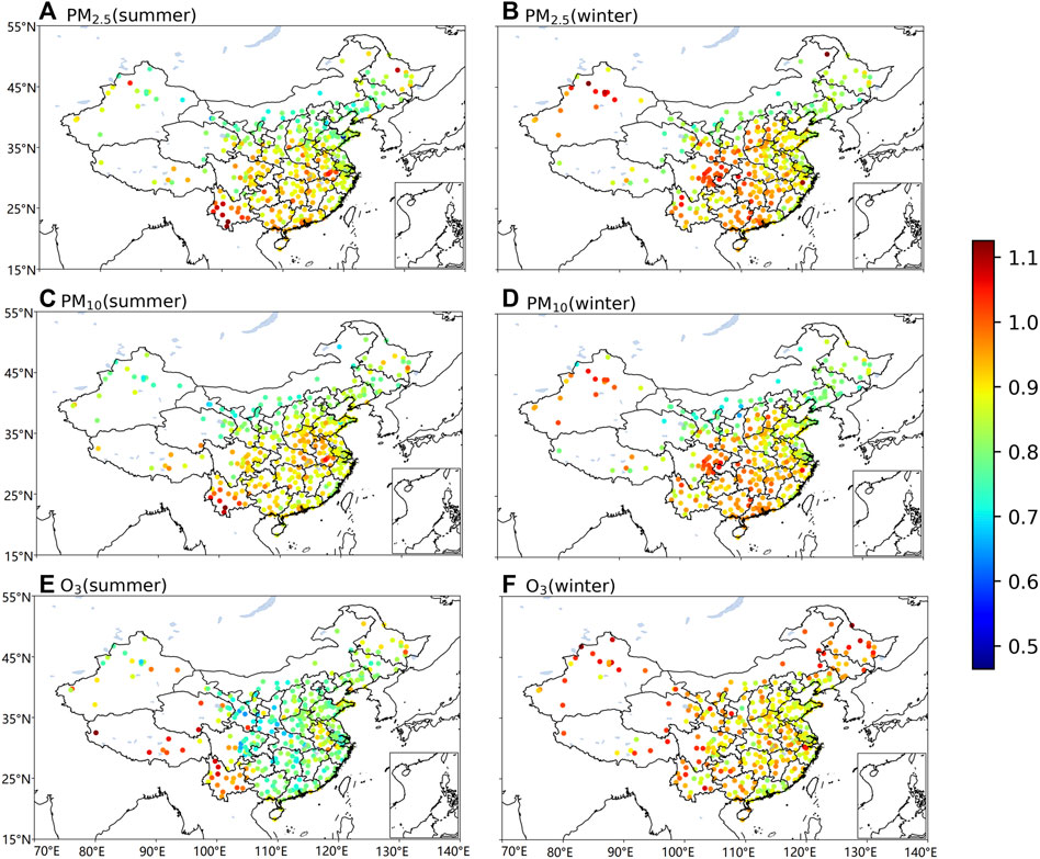
FIGURE 5. (color online) Spatial distributions of the DFA scale exponent $\text{α}$ for (A) PM_2.5, (C) PM₁₀, and (E) O₃ in summer. (B), (D), and (F) are same as (A), (C), and (D) but in winter.

However, the seasonal differences could be affected by the monsoon system. In winter, China is controlled by Siberian high, and the air mass is dry, which is not conducive to precipitation. The atmospheric stratification is relatively stable, and it is easy to accumulate aerosols in the lower atmosphere, which is not conducive to pollutant diffusion. We find that the $\text{α}$ values significantly increase in Eastern and Northern China for O₃ in Figure 5F. It indicates that there is a strong long-term memory for winter there in contrast to PM_2.5 and PM₁₀. It is well known that O₃ is a photochemical oxidant formed by a series of photochemical reactions of nitrogen oxides and volatile organic compounds in the atmosphere [51]. There are more sunny days in winter of Eastern and Northern China. We find that some places, e.g., Sichuan Basin with the short-term memory in Figure 2 also are associated with the long-term memory in Figure 5 in winter. We calculate the spatial correlation coefficient between short (Figure 2) and -term memory (Figure 5) for China, and find that the coefficients are 0.273, 0.226, and 0.164 in summer and 0.303, 0.319, and 0.041 in winter for PM_2.5, PM₁₀, and O₃ respectively. There are more similarities in space between the short- and long-term memory in winter than that of summer for PM_2.5 and PM₁₀. For O₃, the short- and long-term memory are very different and the spatial correlation coefficients are smallest.

Discussions and Conclusion

In this study, we use the AR (1) process and the DFA method to quantify the memory characteristics of the time series of three air pollutants (PM_2.5, PM₁₀, O₃) in China. According to the AR (1) process, we obtain the spatial distribution of the autoregressive parameter a of 366 Chinese cities for summer and winter respectively which is associated with the short-term memory behavior. The short-term memory of particulate matter in most parts of southern China is stronger, especially in the Yangtze River Basin, while the short-term memory of O₃ is slightly different between the north and the south. Moreover, the short-term memory of PM_2.5 and PM₁₀ in winter are stronger than in summer related to the stronger short-term and local meteorological field. In the previous studies [31, 32], they found two different scaling exponents of DFA in short- and long-term scales for PM₁₀ in Shanghai in consistent with us. However, our results suggest that using the scaling exponent of DFA in short-term scale to quantify memory is problematic, since the DFA index can by strongly affected by the limited length of time series [46, 47]. Thus, it is better to use the autoregressive parameter of the AR (1) process.

To quantify the long-term memory behavior, we study the DFA index of different pollutants in Beijing, Shanghai, Chengdu and Guangzhou in winter and summer. We find that the three pollutants in four representative cities have strong long-term memory (the DFA index $\alpha$ greater than 0.5). In comparison to previous studies on the memory analysis of some regions or cities in China [31, 32, 36, 37], our results show the similar long-term memory behaviors. Furthermore, our results suggest that the long-term memory behaviors strongly depend on seasons and locations in China, which are lost in previous studies. To show the spatial pattern of long-term memory in China, we further analyzed the DFA index of pollutant time series in 366 cities across China in summer and winter. It is found that the long-term memory of air pollutants in southern cities is generally higher than those of northern cities for PM pollutions. The long-term memory of O₃ does not show significant differences between southern and northern. The spatial differences of long-term memory of PM pollutions are mainly related to different long-term meteorological conditions in Southern and Northern China. Also, the long-term memory measures of air pollutants in Chinese cities are higher in winter than in summer associated with the longer persistent weather system in winter. There are some spatial similarities between the short- and long-term memory measures for PM_2.5 and PM₁₀. But for O₃, the spatial similarity is very low and irregular. In our further work, we will consider relationships of the memory between air pollution and meteorological factors or human activities from the perspective of dynamic characteristics.

Data Availability Statement

The original contributions presented in the study are included in the article/Supplementary Material, further inquiries can be directed to the corresponding author.

Author Contributions

YZ designed research; PY performed research; PY, YZ and DN analyzed data; PY, WL, YZ and PQ wrote the paper. PY, PQ, DN, WL and YZ contributed to reviewing the manuscript. All authors have read and approved the final manuscript.

Funding

This work was supported by the National Natural Science Foundation of China (No. 61573173).

Conflict of Interest

The authors declare that the research was conducted in the absence of any commercial or financial relationships that could be construed as a potential conflict of interest.

Publisher’s Note

All claims expressed in this article are solely those of the authors and do not necessarily represent those of their affiliated organizations, or those of the publisher, the editors and the reviewers. Any product that may be evaluated in this article, or claim that may be made by its manufacturer, is not guaranteed or endorsed by the publisher.

Acknowledgments

We are grateful for the data resources provided by https://quotsoft.net/air/.

References

1. Tong R, Wang Y, Zhao X, Ma X, Yang X. Comprehensive Comparative Analysis of Air Pollutants Exposure in Different Regions of mainland China: Assessment of Health Impacts and Economic burden. Atmos Pollut Res (2021) 12(10):101210. doi:10.1016/j.apr.2021.101210

CrossRef Full Text | Google Scholar

2. Song J, Wang B, Yang W, Duan H, Liu X. Extracting Critical Supply Chains Driving Air Pollution in China. J Clean Prod (2020) 276:124282. doi:10.1016/j.jclepro.2020.124282

CrossRef Full Text | Google Scholar

3. Liu H, Fang C, Zhang X, Wang Z, Bao C, Li F. The Effect of Natural and Anthropogenic Factors on Haze Pollution in Chinese Cities: a Spatial Econometrics Approach. J Clean Prod (2017) 165:323–33. doi:10.1016/j.jclepro.2017.07.127

CrossRef Full Text | Google Scholar

4. Zhang Z, Zhang X, Gong D, Quan W, Zhao X, Ma Z, et al. Evolution of Surface O3 and PM2.5 Concentrations and Their Relationships with Meteorological Conditions over the Last Decade in Beijing. Atmos Environ (2015) 108:67–75. doi:10.1016/j.atmosenv.2015.02.071

CrossRef Full Text | Google Scholar

5. Zhang Q, Zheng Y, Tong D, Shao M, Wang S, Zhang Y, et al. Drivers of Improved PM 2.5 Air Quality in China from 2013 to 2017. Proc Natl Acad Sci U.S.A (2019) 116:24463–9. doi:10.1073/pnas.1907956116

PubMed Abstract | CrossRef Full Text | Google Scholar

6. Shao M, Wang W, Yuan B, Parrish DD, Li X, Lu K, et al. Quantifying the Role of PM2.5 Dropping in Variations of Ground-Level Ozone: Intercomparison between Beijing and Los Angeles. Sci. Total Environ. (2021) 788(20):147712. doi:10.1016/j.scitotenv.2021.147712

PubMed Abstract | CrossRef Full Text | Google Scholar

7. Song Y, Zhang Y, Wang T, Qian S, Wang S. Spatio-temporal Differentiation in the Incidence of Influenza and its Relationship with Air Pollution in China from 2004 to 2017. Chin Geogr Sci (2021) 31(5):815–28. doi:10.1007/s11769-021-1228-2

PubMed Abstract | CrossRef Full Text | Google Scholar

8. Zhang Y, Zhou D, Fan J, Marzocchi W, Ashkenazy Y, Havlin S. Improved Earthquake Aftershocks Forecasting Model Based on Long-Term Memory. New J Phys (2021) 23:042001. doi:10.1088/1367-2630/abeb46

CrossRef Full Text | Google Scholar

9. Zhang Y, Fan J, Marzocchi W, Shapira A, Hofstetter R, Havlin S, et al. Scaling Laws in Earthquake Memory for Interevent Times and Distances. Phys Rev Res (2020) 2:013264. doi:10.1103/PhysRevResearch.2.013264

CrossRef Full Text | Google Scholar

10. Nian D, Yuan N, Ying K, Liu G, Fu Z, Qi Y, et al. Identifying the Sources of Seasonal Predictability Based on Climate Memory Analysis and Variance Decomposition. Clim Dyn (2020) 55(11):3239–52. doi:10.1007/s00382-020-05444-7

CrossRef Full Text | Google Scholar

11. Franzke CLE, Barbosa S, Blender R, Fredriksen HB, Laepple T, Lambert F, et al. The Structure of Climate Variability across Scales. Rev Geophys (2020) 58(2):e2019RG000657. doi:10.1029/2019RG000657

CrossRef Full Text | Google Scholar

12. Yuan N, Ding M, Ludescher J, Bunde A. Increase of the Antarctic Sea Ice Extent Is Highly Significant Only in the Ross Sea. Sci Rep (2017) 7:41096. doi:10.1038/srep41096

PubMed Abstract | CrossRef Full Text | Google Scholar

13. Peng C-K, Buldyrev SV, Havlin S, Simons M, Stanley HE, Goldberger AL. Mosaic Organization of DNA Nucleotides. Phys Rev E (1994) 49(2):1685–9. doi:10.1103/physreve.49.1685

CrossRef Full Text | Google Scholar

14. Potter KW. Annual Precipitation in the Northeast United States: Long Memory, Short Memory, or No Memory? Water Resour Res (1979) 15(2):340–6. doi:10.1029/WR015i002p00340

CrossRef Full Text | Google Scholar

15. Yuan N, Fu Z, Mao J. Different Scaling Behaviors in Daily Temperature Records over China. Physica A: Stat Mech its Appl (2010) 389(19):4087–95. doi:10.1016/j.physa.2010.05.026

CrossRef Full Text | Google Scholar

16. Talkner P, Weber RO. Power Spectrum and Detrended Fluctuation Analysis: Application to Daily Temperatures. Phys Rev E (2000) 62(1):150–60. doi:10.1103/PhysRevE.62.150

CrossRef Full Text | Google Scholar

17. Costa RL, Vasconcelos GL. Long-range Correlations and Nonstationarity in the Brazilian Stock Market. Physica A (2003) 329(1):231–48. doi:10.1016/S0378-4371(03)00607-1

CrossRef Full Text | Google Scholar

18. Lin G, Chen X, Fu Z. Temporal-spatial Diversities of Long-Range Correlation for Relative Humidity over China. Physica A: Stat Mech Appl (2007) 383(2):585–94. doi:10.1016/j.physa.2007.04.059

CrossRef Full Text | Google Scholar

19. Govindan RB, Vjushin D, Brenner S, Bunde A, Havlin S, Schellnhuber HJ. Long-range Correlations and Trends in Global Climate Models: Comparison with Real Data. Physica A (2001) 294(1-2):239–48. doi:10.1016/S0378-4371(01)00110-8

CrossRef Full Text | Google Scholar

20. Kantelhardt JW, Koscielny-Bunde E, Rego HHA, Havlin S, Bunde A. Detecting Long-Range Correlations with Detrended Fluctuation Analysis. Physica A (2001) 295(3):441–54. doi:10.1016/S0378-4371(01)00144-3

CrossRef Full Text | Google Scholar

21. Auno S, Lauronen L, Wilenius J, Peltola M, Vanhatalo S, Palva JM. Detrended Fluctuation Analysis in the Presurgical Evaluation of Parietal Lobe Epilepsy Patients. Clin Neurophysiol (2021) 132(7):1515–25. doi:10.1016/j.clinph.2021.03.041

PubMed Abstract | CrossRef Full Text | Google Scholar

22. Sanyal MK, Ghosh I, Jana RK. Characterization and Predictive Analysis of Volatile Financial Markets Using Detrended Fluctuation Analysis, Wavelet Decomposition, and Machine Learning. IJDA (2021) 2(1):1–31. doi:10.4018/IJDA.2021010101

CrossRef Full Text | Google Scholar

23. Fan J, Zhou D, Shekhtman LM, Shapira A, Hofstetter R, Marzocchi W, et al. Possible Origin of Memory in Earthquakes: Real Catalogs and an Epidemic-type Aftershock Sequence Model. Phys Rev E (2019) 99(4-1):042210. doi:10.1103/PhysRevE.99.042210

PubMed Abstract | CrossRef Full Text | Google Scholar

24. Lachowycz SM, Pyle DM, Mather TA, Varley NR, Odbert HM, Cole PD, et al. Long-range Correlations Identified in Time-Series of Volcano Seismicity during Dome-Forming Eruptions Using Detrended Fluctuation Analysis. J Volcanol Geothermal Res (2013) 264:197–209. doi:10.1016/j.jvolgeores.2013.07.009

CrossRef Full Text | Google Scholar

25. Lennartz S, Livina VN, Bunde A, Havlin S. Long-term Memory in Earthquakes and the Distribution of Interoccurrence Times. Europhys Lett (2008) 81(6):69001. doi:10.1209/0295-5075/81/69001

CrossRef Full Text | Google Scholar

26. Yang L, Fu Z. Process-dependent Persistence in Precipitation Records. Physica A: Stat Mech Appl (2019) 527:121459. doi:10.1016/j.physa.2019.121459

CrossRef Full Text | Google Scholar

27. Yuan N, Ding M, Huang Y, Fu Z, Xoplaki E, Luterbacher J. On the Long-Term Climate Memory in the Surface Air Temperature Records over Antarctica: A Nonnegligible Factor for Trend Evaluation. J Clim (2015) 28(15):5922–34. doi:10.1175/JCLI-D-14-00733.1

CrossRef Full Text | Google Scholar

28. Zhang Y, Chen D, Fan J, Havlin S, Chen X. Correlation and Scaling Behaviors of fine Particulate Matter (PM 2.5 ) Concentration in China. EPL (2018) 122(5):58003. doi:10.1209/0295-5075/122/58003

CrossRef Full Text | Google Scholar

29. Lin W, Xu X, Ma Z, Zhao H, Liu X, Wang Y. Characteristics and Recent Trends of Sulfur Dioxide at Urban, Rural, and Background Sites in North China: Effectiveness of Control Measures. J Environ Sci (2012) 24(1):34–49. doi:10.1016/S1001-0742(11)60727-4

CrossRef Full Text | Google Scholar

30. Mouzourides P, Kyprianou A, Neophytou MK-A. Exploring the Multi-Fractal Nature of the Air Flow and Pollutant Dispersion in a Turbulent Urban Atmosphere and its Implications for Long Range Pollutant Transport. Chaos (2021) 31(1):013110. doi:10.1063/1.5123918

PubMed Abstract | CrossRef Full Text | Google Scholar

31. Liu Z, Wang L, Zhu H. A Time-Scaling Property of Air Pollution Indices: a Case Study of Shanghai, China. Atmos Pollut Res (2015) 6(5):886–92. doi:10.5094/APR.2015.098

CrossRef Full Text | Google Scholar

32. Kai S, Chun-qiong L, Nan-shan A, Xiao-hong Z. Using Three Methods to Investigate Time-Scaling Properties in Air Pollution Indexes Time Series. Nonlinear Anal Real World Appl (2008) 9(2):693–707. doi:10.1016/j.nonrwa.2007.06.003

CrossRef Full Text | Google Scholar

33. Nikolopoulos D, Moustris K, Petraki E, Cantzos D. Long-memory Traces in $$\hbox {PM}_{10}$$ Time Series in Athens, Greece: Investigation through DFA and R/S Analysis. Meteorol Atmos Phys (2021) 133(2):261–79. doi:10.1007/s00703-020-00744-3

CrossRef Full Text | Google Scholar

34. Windsor HL, Toumi R. Scaling and Persistence of UK Pollution. Atmos Environ (2001) 35(27):4545–56. doi:10.1016/S1352-2310(01)00208-4

CrossRef Full Text | Google Scholar

35. Plocoste T, Calif R, Jacoby-Koaly S. Temporal Multiscaling Characteristics of Particulate Matter PM10 and Ground-Level Ozone O3 Concentrations in Caribbean Region. Atmos Environ (2017) 169:22–35. doi:10.1016/j.atmosenv.2017.08.068

CrossRef Full Text | Google Scholar

36. Wu B, Liu CQ, Zhang J, Li YH, Chen YB, Wen Y, et al. Nonlinear Dynamic Mechanism of Regional Air Pollution during the COVID-19 Lockdown. China Environ.Sci (2021) 41(5):2028–39. doi:10.19674/j.cnki.issn1000-6923.2021.0213

CrossRef Full Text | Google Scholar

37. Wu SH, Shi K, Liu CQ, Li SC, Huang Y, Yin H. Long-term Persistence Characteristics of PM_2.5 Evolution during a Typical Haze Episode in Chengdu. Environ Sci Technol (2014) 37(10):9–14. doi:10.3969/j.issn.1003-6504.2014.10.002

CrossRef Full Text | Google Scholar

38. Chen BW, Xia L. Research on Parameter Estimation of AR(p) Model Based on Approximate Bayesian Computation. Adv Appl Math (2021) 10(3):680–8. doi:10.12677/AAM.2021.103074

CrossRef Full Text | Google Scholar

39. Peng CK, Hausdorff JM, Havlin S, Mietus JE, Stanley HE, Goldberger AL. Multiple-time Scales Analysis of Physiological Time Series under Neural Control. Physica A (1998) 249(1):491–500. doi:10.1016/s0378-4371(97)00508-6

PubMed Abstract | CrossRef Full Text | Google Scholar

40. Tai APK, Mickley LJ, Jacob DJ. Correlations between fine Particulate Matter (PM2.5) and Meteorological Variables in the United States: Implications for the Sensitivity of PM2.5 to Climate Change. Atmos Environ (2010) 44(32):3976–84. doi:10.1016/j.atmosenv.2010.06.060

CrossRef Full Text | Google Scholar

41. Li L, Qian J, Ou C-Q, Zhou Y-X, Guo C, Guo Y. Spatial and Temporal Analysis of Air Pollution Index and its Timescale-dependent Relationship with Meteorological Factors in Guangzhou, China, 2001-2011. Environ Pollut (2014) 190:75–81. doi:10.1016/j.envpol.2014.03.020

PubMed Abstract | CrossRef Full Text | Google Scholar

42. Yang X, Wang S, Zhang W, Zhan D, Li J. The Impact of Anthropogenic Emissions and Meteorological Conditions on the Spatial Variation of Ambient SO2 Concentrations: A Panel Study of 113 Chinese Cities. Sci Total Environ (2017) 584-585:318–28. doi:10.1016/j.scitotenv.2016.12.145

PubMed Abstract | CrossRef Full Text | Google Scholar

43. Zhang Y, Fan J, Chen X, Ashkenazy Y, Havlin S. Significant Impact of Rossby Waves on Air Pollution Detected by Network Analysis. Geophys Res Lett (2019) 46(21):12476–85. doi:10.1029/2019GL084649

CrossRef Full Text | Google Scholar

44. Huang Y, Fu Z. Enhanced Time Series Predictability with Well-Defined Structures. Theor Appl Climatol (2019) 138:373–85. doi:10.1007/s00704-019-02836-6

CrossRef Full Text | Google Scholar

45. Fu S, Huang Y, Feng T, Nian D, Fu Z. Regional Contrasting DTR's Predictability over China. Physica A: Stat Mech Appl (2019) 521(1):282–92. doi:10.1016/j.physa.2019.01.077

CrossRef Full Text | Google Scholar

46. Höll M, Kantz H. The Fluctuation Function of the Detrended Fluctuation Analysis - Investigation on the AR(1) Process. Eur Phys J B (2015) 88(5):1–9. doi:10.1140/epjb/e2015-60143-1

CrossRef Full Text | Google Scholar

47. Maraun D, Rust HW, Timmer J. Tempting Long-Memory - on the Interpretation of DFA Results. Nonlin Process. Geophys (2004) 11:495–503. doi:10.5194/npg-11-495-2004

CrossRef Full Text | Google Scholar

48. Zhao Z, Xi H, Russo A, Du H, Gong Y, Xiang J, et al. The Influence of Multi-Scale Atmospheric Circulation on Severe Haze Events in Autumn and Winter in Shanghai, China. Sustainability (2019) 11(21):5979. doi:10.3390/su11215979

CrossRef Full Text | Google Scholar

49. Leung DM, Tai APK, Mickley LJ, Moch JM, van Donkelaar A, Shen L, et al. Synoptic Meteorological Modes of Variability for fine Particulate Matter (PM2.5) Air Quality in Major Metropolitan Regions of China. Atmos Chem Phys (2018) 18:6733–48. doi:10.5194/acp-18-6733-2018

CrossRef Full Text | Google Scholar

50. Wise E, Comrie A. Meteorologically Adjusted Urban Air Quality Trends in the Southwestern United States. Atmos Environ (2005) 39(16):2969–80. doi:10.1016/j.atmosenv.2005.01.024

CrossRef Full Text | Google Scholar

51. Liu C, Shi K. A Review on Methodology in O3-NOx-VOC Sensitivity Study. Environ Pollut (2021) 291:118249. doi:10.1016/j.envpol.2021.118249

PubMed Abstract | CrossRef Full Text | Google Scholar