The Spillover Effect and Dynamic Correlation of the China-US Bean Futures Markets Based on Investor Sentiment

This study analyzes the spillover effect and dynamic correlation of the China-US bean futures markets and discusses the relationship between the dynamic correlation of the bean futures price index and investor sentiment. First, the spillover effect of the China-US bean futures markets is analyzed through the BEKK-GARCH model. Then, the DCC-GARCH model is used for obtaining the dynamic correlation coefficients of the China-US bean futures markets. Next, the principal component analysis method is chosen to construct a comprehensive investor sentiment index. Lastly, the dynamic impacts between the change in investor sentiment and the correlation of the China-US bean futures price index are discussed through the ensemble empirical mode decomposition and impulse response analysis. The results show that the spillover effect of different degrees and directions exists between the China-US bean futures markets, and the dynamic correlation coefficients among different bean futures are also different. Besides, a certain degree of interactions exists between the high-frequency and low-frequency components of the comprehensive investor sentiment index and the dynamic correlations of bean futures price indexes.

Introduction

As the earliest commodity futures markets, agricultural futures markets play an essential role in risk aversion and price discovery [1, 2]. In 1993, the Chinese soybean futures trading variety “yellow soybean” was listed in the Dalian Commodity Exchange (abbreviated as DCE). Besides, DCE launched soybean oil futures in 2000 and soybean meal futures in 2006. At present, DCE has gradually formed an integrity and maturity bean futures market [3, 4]. The United States, as the leading producer in international soybean markets, is China’s largest cooperative partner of soybean products [5]. In such circumstances, the American soybean futures market greatly influences the Chinese bean futures market [6]. The Chicago Board of Trade in the United States (abbreviated as CBOT) is a leading agricultural futures exchange globally. Thus, this paper comparatively analyzes the price fluctuation of bean futures in DCE and CBOT to discuss the spillover effect and the dynamic correlation of the bean futures market in China and the US.

In the existing literature, most studies on the price linkage and the spillover effect of bean futures prices could be summed up as two parts: the research based on spatial perspective and futures variety perspective. The spatial perspective emphasized the price linkage effect and the spillover effect of bean futures prices between different areas or countries [2, 7–9]. For example, a transmission relationship of soybean prices could be seen from the Chicago Board of Trade (CBOT) to the Rotterdam soybean market, the Brazilian soybean market, and the Argentine soybean market [10]. Besides, a multivariate generalized autoregressive conditional heteroskedasticity model was used for analyzing a two-way spillover relationship between copper and soybean futures markets in Chinese and the US markets [11]. The results showed that the two-way spillover effect was stronger in the US markets. Under the circumstance of Sino-US trade friction in 2018, the DMCA and MFDMA methods were used for analyzing the multifractality features of soybean futures markets in China and the US [12]. It concluded that the cross-correlations coefficients decreased significantly during the Sino-US trade friction. As for the futures variety perspective, some scholars emphatically discussed the price linkage effect and the spillover effect between different grain crops and soybeans or between energy products and soybeans [13–16]. For example, Liu et al. constructed a model based on Markov-switching GRG copula to analyze the dependence structure between the WTI (BRENT) crude oil futures price and the futures price of Chinese agricultural commodity, and verified the existence of two structural states of Markov switching [17]. A long-term co-integration relationship was found between the price of agricultural products and world crude oil. For a long time, the soybean oil price greatly influenced the edible oil market, but the impact of crude oil prices on edible oil prices was not significant during the sample period [18]. And Zhang et al. again confirmed no long-term relationship between fuel prices and agricultural product prices [19]. Based on the VARMA-BEKK-GARCH model, Han et al. found an increasingly evident two-way fluctuation linkage between energy prices and agricultural futures returns under the influence of external shocks [20]. After analyzing the link between US soybean prices and the Dow Jones U.S. Water Index (DJUSWU), Jiang and Fortenbery found that the El Niño event significantly strengthened the link between soybeans and the water property market [21]. The above research mainly involves the price linkage and the spillover effect between soybean and other commodity markets. For international commodities markets, the changes in commodity prices can directly affect international trade and international capital flows, thereby affecting the development of the world economy. Taxonomy of commodities assets based on the complexity-entropy causality plane is also an essential component for the research on commodity price fluctuation, whether in the spot market or the futures market [22, 23].

Although much research discussed the spillover effect between agricultural product markets, the existing studies mainly have several shortcomings.

1) First, the existing studies lack attention to soybean oil and soybean meal futures that are increasingly important in the international and domestic markets.

2) Second, the existing studies focus on studying the spillover effect between soybean futures and neglect the dynamic correlation of the China-US bean futures markets.

3) Third, the existing studies don’t consider the high-frequency component and low-frequency component of the comprehensive investor sentiment index in the study process.

Based on the shortcomings of the existing studies, the contributions of this paper are in the following three aspects.

1) First, this paper discusses the spillover effect of soybean futures markets, soybean meal futures markets, and soybean oil futures markets from the perspective of investor sentiment. As the research content contains soybean meal futures markets and soybean oil futures markets relative to existing literature, the conclusions can reflect the spillover effect and dynamic correlation of the China-US bean futures markets more realistically.

2) Second, this paper analyzes the spillover effect between the China-US bean futures markets and the dynamic correlation of the China-US bean futures markets.

3) Third, this paper studies the relationship between the dynamic correlation of the China-US bean futures markets and the high-frequency and low-frequency components of the comprehensive investor sentiment index.

Data Description

This section gives details of the sample selection, the input variables for the model prediction, and the data resources. Specifically, the daily closing prices are selected in DCE and CBOT to analyze the spillover effect and the dynamic correlation of the China-US bean futures markets. In DCE, soybean oil futures were listed in January 2006. And in CBOT, soybean oil futures and soybean meal futures were recorded in 2013. After sorting out sample data at different time intervals, the daily data of bean futures are chosen 1812 from January 4, 2013, to January 3, 2020, in DCE and CBOT.

For the seek of constructing the daily investor sentiment comprehensive index, trading volume (VOL) and psychological linear index (PSY) are used as proxy variables of investor sentiment [24, 25]. And the position holding and trading volume are usually used for constructing the investor sentiment index [26]. A comprehensive investor sentiment index is built based on the psychological linear index (PSY), the position factor (OPENI), the volume factor (VOLI), and the current price difference (GAP). The calculation method of each indicator is as follows.

$\text{PSY}=\frac{T_u}{T}\times 100(1)$

In expression (1), T_u represents the number of days that the log price index on day t is higher than the log price index on day t-1, and T indicates the trading period.

${\text{OPENI}}_t=\frac{OPE{N}_t-\text{min}\left(OPE{N}_t\right)}{\max \left(OPE{N}_t\right)-\text{min}\left(OPE{N}_t\right)}(2)$

In expression (2), OPENI_t shows the position factor on day t. It indicates the position volume on day t.

${\text{VOLI}}_t=\frac{{\text{VOL}}_t-\text{min}\left({\text{VOL}}_t\right)}{\max \left({\text{VOL}}_t\right)-\text{min}\left({\text{VOL}}_t\right)}(3)$

Similarly, VOLI_t shows the volume factor on day t in expression (3). It indicates the trading volume on day t.

${\text{GAP}}_t=future\_pric{e}_t-spot\_pric{e}_t(4)$

Besides, future_price_t shows the futures price on day t, and spot_price_t represents the spot price on day t in expression (4).

Figure 1 shows the return yield series of bean futures in DCE and CBOT. The above return yield series of futures price indexes are called logarithmic yield and expressed as R_dd, R_dp, R_dy, R_cd, R_cp, and R_cy, in turn. It can be seen from Table 1 that the skewness of R_dy and R_cy is greater than zero, showing a right-skewed distribution. Conversely, other return yield series show a left-skewed distribution. The kurtosis is greater than zero for R_dd, R_cd, and R_cp, indicating a sharp peak and trailing tail distribution. And for R_dp, R_dy, and R_cy, the kurtosis is less than zero, showing a thin-tailed distribution. Besides, all JB-statistics of return yield series in Table 1 are much larger than 5.99, the critical value at the 5% significant level. It means that they do not follow the standard normal distribution. And the ADF and PP test presents that these series are non-stationary. Therefore, the first-order difference should be carried out before the GARCH model is built.

FIGURE 1

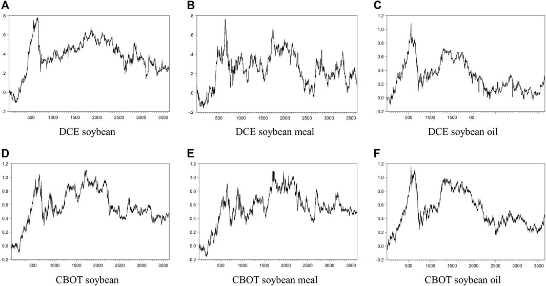
FIGURE 1. The evolutionary temporal of daily return yield series of bean futures from January 4, 2013, to January 3, 2020. (A–C) show the evolutionary temporal of daily return yield series in DCE, and (D–F) show the evolutionary temporal of daily return yield series in CBOT.

TABLE 1

TABLE 1. The descriptive statistics of bean price series.

Models

BEKK-GARCH Model

The BEKK-GARCH model, first proposed by Engle and Kroner, is one of the multivariable GARCH models [27]. It can effectively ensure the positive definiteness of the covariance matrix under weak conditions [28]. The BEKK-GARCH model has a higher forecasting ability than other GARCH models [29]. For the multivariate BEKK-GARCH model, the asymptotic properties of the variance-targeting estimator can be further discussed by the multivariate BEKK model based on variance targeting [30]. Besides, Markov regime-switching framework is also used in a BEKK-GARCH model to study hedge performance in the financial market [31]. If the conditional variance follows the GARCH (1, l) process, the variance equation of binary BEKK is expressed as follows.

${\text{H}}_t=C{C}^T+A\left({\epsilon }_{t-1}{\epsilon }_{t-1}^T\right)A^T+B{H}_{t-1}{B}^T(5)$

$H_t=\left|\begin{array}{cc}{h}_{11,t}& h_{12,t}\\ h_{21,t}& h_{22,t}\end{array}\right|(6)$

$C_t=\left|\begin{array}{cc}{c}_{11,t}& 0\\ c_{21,t}& c_{22,t}\end{array}\right|(7)$

$A_t=\left|\begin{array}{cc}{a}_{11,t}& a_{12,t}\\ a_{21,t}& a_{22,t}\end{array}\right|(8)$

$B_t=\left|\begin{array}{cc}{b}_{11,t}& b_{12,t}\\ b_{21,t}& b_{22,t}\end{array}\right|(9)$

In expression (5), H_t is a 2 × 2 dimensional matrix representing the first-order variance-covariance matrix of the conditional residual within time t. C is a constant upper triangular matrix. The main diagonal elements in A and B are the coefficients of ARCH and GARCH terms, respectively. After expanding the above expressions, each element of the conditional variance-covariance matrix can be written as follows.

$h_{11,t}=c_{11}^2+b_{11}^2{h}_{11,t-1}+2b_{11}{b}_{21}{h}_{12,t-1}+b_{21}^2{h}_{22,t-1}+a_{11}^2{\epsilon }_{1,t-1}^2+2a_{11}{a}_{21}{\epsilon }_{1,t-1}{\epsilon }_{2,t-1}+a_{21}^2{\epsilon }_{2,t-1}^2(10)$

$h_{22,t}=\left(c_{11}^2+c_{22}^2\right)+b_{12}^2{h}_{11,t-1}+2b_{12}{b}_{22}{h}_{12,t-1}+b_{22}^2{h}_{22,t-1}+a_{12}^2{\epsilon }_{1,t-1}^2+2a_{22}{a}_{12}{\epsilon }_{1,t-1}{\epsilon }_{2,t-1}+a_{22}^2{\epsilon }_{2,t-1}^2(11)$

$h_{12,t}=h_{21,t}=c_{11}{c}_{21}+b_{11}{b}_{12}{h}_{11,t-1}+\left(b_{11}{b}_{22}+b_{21}{b}_{12}\right)h_{12,t-1}+b_{21}{b}_{22}{h}_{22,t-1}+a_{11}{a}_{12}{\epsilon }_{1,t-1}^2+\left(a_{11}{a}_{22}+a_{12}{a}_{21}\right){\epsilon }_{1,t-1}{\epsilon }_{2,t-1}+a_{22}{a}_{21}{\epsilon }_{2,t-1}^2(12)$

In expressions (10), (11) and (12), h_11,t is the conditional variance in DCE; h_22,t is the conditional variance in CBOT; h_12,t is the conditional covariance between DCE and CBOT.

The spillover effect of time series in one futures market is divided into volatility clustering and volatility persistence. The main diagonal elements a₁₁ and a₂₂ in matrix A represent the volatility clustering of the futures market, known as the ARCH-type spillover effect. The main diagonal elements b₁₁ and b₂₂ in matrix B represent the volatility persistence of the futures market, known as the GARCH-type spillover effect.

The spillover effect between futures markets includes the shock conduction effect and the volatility conduction effect. The off-diagonal elements in matrix A are named the shock conduction effect. Specifically, a₁₂ expresses the conduction effect from CBOT to DCE, and a₂₁ denotes the conduction effect from DCE to CBOT. Similarly, the off-diagonal elements in matrix B are named the volatility conduction effect. Specifically, b₁₂ shows the volatility conduction effect from CBOT to DCE, and b₂₁ represents the volatility conduction effect from DCE to CBOT.

The Wald test is used to determine the type of spillover effect between the two markets, including one-way overflow and two-way overflow. If the constraints between the two futures markets are valid, the estimated parameter values should follow the original hypothesis under unconstrained conditions. The original hypothesis is summarized in three forms: Hypothesis I, Hypothesis II, and Hypothesis III.

Hypothesis I: There is no mutual spillover effect between the two markets,

$H_0:a_{21}=b_{21}=0; a_{12}=b_{12}=0.(13)$

Hypothesis II: There is no spillover effect from DCE to CBOT (one-way spillover),

$H_0:a_{21}=b_{21}=0.(14)$

Hypothesis III: There is no spillover effect from CBOT to DCE (one-way spillover),

$H_0:a_{12}=b_{12}=0.(15)$

The statistics of the Wald test can be written as follows.

$Z_i=a_i/{\sigma }_a(16)$

$\text{W}=Z_1^2+Z_2^2+\cdots +Z_h^2 \sim {\chi }^2\left(h\right)(17)$

In a Walt test, Z is the column vector, which is comprised of Z_i. And Z_i is the z-statistic value under the ith constraint, h is the number of constraints.

DCC-GARCH Model

The DCC-GARCH model can be used to study the volatility clustering of individual variables and analyze the strength of the relationships between two variables [32]. This model is especially suitable for studying financial contagion between developed and emerging market countries [33]. Besides, it can also be used in macroeconomic studies, such as the time-varying correlation between different macroeconomic factors [34]. It assumes that the return on assets in period t follows a conditional multidimensional normal distribution with zero mean and covariance matrix H_t. The series r_t for t = 1,...,T, is decomposed into conditional expected returns and residuals.

$r_t={\mu }_t+{\sigma }_t(18)$

${\sigma }_t=H_t^{\frac{1}{2}}{\eta }_t(19)$

$H_t=D_t{R}_t{D}_t={\rho }_{i,j,t}\sqrt{h_{ii,t}{h}_{jj,t}}(20)$

$D_t=diag\left(\sqrt{h_{11,t}},\dots ,\sqrt{h_{nn,t}}\right)(21)$

In expressions (20) and (21), $D_t$ contains the conditional variances, and $R_t$ contains the conditional correlations.

$h_{ii,t}^2={\gamma }_i+{\displaystyle \sum _{p=1}^{P_i}{a}_{ip}{\epsilon }_{i,t-p}^2}+{\displaystyle \sum _{q=1}^{Q_i}{\beta }_{ip}{h}_{i,t-q}^2}, i=1,\dots ,n(22)$

In expression (22), ${\epsilon }_t$ is a standardized residual, obtained by the mean equation in the GARCH process. Besides, $a_i$ expresses the coefficient of ARCH term, and ${\beta }_j$ is the coefficient of GARCH term. They satisfy ${\displaystyle \sum _{i=1}^P{a}_i}+{\displaystyle \sum _{j=1}^q{\beta }_j}<1$, and $a_i+{\beta }_j\ge 0$. The conditional correlation matrix $R_t$ is expressed as expression (23).

$R_t=diag{\left(Q_t\right)}^{-\frac{1}{2}}{Q}_{t}diag{\left(Q_t\right)}^{-\frac{1}{2}}(23)$

$Q_t=\overline{Q}+a\left(z_{t-1}{z^{\prime }}_{t-1}-\overline{Q}\right)+b\left(Q_{t-1}-\overline{Q}\right)=\left(1-a-b\right)\overline{Q}+a{z}_{t-1}{z^{\prime }}_{t-1}+b{Q}_{t-1}(24)$

In expression (24), $z_t$ is the standardized error, $Q_t$ is the positive definite matrix, and $\overline{Q}$ is the positive definite unconditional correlation matrix. When a DCC model satisfies a mean regression process, the nonnegative a and b satisfy the constraint $\text{a}+\text{b}<1$.

Therefore, for market i and market j, their dynamic condition correlation coefficient at time t is expressed as expression (25).

${\rho }_{ij}=\frac{q_{ij,t}}{\sqrt{q_{ii,t}\times q_{jj,t}}}=\frac{\left(1-a-b\right)\overline{q_{ij}}+b{q}_{ij,t-1}+a{z}_{i,t-1}{z}_{j,t-1}}{\sqrt{\left[\left(1-a-b\right)\overline{q_{ii}}+a{z}_{i,t-1}^2+b{q}_{ii,t-1}\right]}+\sqrt{[\left(1-a-b\right)\overline{q_{jj}}+a{z}_{j,t-1}^2+b{q}_{jj,t-1}]}}(25)$

Results

The Spillover Effect in the China-US Bean Futures Markets

The ADF test is conducted on the six sets of logarithmic price index series in Table 2, and all p-values are greater than 0.05. It is indicated that all futures price index series are non-stationary series. In order to get stationary sequences, the first-order difference needs to be conducted. After that, we obtain the series and plot the result of the first-order differentiation process in Figure 2, which presents that the return for financial time series is stationary [35].

TABLE 2

TABLE 2. The results of the ADF test.

FIGURE 2

FIGURE 2. The result of the first-order differentiation process.

Table 3 shows the test results of the spillover effect between the China-US bean futures markets based on the multivariate BEKK-GARCH (1,1) model. It can be seen that the four diagonal elements, coming from coefficient matrix A in the ARCH term and coefficient matrix B in the GARCH term of the BEKK-GARCH (1,1) model, have passed the 1% significant level test. It indicates that the fluctuation of the futures price index in one market is subject to the previous fluctuation in this market and another market. Thus, there are significant volatility clustering, volatility persistence, shock conduction effects, and volatility conduction effects in DCE and CBOT.

TABLE 3

TABLE 3. The Estimators of the BEKK-GARCH (1,1) model.

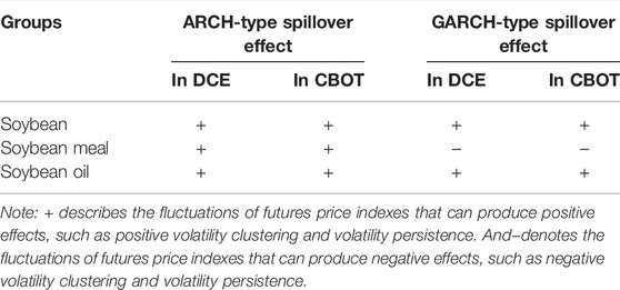
In the BEKK-GARCH model, a₁₁ and a₂₂ represent the ARCH-type spillover effect, and b₁₁ and b₂₂ represent the GARCH-type spillover effect. These two spillover effects are derived from the time series change in one futures market. The details are as follows.

If a₁₁ is greater (or less) than zero, the fluctuation of the futures price index can produce positive (or negative) volatility clustering in DCE.

If a₂₂ is greater (or less) than zero, the fluctuation of the futures price index can produce positive (or negative) volatility clustering in CBOT.

If b₁₁ is greater (or less) than zero, the fluctuation of the futures price index can produce positive (or negative) volatility persistence in DCE.

If b₂₂ is greater (or less) than zero, the fluctuation of the futures price index can produce positive (or negative) volatility persistence in CBOT.

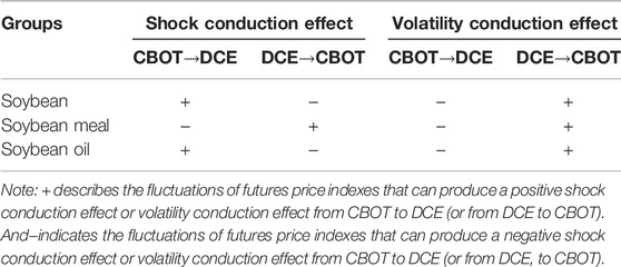
Similarly, a₁₂ and a₂₁ represent the shock conduction effect, and b₁₂ and b₂₁ represent the volatility conduction effect. These two spillover effects are derived from the time series change between DCE and CBOT. The details are as follows.

If a₁₂ is greater (or less) than zero, the fluctuation of the futures price index can produce a positive (or negative) shock conduction effect on the futures price index from CBOT to DCE.

If a₂₁ is greater (or less) than zero, the fluctuation of the futures price index can produce a positive (or negative) shock conduction effect on the futures price index from DCE to CBOT.

If b₁₂ is greater (or less) than zero, the fluctuation of the futures price index can produce a positive (or negative) volatility conduction effect on the futures price index from CBOT to DCE.

If b₂₁ is greater (or less) than zero, the fluctuation of the futures price index can produce a positive (or negative) volatility conduction effect on the futures price index from DCE to CBOT.

The ARCH-type and GARCH-type spillover effects are shown in Table 4, and the shock and volatility conduction effects are shown in Table 5. The symbol + (or –) shows a positive (or negative) effect.

TABLE 4

TABLE 4. The spillover effects deriving from one futures market itself.

TABLE 5

TABLE 5. The spillover effects between DCE and CBOT futures markets.

Table 6 shows the Wald test of parameters estimated by the BEKK-GARCH (1,1) model. The p-value of the test result of the mutual fluctuation spillover effect in the China-US soybean futures markets is less than 5%, reflecting a mutual spillover effect. However, based on the result of the one-way test, the null hypothesis “there is no spillover effect from DCE to CBOT” is rejected at the 10% significant level, and the null hypothesis that “there is no spillover effect from CBOT to DCE” has not been rejected. The three null hypotheses are rejected at the 1% significant level for soybean meal and soybean oil futures markets. The results show that soybean meal and soybean oil futures markets have apparent spillover effects between China and the US.

TABLE 6

TABLE 6. The results of the Wald test.

The Dynamic Correlation of the China-US Bean Futures Markets

The first-order difference sequences of the logarithmic price indexes are used for constructing the optimal ARMA model based on the AIC minimum criterion. The parameters of the optimal ARMA model are shown in Table 7.

TABLE 7

TABLE 7. The parameters of the optimal ARMA model.

The heteroscedasticity test is performed on the residuals of each ARMA model in Figure 3. It is seen that the p-values of ARCH effect tests in six ARMA models are all less than 0.05 after the first order. So, all residual sequences have significant heteroscedasticity.

FIGURE 3

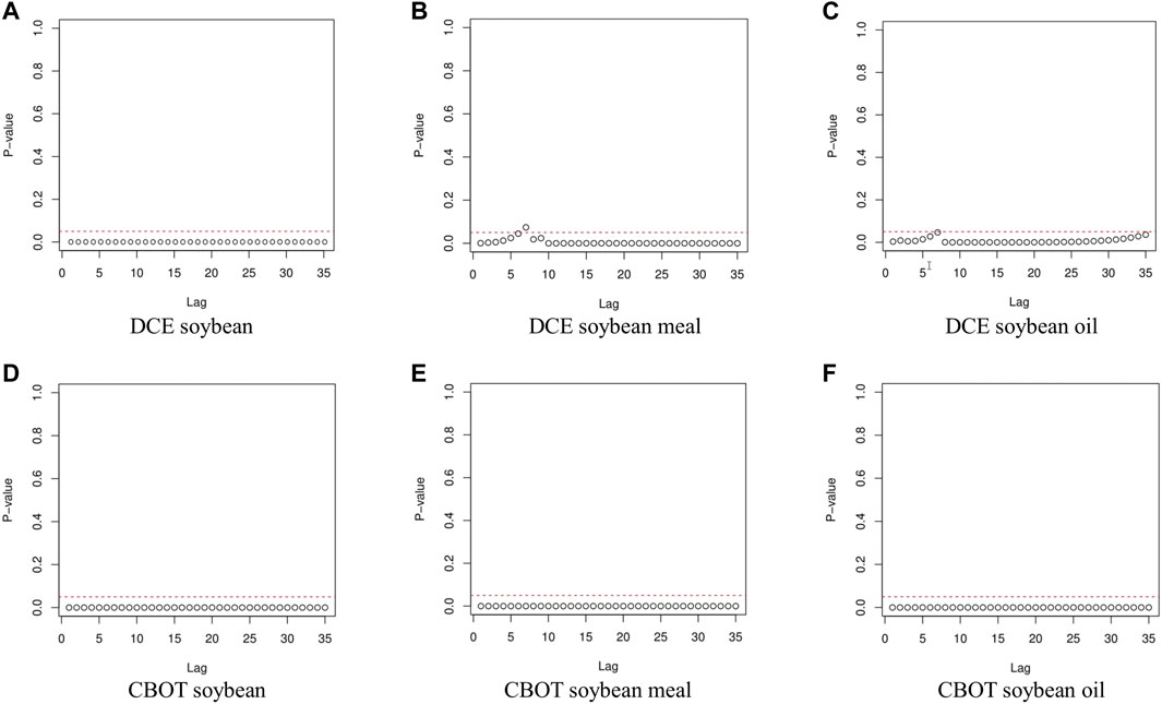
FIGURE 3. The results of the heteroscedasticity test. (A–C) show the results of the heteroscedasticity test in DCE, and (D–F) show the results of the heteroscedasticity test in CBOT.

On this basis, DCC-GARCH models are established to obtain the dynamic correlation coefficients of the China-US bean futures price index. Table 8 shows the parameters estimated by DCC-GARCH models, and Figure 4 shows three sets of dynamic correlation coefficients.

TABLE 8

TABLE 8. The estimated parameters in the DCC-GARCH model.

FIGURE 4

FIGURE 4. The dynamic correlation coefficient of the China-US bean futures markets. (A) shows the dynamic correlation of soybean between the two markets. (B) presents that of soybean meal between the two markets, and (C) presents that of soybean oil between the two markets. For each panel, the horizontal axis represents time, and the vertical axis represents the degree of dynamic correlation.

In Table 8, the sum of a and β of each sequence is less than and close to 1. For soybean futures markets, the value of a₁ is 0.7557. It means that the soybean futures conditional variance in DCE is affected by the square term of the previous residual. In CBOT, the value of β₂ is 0.9381, showing that the volatility of the soybean futures series in CBOT is persistent.

For soybean meal futures markets, the values of a₁ and a₂ are 0.0229 and 0.0622, indicating that the square term of the residual in the previous period has a small influence on the conditional variance of the soybean meal futures series in DCE and CBOT, respectively. And the values of β₁ and β₂ are 0.9761 and 0.9259, reflecting that the volatility of soybean meal futures series has significant persistence in DCE and CBOT. The value of b equals 0.908639, reflecting that the dynamic correlation of soybean meal futures between DCE and CBOT has a long-term effect in time aspect.

For soybean oil futures markets, the value of a₂ is 0.0351, indicating that the conditional variance of soybean oil futures in CBOT is affected by the square term of the previous residual to a lower degree. The value of β₂ equals 0.9570, showing that the soybean oil futures series in CBOT have persistent volatility. In addition, the value of a is 0.0050, reflecting that the dynamic correlation coefficient is less affected by the previous product of standardized residuals. And the value of b is 0.9894, showing that the dynamic correlation of soybean meal futures between DCE and CBOT has a long-term effect in time.

It is seen in Figure 4 that the dynamic correlation coefficients of the China-US soybean and soybean meal futures markets are relatively stable during the sample period. But, the dynamic correlation coefficient greatly fluctuates in the China-US soybean oil futures market.

The Construction of Investor Sentiment Composite Index

Psychological linear index (PSY), position factor (OPENI), volume factor (VOLI), and current price difference (GAP) are chosen as the source indicators to construct a comprehensive investor sentiment index. In Table 9, the p-values of six groups in the 1^st Bartlett spherical test are all less than 0.01. It means the conditions of the principal component analysis are met.

TABLE 9

TABLE 9. The results of the 1st Bartlett spherical test.

The results of the principal component analysis are shown in Table 10. As the cumulative variance explanation rate of the first four principal components exceeds 90%, the first four principal components are weighted to get the initial investor sentiment index (ISI).

TABLE 10

TABLE 10. The cumulative variance explanation rate.

Table 11 shows the correlation coefficients between initial investor sentiment indexes and eight indicators. For each investor sentiment index in Table 11, the correlation between source indicator sequence and ISI almost equals that between the one-period lag value sequence of source indicator sequence and ISI.

TABLE 11

TABLE 11. The correlation coefficients between initial investor sentiment indexes and eight indicators.

In order to verify the feasibility of this analysis method, the 2nd Bartlett spherical test is performed again on the eight sequences in Table 12. All Bartlett spherical test values are less than 0.01. It shows that the conditions of principal component analysis are met again.

TABLE 12

TABLE 12. The results of the 2nd Bartlett spherical test.

Figure 5 shows the comprehensive investor sentiment index of bean futures, calculated by expressions (26) to (31).

$ISI{1}_t=0.2803PS{Y}_t-0.2144OPEN{I}_t-0.0983VO{L}_t-0.1682GA{P}_t+0.2803PS{Y}_{t-1}-0.2136OPEN{I}_{t-1}-0.0987VO{L}_{t-1}-0.1678GA{P}_{t-1}(26)$

$ISI{2}_t=0.3380PS{Y}_t-0.0547OPEN{I}_t-0.1103VO{L}_t-0.1474GA{P}_t+0.3380PS{Y}_{t-1}-0.0546OPEN{I}_{t-1}-0.1102VO{L}_{t-1}-0.1461GA{P}_{t-1}(27)$

$ISI{3}_t=0.3603PS{Y}_t-0.0890OPEN{I}_t-0.0762VO{L}_t-0.0275GA{P}_t+0.3605PS{Y}_{t-1}-0.0894OPEN{I}_{t-1}-0.0770VO{L}_{t-1}-0.0286GA{P}_{t-1}(28)$

$ISI{4}_t=0.3589PS{Y}_t-0.0661OPEN{I}_t-0.0347VO{L}_t-0.0738GA{P}_t+0.3589PS{Y}_{t-1}-0.0660OPEN{I}_{t-1}-0.0304VO{L}_{t-1}-0.0685GA{P}_{t-1}(29)$

$ISI{5}_t=0.2809PS{Y}_t-0.2608OPEN{I}_t-0.0023VO{L}_t-0.0028GA{P}_t+0.2809PS{Y}_{t-1}-0.2575OPEN{I}_{t-1}-0.0088VO{L}_{t-1}-0.0026GA{P}_{t-1}(30)$

$ISI{6}_t=0.2897PS{Y}_t-0.1404OPEN{I}_t-0.1141VO{L}_t-0.0043GA{P}_t+0.2897PS{Y}_{t-1}-0.2426OPEN{I}_{t-1}-0.1153VO{L}_{t-1}-0.0029GA{P}_{t-1}(31)$

FIGURE 5

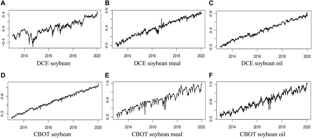
FIGURE 5. The comprehensive investor sentiment index. All comprehensive investor sentiment indexes have upward trends from (A–F).

The Ensemble Empirical Mode Decomposition

Ensemble empirical mode decomposition (EEMD) method is developed from the empirical mode decomposition (EMD) method, which can decompose any set of time series into several simple components of different frequencies and amplitudes (called eigenmode functions sequence) and a residual item [36]. The eigenmode functions sequence can be indicated as IMF. For a set of time series data x(t), the steps of EEMD are as follows.

Step 1: A gaussian white noise sequence ε_l(t) $\left(1\le l\le L\right)$ is added into x(t). The new sequence $x_l\left(t\right)$ can be written as expression (32).

$x_l\left(t\right)=x\left(t\right)+{\epsilon }_l\left(t\right)(32)$

Step 2: According to the principle of EMD, $x_l\left(t\right)$ is decomposed into K IMFs $\left(1\le k\le K\right)$ and a remaining term $r_l\left(t\right)$, seen from expression (33).

$X\left(t\right)={\displaystyle \sum _{k=1}^K{C}_{\left(l, k\right)}}\left(t\right)+r_l\left(t\right)(33)$

Step 3: As the mean value of Gaussian white noise is zero, the influence of adding Gaussian white noise on the IMF can be eliminated. The kth IMF and the remaining term after EEMD decomposition can be shown as expressions (34) and (35).

$c_k\left(t\right)=\frac{1}{L}{\displaystyle \sum _{l=1}^L{C}_{\left(l, k\right)}}\left(t\right)(34)$

$r\left(t\right)=\frac{1}{L}{\displaystyle \sum _{l=1}^L{r}_1}\left(t\right)(35)$

Finally, x(t) can be represented as the sum of K IMFs and a remaining term, seen from expression (36).

$x\left(t\right)={\displaystyle \sum _{k=1}^K{C}_k}\left(t\right)+r\left(t\right)(36)$

To remove the upward trend of ISI sequences in Figure 5, the EEMD model analyzes ISI sequences. According to the signal decomposition results, the eigenmode function sequence and residual sequence are obtained from the six investor sentiment indexes, as shown in Figure 6.

FIGURE 6

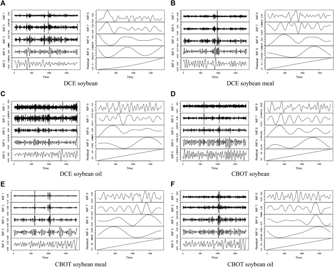
FIGURE 6. The ensemble empirical mode decomposition. Each panel includes nine IMFs and one residual sequence (a trend item). Because all residual sequences have an upward trend, they will be removed to eliminate the influence of trend terms. (A–C) show the results of the ensemble empirical mode decomposition in DCE, and (D–F) show the results of the ensemble empirical mode decomposition in CBOT.

Each ISI is decomposed into a high-frequency sequence, a low-frequency sequence, and a trend item. First, the high-frequency sequence includes IMF1, IMF2, IMF3, IMF4, and IMF5. Second, the low-frequency sequence has IMF6, IMF7, IMF8, and IMF9. Third, the trend item is the residual sequence.

The high-frequency and low-frequency components of comprehensive investor sentiment, written as HIS and LIS, are shown in Figure 7.

FIGURE 7

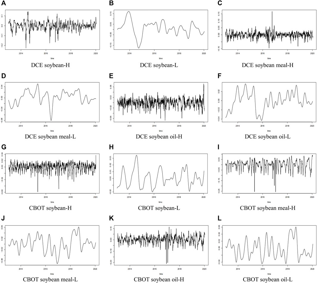
FIGURE 7. The high-frequency and low-frequency components of comprehensive investor sentiment. The letters H and L distinguish the high-frequency and low-frequency components in all panels, respectively. (A–F) show the different components of comprehensive investor sentiment in DCE, and (G–L) show the different components of comprehensive investor sentiment in CBOT.

The Dynamic Correlation of Bean Futures Price Index and Comprehensive Investor Sentiment

The ADF and Granger causality tests are conducted for DCC, HIS, and LIS. The results of the ADF test show that all series are stable, and the p-value of each series is less than 0.05. In Table 13, the dynamic correlation of the bean futures price index is the Granger cause for the low-frequency component of the investor sentiment index in DCE and CBOT.

TABLE 13

TABLE 13. The F-value of Granger causality test.

In order to determine the lag order of the VAR model, the best lag order of the VAR model is tested according to the AIC criterion. The results are shown in Table 14.

TABLE 14

TABLE 14. The lag order of the AIC standard test.

Then sequence auto-correlation tests and stability tests are performed, based on the obtained VAR models. The auto-correlation test results can be seen in Table 15. It is noticed that all p-value are greater than 0.05 in the sequence auto-correlation test (LM test).

TABLE 15

TABLE 15. The results of auto-correlation test.

In order to study the dynamic impacts between the change in investor sentiment and the correlation of the China-US bean futures price index, the impulse response analysis is shown in Figure 8.

FIGURE 8

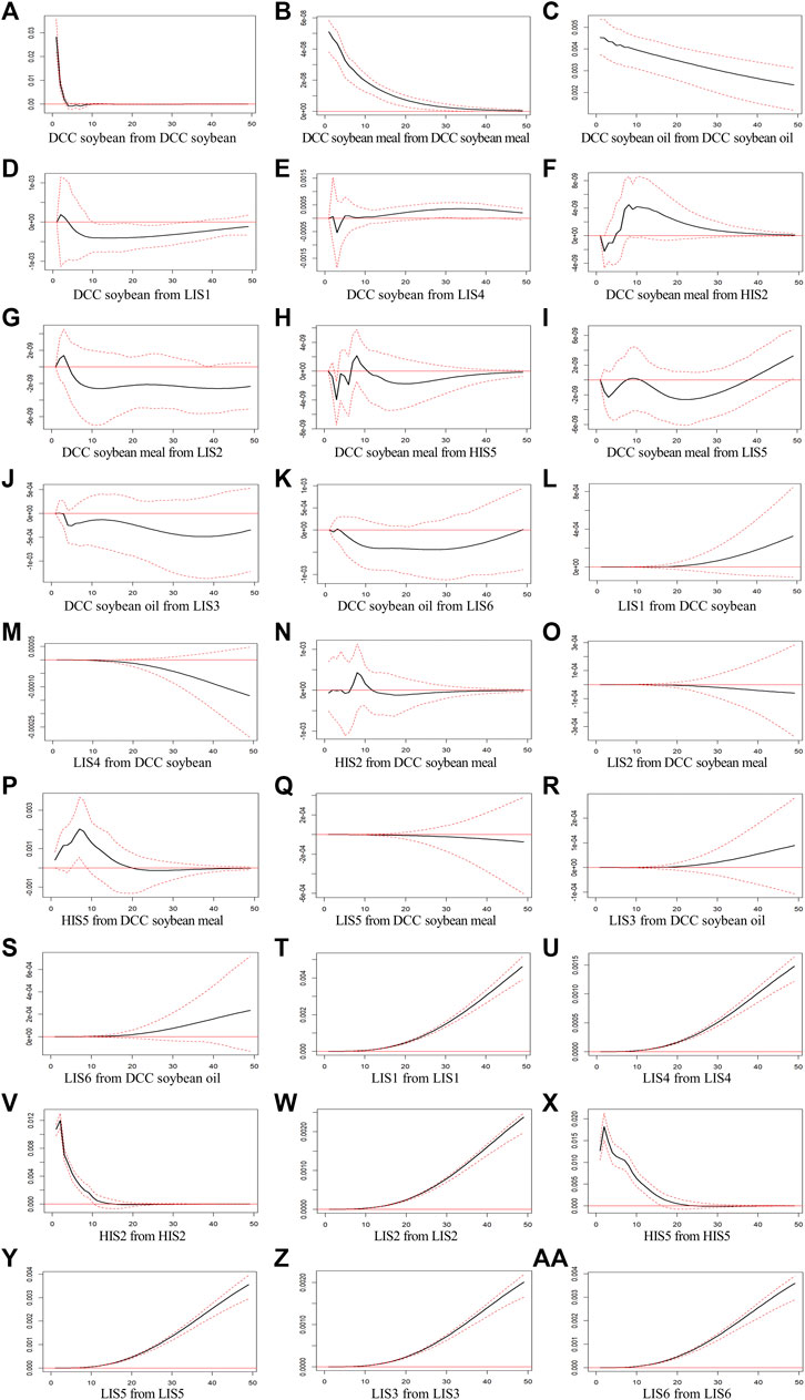
FIGURE 8. The impulse response analysis shows the dynamic impacts between the change in investor sentiment and the dynamic correlation coefficient of the China-US bean futures price index. (A–C) show the response of the dynamic correlation coefficient of the bean futures price index to its shock. (D–K) show the response of the dynamic correlation coefficient of the bean futures price index to the shock of the component of the comprehensive investor sentiment index. (L–S) show the response of the component of the comprehensive investor sentiment index to the shock of the dynamic correlation coefficient of the bean futures price index. (T-AA) show the response of the comprehensive investor sentiment component to its shocks. IS1, IS2 and IS3, respectively, represent the investor sentiment index in Chinese soybean, soybean meal and soybean oil futures markets. Besides, IS4, IS5 and IS6 indicate the investor sentiment index in the US soybean, soybean meal and soybean oil futures markets.

The first step is to study the response of the dynamic correlation coefficient of the bean futures price index to its shock. The dynamic correlation coefficient fluctuates at 2.82% in the first period for soybean futures, then gradually approaches zero in the third period. And the dynamic correlation coefficient produces positive volatility close to zero in the first period for soybean meal futures and gradually becomes zero in the third period. For soybean oil futures, the dynamic correlation coefficient makes a fluctuation of 0.45% in the first period, and then gradually decreases to a very small value close to zero.

The second step is to study the response of the dynamic correlation coefficient of the bean futures price index to the shock of the component of the comprehensive investor sentiment index. For soybean futures markets, the dynamic correlation coefficient produces a fluctuation of 0.02% in the second period, and gradually becomes a negative response in a way approaching zero, after the shock of the low-frequency component in DCE. In CBOT, a fluctuation of 0.0067% occurs in the second period and produces a negative response in the third and fourth periods, a positive response in the fifth period. After reaching the maximum in the thirty-third period, it gradually decreases to a small value approaching zero. The dynamic correlation coefficient fluctuates around zero for soybean meal futures markets with a small amplitude after the shock of the low-frequency and high-frequency components in DCE and CBOT. For soybean oil futures markets, after being impacted by a standard deviation of the low-frequency component in DCE, the dynamic correlation coefficient produces a fluctuation of 0.0008% in the second period and a negative response of 0.0010% in the third period. In CBOT, it has negative volatility of 0.0042% in the second period, a positive response in the third period, a negative response in the fourth period, and then gradually decreases a small value approaching zero in the fiftieth period.

The third step is to study the response of the component of the comprehensive investor sentiment index to the shock of the dynamic correlation coefficient of the bean futures price index. The low-frequency component in DCE and CBOT respectively produces a positive response and a negative response for soybean futures markets. With the response time passing, the comprehensive investor sentiment index has greater changes in these two markets. For soybean meal futures markets, the low-frequency component in DCE and CBOT responds with an increasing trend. In addition, the high-frequency component in DCE produces a negative response of 0.0067% in the first period, and then fluctuates around zero. The high-frequency component in CBOT has a response of 0.041% in the first period and reaches a maximum of 0.2% in the seventh period. Finally, for soybean oil futures markets in DCE and CBOT, the low-frequency component produces a positive response with an increasing trend.

The fourth step is to study the response of the comprehensive investor sentiment component to its shocks. Except for the high-frequency component in soybean meal futures markets, other low-frequency components in other markets can produce a positive response with an increasing trend. For soybean meal markets, the high-frequency component in DCE is affected by a standard deviation of itself, and it produces volatility of 1.08% in the first period, volatility of 1.2% in the second period, and then gradually approaches zero. And the high-frequency component in CBOT, after being impacted by a standard deviation of itself, produces volatility of 1.27% in the first period, a maximum of 1.82% in the second period, and then gradually becomes zero.

Conclusion

With the continuous expansion of China’s agricultural openness, the linkage between the China-US bean futures markets is gradually strengthened. Under the influence of investor sentiment in financial markets, the spillover effect and dynamic correlation of the China-US bean futures markets show some new characteristics. In this paper, we use the BEKK-GARCH model to analyze the spillover effect of the China-US bean futures markets, and choose the DCC-GARCH model to discuss the dynamic correlation coefficients of the China-US bean futures markets. After constructing the high-frequency and low-frequency components of comprehensive investor sentiment, we further study the dynamic impacts between the change in investor sentiment and the correlation of the China-US bean futures price index. Finally, this paper finds that different spillover effects and dynamic correlation coefficients exist between the China-US bean futures markets. Especially, a certain degree of interaction exists between the high-frequency and low-frequency components of the comprehensive investor sentiment index and the dynamic correlation of bean futures price indexes.

Although this paper studies the spillover effect and dynamic correlation based on investor sentiment, the dynamic changes in bean futures markets are incredibly complex. In the future work, we will focus on the influence of information shock on spillover effects between the China-US bean futures markets from a micro point of view, and the dynamic correlation under the China-US financial regulatory policies from a macro point of view. Additionally, we should also pay attention to the influence of the changes in the exchange rate on the spillover effect and dynamic correlation between the China-US bean futures markets.

Data Availability Statement

Publicly available datasets were analyzed in this study. This data can be found here: https://www.wind.com.cn/.

Author Contributions

Conceptualization, TW; methodology, TW; formal analysis, BW; investigation, TW; data curation, TW; writing—original draft preparation, BW and TW; writing—review and editing, BW; supervision, BW; project administration, BW; funding acquisition, BW.

Funding

This research is supported by the National Social Science Fund of China (Grant No. 21XJY014).

Conflict of Interest

The authors declare that the research was conducted in the absence of any commercial or financial relationships that could be construed as a potential conflict of interest.

Publisher’s Note

All claims expressed in this article are solely those of the authors and do not necessarily represent those of their affiliated organizations, or those of the publisher, the editors and the reviewers. Any product that may be evaluated in this article, or claim that may be made by its manufacturer, is not guaranteed or endorsed by the publisher.

References

1. Beckmann J, Czudaj R. Volatility Transmission in Agricultural Futures Markets. Econ Model (2014) 36:541–6. doi:10.1016/j.econmod.2013.09.036

CrossRef Full Text | Google Scholar

2. Jia R-L, Wang D-H, Tu J-Q, Li S-P. Correlation between Agricultural Markets in Dynamic Perspective-Evidence from China and the US Futures Markets. Physica A: Stat Mech its Appl (2016) 464:83–92. doi:10.1016/j.physa.2016.07.048

CrossRef Full Text | Google Scholar

3. Guo ZY. How Information Is Transmitted across the Nations? an Empirical Investigation of the US and Chinese Commodity Markets. Glob J. Manag. Bus. Res. (2017) 17:1–11.

Google Scholar

4. Ruan Q, Cui H, Fan L. China's Soybean Crush Spread: Nonlinear Analysis Based on MF-DCCA. Physica A: Stat Mech its Appl (2020) 554:123899. doi:10.1016/j.physa.2019.123899

CrossRef Full Text | Google Scholar

5. He R, Zhu D, Chen X, Cao Y, Chen Y, Wang X. How the Trade Barrier Changes Environmental Costs of Agricultural Production: An Implication Derived from China's Demand for Soybean Caused by the US-China Trade War. J Clean Prod (2019) 227:578–88. doi:10.1016/j.jclepro.2019.04.192

CrossRef Full Text | Google Scholar

6. Chen Z, Yan B. The Impact of Trade Policy on Soybean Futures in China. Manage Decis Econ (2021), 1–12. doi:10.1002/mde.3446

CrossRef Full Text | Google Scholar

7. Mahadi MI, Mahmood WMW, Ismail F. Dynamic Cross-Market Linkages of Commodity Futures Markets: Evidence from FCPO and DCE. J Appl Environ Biol Sci (2014) 4:41–6.

Google Scholar

8. Mukherjee I, Goswami B. The Volatility of Returns from Commodity Futures: Evidence from India. Financ Innov (2017) 3:1–23. doi:10.1186/s40854-017-0066-9

CrossRef Full Text | Google Scholar

9. Thiyagarajan S, Mahalakshmi S, Kirithiga S, Naresh G. Price Dissemination of International and Domestic Commodity Markets. Ijbd (2021) 4:179–95. doi:10.1504/IJBD.2021.116959

CrossRef Full Text | Google Scholar

10. Margarido MA, Turolla FA, Bueno CRF. The World Market for Soybeans: price Transmission into Brazil and Effects from the Timing of Crop and Trade. Nova Econ (2007) 17:1–19. doi:10.1590/s0103-63512007000200002

CrossRef Full Text | Google Scholar

11. Liu Q, An Y. Information Transmission in Informationally Linked Markets: Evidence from US and Chinese Commodity Futures Markets. J Int Money Finance (2011) 30:778–95. doi:10.1016/j.jimonfin.2011.05.006

CrossRef Full Text | Google Scholar

12. Ji Q, Zhang X, Zhu Y. Multifractal Analysis of the Impact of US-China Trade Friction on US and China Soy Futures Markets. Physica A: Stat Mech its Appl (2020) 542:123222. doi:10.1016/j.physa.2019.123222

CrossRef Full Text | Google Scholar

13. Ajoy Kumar M, Shollapur MR. Price Discovery and Spillover in the Agricultural Commodity Futures Market in India. IUP J Ppl Financ (2015) 21:54–70.

Google Scholar

14. Etienne XL, Trujillo-Barrera A, Hoffman LA. Volatility Spillover and Time-Varying Conditional Correlation between DDGS, Corn, and Soybean Meal Markets. Agric Resour Econom Rev (2017) 46:529–54. doi:10.1017/age.2016.44

CrossRef Full Text | Google Scholar

15. Dahl RE, Oglend A, Yahya M. Dynamics of Volatility Spillover in Commodity Markets: Linking Crude Oil to Agriculture. J Commodity Markets (2020) 20:100111. doi:10.1016/j.jcomm.2019.100111

CrossRef Full Text | Google Scholar

16. Li J. The Effect of Oil price on China's Grain Prices: a VAR Model. Adv Manag Appl Econ (2021) 11:91–100. doi:10.47260/amae/1115

CrossRef Full Text | Google Scholar

17. Liu X-d., Pan F, Yuan L, Chen Y-w.. The Dependence Structure between Crude Oil Futures Prices and Chinese Agricultural Commodity Futures Prices: Measurement Based on Markov-Switching GRG Copula. Energy (2019) 182:999–1012. doi:10.1016/j.energy.2019.06.071

CrossRef Full Text | Google Scholar

18. Yu THE, Bessler DA, Fuller SW. Cointegration and Causality Analysis of World Vegetable Oil and Crude Oil Prices. In: 2006 Annual meeting; July 23-26; Long Beach, CA 21439. American Agricultural Economics Association (2006). doi:10.22004/ag.econ.21439

CrossRef Full Text | Google Scholar

19. Zhang Z, Lohr L, Escalante C, Wetzstein M. Ethanol, Corn, and Soybean price Relations in a Volatile Vehicle-Fuels Market. Energies (2009) 2:320–39. doi:10.3390/en20200320

CrossRef Full Text | Google Scholar

20. Han L, Jin J, Wu L, Zeng H. The Volatility Linkage between Energy and Agricultural Futures Markets with External Shocks. Int Rev Financial Anal (2020) 68:101317. doi:10.1016/j.irfa.2019.01.011

CrossRef Full Text | Google Scholar

21. Jiang J, Fortenbery TR. El Niño and La Niña Induced Volatility Spillover Effects in the U.S. Soybean and Water Equity Markets. Appl Econ (2019) 51:1133–50. doi:10.1080/00036846.2018.1524980

CrossRef Full Text | Google Scholar

22. Fernandes LHS, Araújo FHA. Taxonomy of Commodities Assets via Complexity-Entropy Causality Plane. Chaos, Solitons & Fractals (2020) 137:109909. doi:10.1016/j.chaos.2020.109909

CrossRef Full Text | Google Scholar

23. Araujo FHA, Fernandes LHS. Lighting the Populational Impact of COVID-19 Vaccines in Brazil. Fractals (2022), 15. Accepted Paper. doi:10.1142/S0218348X22500669

CrossRef Full Text | Google Scholar

24. Xu Q, Wang L, Jiang C, Zhang X. A Novel UMIDAS-SVQR Model with Mixed Frequency Investor Sentiment for Predicting Stock Market Volatility. Expert Syst Appl (2019) 132:12–27. doi:10.1016/j.eswa.2019.04.066

CrossRef Full Text | Google Scholar

25. Wu B, Cai Y, Zhang M. Investor Sentiment and Stock price Crash Risk in the Chinese Stock Market. J Maths (2021) 2021:1–10. doi:10.1155/2021/6806304

CrossRef Full Text | Google Scholar

26. Zaremba A, Szczygielski JJ. Limits to Arbitrage, Investor Sentiment, and Factor Returns in International Government Bond Markets. Econ Research-Ekonomska Istraživanja (2019) 32:1727–43. doi:10.1080/1331677X.2019.1638286

CrossRef Full Text | Google Scholar

27. Engle RF, Kroner KF. Multivariate Simultaneous Generalized ARCH. Econom Theor (1995) 11:122–50. doi:10.1017/S0266466600009063

CrossRef Full Text | Google Scholar

28. Alkan B, Çiçek S. Spillover Effect in Financial Markets in Turkey. Cent Bank Rev (2020) 20:53–64. doi:10.1016/j.cbrev.2020.02.003

CrossRef Full Text | Google Scholar

29. Huang Y, Su W, Li X. Comparison of BEKK GARCH and DCC GARCH Models: An Empirical Study. In: Proceedings of International Conference on Advanced Data Mining and Applications; 2010 November 19-21; Chongqing, China. Berlin, Heidelberg: Springer (2010). p. 99–110. doi:10.1007/978-3-642-17313-4_10

CrossRef Full Text | Google Scholar

30. Pedersen RS, Rahbek A. Multivariate Variance Targeting in the BEKK-GARCH Model. Econom J (2014) 17:24–55. doi:10.1111/ectj.12019

CrossRef Full Text | Google Scholar

31. Zhipeng Y, Shenghong L. Hedge Ratio on Markov Regime-Switching diagonal Bekk-Garch Model. Finance Res Lett (2018) 24:49–55. doi:10.1016/j.frl.2017.06.015

CrossRef Full Text | Google Scholar

32. Wu D, Hu Z-h.. Structural Changes and Volatility Correlation in Nonferrous Metal Market. Trans Nonferrous Met Soc China (2016) 26:2784–92. doi:10.1016/S1003-6326(16)64395-9

CrossRef Full Text | Google Scholar

33. Celık S. The More Contagion Effect on Emerging Markets: The Evidence of DCC-GARCH Model. Econ Model (2012) 29:1946–59. doi:10.1016/j.econmod.2012.06.011

CrossRef Full Text | Google Scholar

34. Jones PM, Olson E. The Time-Varying Correlation between Uncertainty, Output, and Inflation: Evidence from a DCC-GARCH Model. Econ Lett (2013) 118:33–7. doi:10.1016/j.econlet.2012.09.012

CrossRef Full Text | Google Scholar

35. Stošić D, Stošić D, Stošić T, Eugene Stanley H. Multifractal Properties of price Change and Volume Change of Stock Market Indices. Physica A: Stat Mech its Appl (2015) 428:46–51. doi:10.1016/j.physa.2015.02.046

CrossRef Full Text | Google Scholar

36. Wu Z, Huang NE. Ensemble Empirical Mode Decomposition: A Noise-Assisted Data Analysis Method. Adv Adapt Data Anal (2009) 01:1–41. doi:10.1142/S1793536909000047

CrossRef Full Text | Google Scholar