Two Novel One-Way Delay Clock Skew Estimators and Their Performances for the Fractional Gaussian Noise/Generalized Fractional Gaussian Noise Environment Applicable for the IEEE 1588v2 (PTP) Case

Papers in the literature dealing with the Ethernet network characterize packet delay variation (PDV) as a long-range dependence (LRD) process. The fractional Gaussian noise (fGn) or the generalized fractional Gaussian noise (gfGn) belong to the LRD process. The IEEE1588v2 is a two-way delay (TWD) protocol that uses the messages from the Forward (Master to Slave) and the Reverse (Slave to Master) paths. Suppose we have a significant difference between the PDV variances of the Forward and the Reverse paths. Thus, if we can use only the path with the lowest PDV variance (namely, only the one-way delay (OWD) technique), we might get a better clock skew performance from the mean square error (MSE) point of view compared with the traditional TWD method. This paper proposes two OWD clock skew estimators, one for the Forward path and one for the Reverse path applicable for the white-Gaussian, fGn and gfGn environment. Those OWD estimators do not depend on the unknown asymmetry between the fixed delays in the Forward and Reverse paths and nor on the clock offset between the Master and Slave. We also supply two closed-form approximated expressions for the MSE related to our new proposed OWD clock skew estimators. In addition, we supply some conditions, summarized in a table, guiding us whether we should use the OWD clock skew estimator for the Forward path or for the Reverse path, or just use the TWD algorithm. Simulation results confirm that our new proposed OWD clock skew estimators achieve better clock skew performances from the MSE point of view, compared with the TWD clock skew estimator recently proposed by the same authors and compared with two literature known OWD methods (the maximum likelihood and Kalman clock skew estimators).

1 Introduction

The Precision Time Protocol (PTP), named also as the IEEE 1588v2 standard [1] is a TWD exchange scheme where the Slave exchanges a series of synchronization packets with its Master so the packet timestamps can be employed to estimate the clock skew relative to the Master. In other words, the PTP as a TWD algorithm uses messages received from the Forward (Master to Slave) and from the Reverse (Slave to Master) paths in order to estimate the clock skew relative to the Master. The synchronization packets can encounter several intermediate switches and routers along the network path between the Master and the Slave [2]. Networks often suffer large unpredictable queuing delays at switches and routers (thus having heavy PDV in the network) due to the presence of background traffic [3]. This background traffic may be a real traffic or one caused by a cyber attack [2] where a malicious intermediate node deliberately delays the transmission of synchronization messages. A heavy PDV can be seen in the Forward path, in the Reverse path or in both paths. Usually, the PDV in the Forward path is different from the PDV in the Reverse path. The problem is that the PDV of the Forward and Reverse paths can significantly hamper the accuracy of the clock skew estimation [3]. A lower PDV will lead to a more accurate clock skew estimation compared to a higher PDV. Thus, if the difference in the PDVs encountered in Forward and Reverse paths is high, the clock skew estimation accuracy obtained with the TWD technique is mainly decreased due to the path with the higher PDV. Thus, if we could use for the clock skew estimation task only the path with the lowest PDV (namely, using the OWD technique), the clock skew performance from the MSE point of view might be improved compared with the case where we have also to consider the path with the higher PDV (the TWD approach). Since the lower PDV path may occur in the Forward path as well as in the Reverse path, two different OWD clock skew estimators are needed (one for the Forward path and the other one associated with the Reverse path). So far we have seen that for the clock skew estimation task, the OWD technique may be more useful compared with the TWD approach in cases where the Forward PDV variance is very different from the Reverse PDV variance. According to [4], PTP (which is a TWD exchange scheme) has more unknown parameters than available equations. Thus, in order to solve the problem, a symmetric path is usually assumed. Namely, the fixed delay in the Forward path is usually assumed to be the same as the fixed delay for the Reverse path. But, in practical scenarios, this is not the case. Thus, for an asymmetrical path, when the symmetric path assumption is applied, a degradation in the clock skew estimation may be obtained when the TWD approach is applied. Now, the OWD technique relies only on one path, on the Reverse path or on the Forward path. Thus, the symmetric assumption is not needed in the OWD technique which can be considered here as an advantage compared with the TWD approach. Suppose for a moment that we have three clock skew estimators applicable for the PTP case. Namely, we have one OWD clock skew estimator for the Forward path, one OWD clock skew estimator for the Reverse path and a TWD clock skew estimator. Next we wish to know which of the three clock skew estimators should be taken for the clock skew estimation task given a network where different PDV variances are seen on both Forward and Reverse paths but the fixed delay of the Forward path is equal to the fixed delay of the Reverse path. It is quite reasonable to think that when the Forward path PDV variance is equal or close to equal to the Reverse path PDV variance, the TWD clock skew estimator is preferable over the OWD clock skew estimator due to the “averaging” effect of the variances in the TWD clock skew estimator. But, when the PDV variances of the Forward and Reverse paths are different and on the same time the difference in the variances is not very high, it is not clear if the OWD clock skew estimator for the Forward path or the OWD clock skew estimator for the Reverse path or maybe the TWD clock skew estimator should be applied for the clock skew estimation task. Thus, some guiding lines (closed-form expressions, conditions) are needed here, telling us which approach should be applied in order to get the best clock skew performance in the MSE point of view. Namely, which clock skew estimator should be taken: the OWD clock skew estimator for the Forward path or the OWD clock skew estimator for the Reverse path or perhaps the TWD clock skew estimation approach. Recently [4], we proposed a new TWD clock skew estimator for the PTP case that has the best clock skew performance in the MSE point of view compared to the relevant literature known estimators [5–7]. This clock skew estimator [4] is suitable for the white-Gaussian and fGn/gfGn cases and does not depend on the asymmetric fixed delay between the Forward and the Reverse paths, nor on the offset between the Master and the Slave clocks. This paper is a direct continuation of our previous work [4]. Thus, please refer to [4] in order to find a detailed overview of the existing TWD and recently proposed OWD approaches for the PTP case. Please note that the two recently proposed OWD clock skew estimators [6,7], are both OWD clock skew estimators associated with the Forward path. Thus, if the Forward path PDV variance is much higher compared with the Reverse path PDV variance, [6,7] may not get better clock skew performance from the MSE point of view compared with the TWD approach and compared with the OWD clock skew estimator associated with the Reverse path. As already was mentioned, this paper is a direct continuation of our previous work [4] where we proposed a novel TWD clock skew estimator applicable for the PTP case. In this paper we propose:

1. A novel OWD clock skew estimator for the Forward path based on [4], applicable for the white-Gaussian and fGn/gfGn environment.

2. A novel OWD clock skew estimator for the Reverse path based on [4], applicable for the white-Gaussian and fGn/gfGn environment.

3. A closed-form-approximated expression for the clock skew performance (MSE) related to our OWD proposed clock skew estimator for the Forward path.

4. A closed-form-approximated expression for the clock skew performance (MSE) related to our OWD proposed clock skew estimator for the Reverse path.

5. Guiding lines (closed-form expressions, conditions), summarized in a table (please refer to Table 1), telling us if we should use the OWD clock skew estimator for the Forward path or the OWD clock skew estimator for the Reverse path or perhaps the TWD clock skew estimator proposed by [4] in order to get the best clock skew performance from the MSE point of view.

TABLE 1

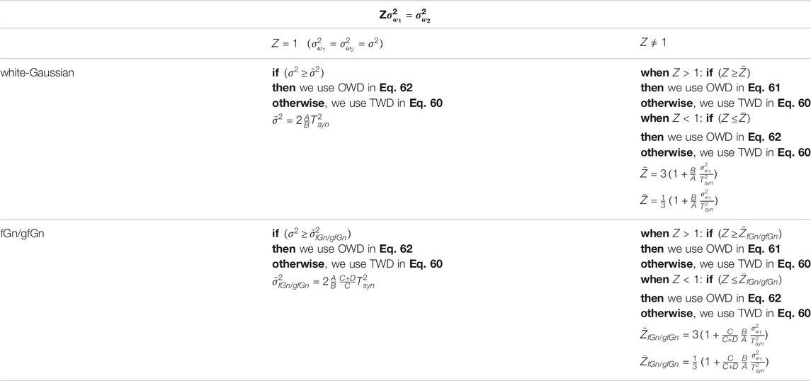
TABLE 1. Summary of the conditions where the suggested estimator have the possible lower MSE.

The clock skew performances (MSE) of our new proposed OWD clock skew estimators were compared via simulation with the clock skew performances (MSE) obtained with two TWD clock skew estimators [4,5] and with the literature known OWD clock skew estimators [6,7]. Simulation results will show the advantage in performance (MSE) of our new proposed OWD clock skew estimators compared to [4–7]. Simulation results will also show the effectiveness of our closed-form-approximated expressions for the clock skew performance (MSE) associated to the Forward and Reverse paths as well as the effectiveness of our proposed guiding lines, leading us to the right choice of the clock skew estimator from the MSE point of view.

The paper is organized as follows. Section 2 briefly introduces the system under consideration and the assumptions we applied for our algorithm. Section 3 proposes the OWD clock skew estimators for the Forward and Reverse paths. Section 4 suggests the closed-form approximated expressions for the MSE related to our new proposed OWD clock skew estimators where the PDV is a white-Gaussian process. Section 5 suggests the closed-form approximated expressions for the MSE related to our new proposed OWD clock skew estimators where the PDV is an fGn/gfGn process. In Section 6, we derive some guiding lines (conditions), summarized in Table 1, telling us under what condition should we prefer the OWD for the Forward path over the OWD for the Reverse path or should just prefer the TWD clock skew estimator obtained in [4]. Section 7 presents simulation results, and in Section 8, a conclusion is given.

2 System Description

As already was mentioned earlier, this paper is a direct continuation of our previous work [4]. Thus, the system description is the same as in [4]. Please refer to [4], for having a detailed description of the message exchange flow between the Master and the Slave. Let us recall Figure 1 from [4] where based on [8–10] we may write:

$t_1\left[j\right]+d_{ms}+{\omega }_1\left[j\right]=t_2\left[j\right]\left(1+\alpha \right)+Q(1)$

$t_4\left[j\right]-d_{sm}-{\omega }_2\left[j\right]=t_3\left[j\right]\left(1+\alpha \right)+Q(2)$

where Q is the time difference between the Master and the Slave clocks (offset) and α is the clock skew. The Forward and the Reverse fixed delays are denoted as d_ms, d_sm respectively. The Forward PDV is denoted as ω₁[j] and the Reverse PDV is denoted as ω₂[j]. The total number of the Sync messages periods is denoted as J, where j = 1, 2, 3, … , J. At timestamp t₁, the Master sends a Sync message to the Slave. The Slave receives this Sync message at timestamp t₂ and sends back to the Master a Delay Req message at timestamp t₃. The Master receives this Delay Req message at timestamp t₄. Please note that t₁[j], t₂[j], t₃[j], t₄[j] are the timestamps of t₁, t₂, t₃ and t₄ respectively at the jth Sync message period.

FIGURE 1

FIGURE 1. PTP messaging timing diagram.

We consider two different models for the PDV, as was done in [4]:

1. The PDV is modeled as a white-Gaussian noise with zero mean and the variance $E\left[{\omega }_n[j],{\omega }_n[m]\right]$ is ${\sigma }_{{\omega }_n}^2$ when j = m and zero when j ≠ m

where E [.] denotes the expectation operator on (.) and n = 1, 2.

2. The PDV is modeled as an fGn/gfGn process with zero mean. Based on [11–13] we have:

a. When j = m: $E\left[{\omega }_n[j],{\omega }_n[m]\right]={\sigma }_{{\omega }_n}^2$.

b. When j ≠ m: $E\left[{\omega }_n[j],{\omega }_n[m]\right]=\frac{{\sigma }_{{\omega }_n}^2}{2}\left[{\left.‖{(j-m)}^a|-1\right|}^{2H}-2{(|{(j-m)}^a|)}^{2H}+{(|{(j-m)}^a|+1)}^{2H}\right]$.

where a = 1 is the fGn case.

In addition, we use also the same assumptions as were made in [4]:

1. The Forward and the Reverse PDVs are independent. Thus, we have: $E\left[{\omega }_1[j],{\omega }_2[m]\right]=0\forall j,m$.

2. In the Slave clock the time between t₂ [j] to t₃ [j] is constant and is denoted as X. Thus, we have: t₃ [j] − t₂ [j] = X.

In this paper we propose two novel OWD clock skew estimators, one for the Forward path and one for the Reverse path. Both OWD clock skew estimators are based on our previously TWD clock skew estimator [4] given by:

$\widehat{\alpha }=\frac{1}{J\left(J-1\right)}\sum _{i=1}^{J-1}\sum _{j=1}^{J-i}\left(\frac{T_{1,j}\left(i\right)}{T_{2,j}\left(i\right)}+\frac{T_{4,j}\left(i\right)}{T_{2,j}\left(i\right)}\right)-1(3)$

where

$\begin{array}{cc}\hfill & T_{1,j}\left(i\right)=t_1\left[j+i\right]-t_1\left[j\right],T_{2,j}\left(i\right)=t_2\left[j+i\right]-t_2\left[j\right],\hfill \\ \hfill & T_{4,j}\left(i\right)=t_4\left[j+i\right]-t_4\left[j\right]\hfill \end{array}(4)$

3 The OWD Clock Skew Estimators

In the following, we present in Theorem 1 our new proposed OWD clock skew estimator for the Forward path and in Theorem 2 our new proposed OWD clock skew estimator for the Reverse path.

3.1 Theorem 1

The clock skew estimator for the OWD in the Forward path (Master to Slave) can be written as:

${\widehat{\alpha }}^F=\frac{2}{J\left(J-1\right)}\sum _{i=1}^{J-1}\sum _{j=1}^{J-i}\left(\frac{T_{1,j}\left(i\right)}{T_{2,j}\left(i\right)}\right)-1(5)$

where ${\widehat{\alpha }}^F$ is the is the clock skew estimator that based only on timestamps from the Forward path.

Proof of Theorem 1

In order to avoid the fixed delay, we can subtract between two timestamps from different Sync periods. Therefore, based on Eq. 1 we have:

$T_{1,j}\left(i\right)+{\mathrm{\Omega }}_{1,j}\left(i\right)=T_{2,j}\left(i\right)\left(1+{\alpha }_{j,i}^F\right)(6)$

where ${\alpha }_{j,i}^F$ is the clock skew between the (j + i)-th and ith Sync period, and Ω_1,j(i) is:

${\mathrm{\Omega }}_{1,j}\left(i\right)={\omega }_1\left[j+i\right]-{\omega }_1\left[j\right](7)$

Based on Eq. 6 the clock skew can be written as:

${\alpha }_{j,i}^F=\frac{T_{1,j}\left(i\right)}{T_{2,j}\left(i\right)}+\frac{{\mathrm{\Omega }}_{1,j}\left(i\right)}{T_{2,j}\left(i\right)}-1(8)$

The OWD clock skew in the Forward path can be defined as:

${\alpha }^F=\frac{2}{J\left(J-1\right)}\sum _{i=1}^{J-1}\sum _{j=1}^{J-i}{\alpha }_{j,i}^F(9)$

By putting Eq. 8 into Eq. 9 we define the clock skew in the Forward path as:

$\begin{array}{cc}\hfill {\alpha }^F& =\frac{2}{J\left(J-1\right)}\sum _{i=1}^{J-1}\sum _{j=1}^{J-i}\left(\left(\frac{T_{1,j}\left(i\right)}{T_{2,j}\left(i\right)}\right)+\left(\frac{{\mathrm{\Omega }}_{1,j}\left(i\right)}{T_{2,j}\left(i\right)}\right)\right)-1\hfill \\ \hfill & ={\widehat{\alpha }}^F+\frac{2}{J\left(J-1\right)}\sum _{i=1}^{J-1}\sum _{j=1}^{J-i}\left(\frac{{\mathrm{\Omega }}_{1,j}\left(i\right)}{T_{2,j}\left(i\right)}\right)\hfill \end{array}(10)$

This completes our proof.

3.2 Theorem 2

The skew clock estimator for the OWD in the Reverse path (Slave to Master) can be written as:

${\widehat{\alpha }}^R=\frac{2}{J\left(J-1\right)}\sum _{i=1}^{J-1}\sum _{j=1}^{J-i}\left(\frac{T_{4,j}\left(i\right)}{T_{2,j}\left(i\right)}\right)-1(11)$

where ${\widehat{\alpha }}^R$ is the is the clock skew estimator that based only on timestamps from the Reverse path.

Proof of Theorem 2

In order to avoid the fixed delay, we can subtract between two timestamps from different Sync periods. Therefore, based on Eq. 2 we have:

$T_{4,j}\left(i\right)-{\mathrm{\Omega }}_{2,j}\left(i\right)=T_{3,j}\left(i\right)\left(1+{\alpha }_{j,i}^R\right)(12)$

where ${\alpha }_{j,i}^R$ is the clock skew between the (j + i)-th and ith Sync period, and

$T_{3,j}\left(i\right)=t_3\left[j+i\right]-t_3\left[j\right];{\mathrm{\Omega }}_{2,j}\left(i\right)={\omega }_2\left[j+i\right]-{\omega }_2\left[j\right](13)$

Based on the definition that t₃ [j] − t₂ [j] = X, as mentioned in the section of System Description (assumption 2), we can write:

$T_{3,j}\left(i\right)=t_3\left[j+i\right]-t_3\left[j\right]=t_2\left[j+i\right]+X-\left(t_2\left[j\right]+X\right)=T_{2,j}\left(i\right)(14)$

By using Eq. 14, we can write Eq. 12 as:

$T_{4,j}\left(i\right)-{\mathrm{\Omega }}_{2,j}\left(i\right)=T_{2,j}\left(i\right)\left(1+{\alpha }_{j,i}^R\right)(15)$

Therefore, based on Eq. 15 the clock skew can be written as:

${\alpha }_{j,i}^R=\frac{T_{4,j}\left(i\right)}{T_{2,j}\left(i\right)}-\frac{{\mathrm{\Omega }}_{2,j}\left(i\right)}{T_{2,j}\left(i\right)}-1(16)$

The OWD clock skew in the Reverse path can be defined as:

${\alpha }^R=\frac{2}{J\left(J-1\right)}\sum _{i=1}^{J-1}\sum _{j=1}^{J-i}{\alpha }_{j,i}^R(17)$

By putting Eq. 16 into Eq. 17 we define the clock skew in the Reverse path as:

$\begin{array}{cc}\hfill {\alpha }^R& =\frac{2}{J\left(J-1\right)}\sum _{i=1}^{J-1}\sum _{j=1}^{J-i}\left(\left(\frac{T_{4,j}\left(i\right)}{T_{2,j}\left(i\right)}\right)-\left(\frac{{\mathrm{\Omega }}_{2,j}\left(i\right)}{T_{2,j}\left(i\right)}\right)\right)-1\hfill \\ \hfill & ={\widehat{\alpha }}^R-\frac{2}{J\left(J-1\right)}\sum _{i=1}^{J-1}\sum _{j=1}^{J-i}\left(\frac{{\mathrm{\Omega }}_{2,j}\left(i\right)}{T_{2,j}\left(i\right)}\right)\hfill \end{array}(18)$

This completes our proof.

4 The Clock Skew Performance for the White-Gaussian Case

In the following, Theorems 3 and 4 present the closed-form approximated expressions for the MSE related to our new proposed OWD clock skew estimator for the Forward path and Reverse path, respectively. According to [4], the MSE for the TWD clock skew estimator for the Gaussian case is given by:

$E\left[e^2\right]\approx {\left(\frac{1}{J\left(J-1\right)}\right)}^2\left[\frac{\left({\sigma }_{{\omega }_1}^2+{\sigma }_{{\omega }_2}^2\right)}{T_{syn}^2}A\left(1+\frac{1}{P}\right)\right](19)$

where P is:

$P=\frac{A}{B}\left(\frac{{\sigma }_{{\omega }_1}^2+{\sigma }_{{\omega }_2}^2}{{\sigma }_{{\omega }_1}^4}\right)T_{syn}^2(20)$

and A, B are given by:

$A=\left(2\sum _{i=1}^{J-1}\frac{J-i}{i^2}+\sum _{i=1}^{J-1}\sum _{j=1}^{J-i}\sum _{\begin{array}{c}k=1\\ k\ne i\end{array}}^{J-1}\sum _{\begin{array}{c}m=1\\ m=j\\ m=j+i-k\end{array}}^{J-k}\frac{1}{ik}-\sum _{i=1}^{J-1}\sum _{j=1}^{J-i}\sum _{\begin{array}{c}k=1\end{array}}^{J-1}\sum _{\begin{array}{c}m=1\\ m=j+i\\ m=j-k\end{array}}^{J-k}\frac{1}{ik}\right)(21)$

$B=\left(12\sum _{i=1}^{J-1}\frac{J-i}{i^4}+6\sum _{i=1}^{J-1}\sum _{j=1}^{J-i}\sum _{\begin{array}{c}k=1\\ k\ne i\end{array}}^{J-1}\sum _{\begin{array}{c}m=1\\ m=j\\ m=j+i-k\\ m=j+i\\ m=j-k\end{array}}^{J-k}\frac{1}{{\left(ik\right)}^2}+4\sum _{i=1}^{J-1}\sum _{j=1}^{J-i}\sum _{\begin{array}{c}k=1\end{array}}^{J-1}\sum _{\begin{array}{c}m=1\\ m\ne j\\ m\ne j+i-k\\ m\ne j+i\\ m\ne j-k\end{array}}^{J-k}\frac{1}{{\left(ik\right)}^2}\right)(22)$

4.1 Theorem 3

For $\left|\frac{{\mathrm{\Omega }}_{1,j}(i)}{T_{1,j}(i)}\right|\ll 1$, the closed-form-approximated expression for the MSE related to the OWD clock skew estimator (for the Forward path), can be defined as:

$E\left[e_F^2\right]\approx {\left(\frac{2}{\left(J\left(J-1\right)\right)}\right)}^2\left[\frac{{\sigma }_{{\omega }_1}^2}{T_{syn}^2}A\left(1+\frac{1}{P_F}\right)\right](23)$

where P_F is:

$P_F=\frac{A}{B}\left(\frac{T_{syn}^2}{{\sigma }_{{\omega }_1}^2}\right)(24)$

where A and B are defined in Eq. 21, 22 respectively.

Proof of Theorem 3

Based on Eq. 10 the error of the OWD clock skew estimator (for the Forward path) is:

$e_F={\alpha }_F-{\widehat{\alpha }}_F=\frac{2}{J\left(J-1\right)}\sum _{i=1}^{J-1}\sum _{j=1}^{J-i}\left(\frac{{\mathrm{\Omega }}_{1,j}\left(i\right)}{T_{2,j}\left(i\right)}\right)(25)$

Now, according to Eq. 6 we can write T_2,j(i) as following:

$T_{2,j}\left(i\right)=\frac{T_{1,j}\left(i\right)+{\mathrm{\Omega }}_{1,j}\left(i\right)}{\left(1+{\alpha }_{j,i}^F\right)}(26)$

Based on Eq. 26 we may write the expectation of Eq. 25 as:

$E\left[e_F\right]=\frac{2\left(1+{\alpha }^F\right)}{\left(J\left(J-1\right)\right)}\sum _{i=1}^{J-1}\sum _{j=1}^{J-i}E\left[\frac{a_{j,i}}{\left(1+a_{j,i}\right)}\right](27)$

where

$a_{j,i}=\frac{{\mathrm{\Omega }}_{1,j}\left(i\right)}{T_{1,j}\left(i\right)}(28)$

For $\left|\frac{{\mathrm{\Omega }}_{1,j}(i)}{T_{1,j}(i)}\right|\ll 1$ we can write Eq. 27 as:

$E\left[e_F\right]\approx \frac{2\left(1+{\alpha }^F\right)}{\left(J\left(J-1\right)\right)}\sum _{i=1}^{J-1}\sum _{j=1}^{J-i}\left[E\left[a_{j,i}\left(1-a_{j,i}\right)\right]\right](29)$

Based on Eq. 29 the approximated MSE related to the OWD clock skew estimator (for the Forward path) can be define as:

$\begin{array}{c}\hfill E\left[e_F^2\right]\approx \frac{4{\left(1+{\alpha }^F\right)}^2}{{\left(J\left(J-1\right)\right)}^2}\sum _{i=1}^{J-1}\sum _{j=1}^{J-i}\sum _{k=1}^{J-1}\sum _{j=m}^{J-k}\\ \hfill \left[E\left[a_{j,i}{a}_{m,k}\right]-E\left[a_{j,i}^2{a}_{m,k}\right]-E\left[a_{j,i}{a}_{m,k}^2\right]+E\left[a_{j,i}^2{a}_{m,k}^2\right]\right]\end{array}(30)$

According to [4], we can write T_1,j(i) and T_1,m(k) as:

$\begin{array}{c}\hfill T_{1,j}\left(i\right)=t_1\left[j+i\right]-t_1\left[j\right]=i{T}_{syn}\\ \hfill T_{1,m}\left(k\right)=t_1\left[m+k\right]-t_1\left[m\right]=k{T}_{syn}\end{array}(31)$

where T_syn is the Sync messages period.

Based on Eq. 28 and on Eq. 31 we can simplify the expressions in Eq. 30:

$E\left[a_{j,i}{a}_{m,k}\right]=E\left[\frac{{\mathrm{\Omega }}_{1,j}\left(i\right)}{T_{1,j}\left(i\right)}\frac{{\mathrm{\Omega }}_{1,m}\left(k\right)}{T_{1,m}\left(k\right)}\right]=\frac{E\left[{\mathrm{\Omega }}_{1,j}\left(i\right){\mathrm{\Omega }}_{1,m}\left(k\right)\right]}{ik{T}_{syn}^2}(32)$

$E\left[a_{j,i}^2{a}_{m,k}\right]=E\left[\frac{{\mathrm{\Omega }}_{1,j}^2\left(i\right)}{T_{1,j}^2\left(i\right)}\frac{{\mathrm{\Omega }}_{1,m}\left(k\right)}{T_{1,m}\left(k\right)}\right]=\frac{E\left[{\mathrm{\Omega }}_{1,j}^2\left(i\right){\mathrm{\Omega }}_{1,m}\left(k\right)\right]}{i^{2}k{T}_{syn}^3}(33)$

$E\left[a_{j,i}{a}_{m,k}^2\right]=E\left[\frac{{\mathrm{\Omega }}_{1,j}\left(i\right)}{T_{1,j}\left(i\right)}\frac{{\mathrm{\Omega }}_{1,m}^2\left(k\right)}{T_{1,m}^2\left(k\right)}\right]=\frac{E\left[{\mathrm{\Omega }}_{1,j}\left(i\right){\mathrm{\Omega }}_{1,m}^2\left(k\right)\right]}{i{k}^2{T}_{syn}^3}(34)$

$E\left[a_{j,i}^2{a}_{m,k}^2\right]=E\left[\frac{{\mathrm{\Omega }}_{1,j}^2\left(i\right)}{T_{1,j}^2\left(i\right)}\frac{{\mathrm{\Omega }}_{1,m}^2\left(k\right)}{T_{1,m}^2\left(k\right)}\right]=\frac{E\left[{\mathrm{\Omega }}_{1,j}^2\left(i\right){\mathrm{\Omega }}_{1,m}^2\left(k\right)\right]}{i^2{k}^2{T}_{syn}^4}(35)$

Since the PDV has zero mean Eqs 33 and 34 can be set to zero. Now, by putting Eqs 32 and 35 into Eq. 30, we can write the following expression:

$\begin{array}{cc}\hfill E\left[e_F^2\right]& \approx {\left(\frac{2\left(1+{\alpha }^F\right)}{\left(J\left(J-1\right)\right)T_{syn}}\right)}^2\sum _{i=1}^{J-1}\sum _{j=1}^{J-i}\sum _{k=1}^{J-1}\sum _{m=1}^{J-k}\hfill \\ \hfill & \left[\frac{E\left[{\mathrm{\Omega }}_{1,j}\left(i\right){\mathrm{\Omega }}_{1,m}\left(k\right)\right]}{ik}+\frac{1}{T_{syn}^2}\frac{E\left[{\mathrm{\Omega }}_{1,j}^2\left(i\right){\mathrm{\Omega }}_{1,m}^2\left(k\right)\right]}{{\left(ik\right)}^2}\right]\hfill \end{array}(36)$

Based on [4] we can write the two summation parts in Eq. 36 as:

$\begin{array}{cc}\hfill & \sum _{i=1}^{J-1}\sum _{j=1}^{J-i}\sum _{k=1}^{J-1}\sum _{m=1}^{J-k}\frac{E\left[{\mathrm{\Omega }}_{1,j}\left(i\right){\mathrm{\Omega }}_{1,m}\left(k\right)\right]}{ik}={\sigma }_{{\omega }_1}^{2}A\hfill \\ \hfill & \sum _{i=1}^{J-1}\sum _{j=1}^{J-i}\sum _{k=1}^{J-1}\sum _{m=1}^{J-k}\frac{1}{T_{syn}^2}\frac{E\left[{\mathrm{\Omega }}_{1,j}^2\left(i\right){\mathrm{\Omega }}_{1,m}^2\left(k\right)\right]}{{\left(ik\right)}^2}=\frac{{\sigma }_{{\omega }_1}^4}{T_{syn}^2}B\hfill \end{array}(37)$

where A and B are defined in Eq. 21, 22 respectively.

Based on Eq. 37 we may write (36) as:

$E\left[e_F^2\right]\approx {\left(\frac{2\left(1+{\alpha }^F\right)}{\left(J\left(J-1\right)\right)T_{syn}}\right)}^2\left({\sigma }_{{\omega }_1}^{2}A+\frac{{\sigma }_{{\omega }_1}^4}{T_{syn}^2}B\right)(38)$

For practical systems, the two clocks (Master and Slave) operate at almost the same frequency. Therefore we can write that (1 + α^F) ≈ 1.

After rearranging Eq. 38 we can write:

$E\left[e_F^2\right]\approx {\left(\frac{2}{\left(J\left(J-1\right)\right)T_{syn}}\right)}^2{\sigma }_{{\omega }_1}^{2}A\left(1+\frac{{\sigma }_{{\omega }_1}^2}{T_{syn}^2}\frac{B}{A}\right)(39)$

Now, it can be easily seen that based on Eq. 39 we can write Eq. 23, and this completes our proof.

4.2 Theorem 4

For $\left|\frac{{\mathrm{\Omega }}_{1,j}(i)}{T_{1,j}(i)}\right|\ll 1$, the closed-form-approximated expression for the MSE related to the OWD clock skew estimator (for the Reverse path), can be defined as:

$E\left[e_R^2\right]\approx {\left(\frac{2}{\left(J\left(J-1\right)\right)}\right)}^2\left[\frac{{\sigma }_{{\omega }_2}^2}{T_{syn}^2}A\right](40)$

where A is defined in Eq. 21.

Proof of Theorem 4

Based on Eq. 18 the error of the OWD clock skew estimator (for the Reverse path) is:

$e_R={\alpha }^R-{\widehat{\alpha }}^R=\frac{2}{J\left(J-1\right)}\sum _{i=1}^{J-1}\sum _{j=1}^{J-i}\left(\frac{-{\mathrm{\Omega }}_{2,j}\left(i\right)}{T_{2,j}\left(i\right)}\right)(41)$

Let us recall (26):

$T_{2,j}\left(i\right)=\frac{T_{1,j}\left(i\right)+{\mathrm{\Omega }}_{1,j}\left(i\right)}{\left(1+{\alpha }_{j,i}^F\right)}$

Based on Eq. 26, we may write the expectation of Eq. 41 as:

$E\left[e_R\right]\approx \frac{2\left(1+{\alpha }^F\right)}{\left(J\left(J-1\right)\right)}\sum _{i=1}^{J-1}\sum _{j=1}^{J-i}\left[-E\left[\frac{b_{j,i}}{\left(1+a_{j,i}\right)}\right]\right](42)$

where

$a_{j,i}=\frac{{\mathrm{\Omega }}_{1,j}\left(i\right)}{T_{1,j}\left(i\right)}{b}_{j,i}=\frac{{\mathrm{\Omega }}_{2,j}\left(i\right)}{T_{1,j}\left(i\right)}(43)$

As mentioned before for practical systems, the two clocks (Master and Slave) operate at almost the same frequency. Therefore, we can write (1 + α^F) ≈ 1.

For $\left|\frac{{\mathrm{\Omega }}_{1,j}(i)}{T_{1,j}(i)}\right|\ll 1$ we can write Eq. 42 as:

$E\left[e_R\right]\approx \frac{2}{\left(J\left(J-1\right)\right)}\sum _{i=1}^{J-1}\sum _{j=1}^{J-i}\left[-E\left[b_{j,i}-a_{j,i}{b}_{j,i}\right]\right](44)$

Based on the assumption of independence of the Forward and the Reverse messages (as mentioned in assumption 1 in section 2), we may write Eq. 44 as:

$E\left[e_R\right]\approx \frac{2}{\left(J\left(J-1\right)\right)}\sum _{i=1}^{J-1}\sum _{j=1}^{J-i}\left[-E\left[b_{j,i}\right]\right](45)$

Based on Eq. 45 the closed-form-approximated expression for the MSE related to the OWD clock skew estimator (for the Reverse path) can be define as:

$E\left[e_R^2\right]\approx \frac{4}{{\left(J\left(J-1\right)\right)}^2}\sum _{i=1}^{J-1}\sum _{j=1}^{J-i}\sum _{k=1}^{J-1}\sum _{j=m}^{J-k}\left[E\left[b_{j,i}{b}_{m,k}\right]\right](46)$

Based on Eq. 43 and on Eq. 31 we can rewrite the expression $E\left[b_{j,i}{b}_{m,k}\right]$ as:

$E\left[b_{j,i}{b}_{m,k}\right]=E\left[\frac{{\mathrm{\Omega }}_{2,j}\left(i\right)}{T_{1,j}\left(i\right)}\frac{{\mathrm{\Omega }}_{2,m}\left(k\right)}{T_{1,m}\left(k\right)}\right]=\frac{E\left[{\mathrm{\Omega }}_{2,j}\left(i\right){\mathrm{\Omega }}_{2,m}\left(k\right)\right]}{ik{T}_{syn}^2}(47)$

Now, based on Eq. 47 the closed-form-approximated expression for the MSE related to the OWD clock skew estimator (for the Reverse path) is:

$E\left[e_R^2\right]\approx {\left(\frac{2}{\left(J\left(J-1\right)\right)T_{syn}}\right)}^2\sum _{i=1}^{J-1}\sum _{j=1}^{J-i}\sum _{k=1}^{J-1}\sum _{m=1}^{J-k}\left[\frac{E\left[{\mathrm{\Omega }}_{2,j}\left(i\right){\mathrm{\Omega }}_{2,m}\left(k\right)\right]}{ik}\right](48)$

According to [4], we can write the summation part in Eq. 48 as:

$\sum _{i=1}^{J-1}\sum _{j=1}^{J-i}\sum _{k=1}^{J-1}\sum _{m=1}^{J-k}\left[\frac{E\left[{\mathrm{\Omega }}_{2,j}\left(i\right){\mathrm{\Omega }}_{2,m}\left(k\right)\right]}{ik}\right]={\sigma }_{{\omega }_2}^{2}A(49)$

where A is defined in Eq. 21.

Now, it can be easily seen that by putting Eq. 49 into Eq. 48 we get Eq. 40, and this completes our proof.

5 The Clock Skew Performance for the LRD Case

In this section we applied the fGn/gfGn model for the LRD process. This model has the Hurst exponent in the range of 0.5 ≤ H < 1 and the a parameter in the range of 0 < a ≤ 1, where for a = 1 we have the fGn case. In the following, Theorems 5 and 6 present the closed-form approximated expressions for the MSE related to our new proposed OWD clock skew estimator for the Forward path and Reverse path, respectively. According to [4] the closed-form-approximated expression for the MSE related to the TWD clock skew estimator [4] is given by:

$E\left[e^2\right]\approx {\left(\frac{1}{\left(J\left(J-1\right)\right)}\right)}^2\left(\frac{{\sigma }_{{\omega }_1}^2+{\sigma }_{{\omega }_2}^2}{T_{syn}^2}\right)\left(\left(1+\frac{1}{P}\right)C+D\right)(50)$

where C and D are given by:

$\begin{array}{cc}\hfill C=& \sum _{i=1}^{J-1}\frac{J-i}{i^2}\left(2-f{G}_H\left(i,H\right)\right)\hfill \\ \hfill & +\sum _{i=1}^{J-1}\sum _{j=1}^{J-i}\sum _{\begin{array}{c}k=1\\ k\ne i\end{array}}^{J-1}\sum _{\begin{array}{c}m=1\\ m=j\\ m=j+i-k\end{array}}^{J-k}\frac{1}{ik}\left(1+\frac{1}{2}\left(f{G}_{\begin{array}{c}H\end{array}}^{\ast }\left(i-k,H,a\right)-f{G}_H^{\ast }\left(i,H,a\right)-f{G}_H^{\ast }\left(k,H,a\right)\right)\right)\hfill \\ \hfill & -\sum _{i=1}^{J-1}\sum _{j=1}^{J-i}\sum _{\begin{array}{c}k=1\end{array}}^{J-1}\sum _{\begin{array}{c}m=1\\ m=j+i\\ m=j-k\end{array}}^{J-k}\frac{1}{ik}\left(1-\frac{1}{2}\left(f{G}_H^{\ast }\left(i,H,a\right)-f{G}_H^{\ast }\left(k,H,a\right)+f{G}_H^{\ast }\left(i+k,H,a\right)\right)\right)\hfill \end{array}(51)$

$\begin{array}{cc}\hfill D=& \sum _{i=1}^{J-1}\sum _{j=1}^{J-i}\sum _{\begin{array}{c}k=1\end{array}}^{J-1}\sum _{\begin{array}{c}m=1\\ m\ne j\\ m\ne j+i\\ m\ne j-k\\ m\ne j+i-k\end{array}}^{J-k}\frac{1}{2ik}\left(f{G}_H^{\ast }\left(j-m,H,a\right)-f{G}_H^{\ast }\left(j+i-m,H,a\right)\right.\hfill \\ \hfill & -\left.f{G}_H^{\ast }\left(j-m-k,H,a\right)+f{G}_H^{\ast }\left(j+i-m-k,H,a\right)\right)\hfill \end{array}(52)$

the function $f{G}_H^{\ast }(.)$ is:

$f{G}_H^{\ast }\left(x,H,a\right)=\left[\Vert x^a|-1{|}^{2H}-2{\left(|x^a|\right)}^{2H}+{\left(|x^a|+1\right)}^{2H}\right](53)$

and P is defined in Eq. 20.

5.1 Theorem 5

The closed-form approximated expression for the MSE related to our new proposed OWD clock skew estimator (for the Forward path) can be defined as:

$E\left[e_F^2\right]\approx {\left(\frac{2}{\left(J\left(J-1\right)\right)}\right)}^2\left(\frac{{\sigma }_{{\omega }_1}^2}{T_{syn}^2}\right)\left(\left(1+\frac{1}{P_F}\right)C+D\right)(54)$

where C, D and P_F are defined in Eq. 51, 52 and 24 respectively.

Proof of Theorem 5

The MSE for the fGn/gfGn case is based on the MSE of the OWD clock skew estimator for the Forward path defined in Eq. 36. Based on the fact that 1 + α^F ≈ 1, we can write Eq. 36 as:

$\begin{array}{cc}\hfill E\left[e_F^2\right]& \approx {\left(\frac{2}{\left(J\left(J-1\right)\right)T_{syn}}\right)}^2\sum _{i=1}^{J-1}\sum _{j=1}^{J-i}\sum _{k=1}^{J-1}\sum _{m=1}^{J-k}\hfill \\ \hfill & \left[\frac{E\left[{\mathrm{\Omega }}_{1,j}\left(i\right){\mathrm{\Omega }}_{1,m}\left(k\right)\right]}{ik}+\frac{1}{T_{syn}^2}\frac{E\left[{\mathrm{\Omega }}_{1,j}^2\left(i\right){\mathrm{\Omega }}_{1,m}^2\left(k\right)\right]}{{\left(ik\right)}^2}\right]\hfill \end{array}(55)$

According to [4], we can write the first part in Eq. 55 as:

$\sum _{i=1}^{J-1}\sum _{j=1}^{J-i}\sum _{k=1}^{J-1}\sum _{m=1}^{J-k}\left[\frac{E\left[{\mathrm{\Omega }}_{1,j}\left(i\right){\mathrm{\Omega }}_{1,m}\left(k\right)\right]}{ik}\right]={\sigma }_{{\omega }_1}^2\left(C+D\right)(56)$

where C and D are defined in Eq. 51, 52 respectively.

The calculation of the second expression in Eq. 55 is quite difficult to carry out for the fGn/gfGn case. Therefore, following [4] we can write:

$\begin{array}{cc}\hfill \sum _{i=1}^{J-1}\sum _{j=1}^{J-i}\sum _{k=1}^{J-1}\sum _{m=1}^{J-k}& \left[\frac{E\left[{\mathrm{\Omega }}_{1,j}\left(i\right){\mathrm{\Omega }}_{1,m}\left(k\right)\right]}{ik}+\frac{1}{T_{syn}^2}\frac{E\left[{\mathrm{\Omega }}_{1,j}^2\left(i\right){\mathrm{\Omega }}_{1,m}^2\left(k\right)\right]}{{\left(ik\right)}^2}\right]\hfill \\ \hfill & ={\sigma }_{{\omega }_1}^2\left(C\left(1+\frac{1}{P_F}\right)+D\right)\hfill \end{array}(57)$

Now, by putting Eq. 57 into Eq. 55, we get Eq. 54 and this completes our proof.

5.2 Theorem 6

The closed-form approximated expression for the MSE related to our new proposed OWD clock skew estimator (for the Reverse path) can be defined as:

$E\left[e_R^2\right]\approx {\left(\frac{2}{\left(J\left(J-1\right)\right)}\right)}^2\frac{{\sigma }_{{\omega }_2}^2}{T_{syn}^2}\left(C+D\right)(58)$

where C and D are defined in Eq. 51, 52.

Proof of Theorem 6

The MSE for the fGn/gfGn case is based on the MSE of the OWD clock skew estimator for the Reverse path defined in Eq. 48. Let as recall Eq. 48:

$E\left[e_R^2\right]\approx {\left(\frac{2}{\left(J\left(J-1\right)\right)T_{syn}}\right)}^2\sum _{i=1}^{J-1}\sum _{j=1}^{J-i}\sum _{k=1}^{J-1}\sum _{m=1}^{J-k}\left[\frac{E\left[{\mathrm{\Omega }}_{2,j}\left(i\right){\mathrm{\Omega }}_{2,m}\left(k\right)\right]}{ik}\right]$

We can write the summation part in Eq. 48 as was done in [4] as:

$\sum _{i=1}^{J-1}\sum _{j=1}^{J-i}\sum _{k=1}^{J-1}\sum _{m=1}^{J-k}\left[\frac{E\left[{\mathrm{\Omega }}_{2,j}\left(i\right){\mathrm{\Omega }}_{2,m}\left(k\right)\right]}{ik}\right]={\sigma }_{{\omega }_2}^2\left(C+D\right)(59)$

Now, by putting Eq. 59 into Eq. 48, we get Eq. 58 and this completes our proof.

6 The Preferred Clock Skew Estimator for Each Scenario

In this paper we proposed two OWD clock skew estimators (Eqs 5, 11). Thus, we can consider now two OWD clock skew estimators and one TWD clock estimator proposed by [4]. Let us recall the three estimators.

At first, we recall the TWD clock skew estimator from [4]:

$\widehat{\alpha }=\frac{1}{J\left(J-1\right)}\sum _{i=1}^{J-1}\sum _{j=1}^{J-i}\left(\frac{T_{1,j}\left(i\right)}{T_{2,j}\left(i\right)}+\frac{T_{4,j}\left(i\right)}{T_{2,j}\left(i\right)}\right)-1(60)$

The OWD clock skew estimator for the Forward path is given by Eq. 5:

${\widehat{\alpha }}^F=\frac{2}{J\left(J-1\right)}\sum _{i=1}^{J-1}\sum _{j=1}^{J-i}\left(\frac{T_{1,j}\left(i\right)}{T_{2,j}\left(i\right)}\right)-1(61)$

The OWD clock skew estimator for the Reverse path is given by Eq. 11:

${\widehat{\alpha }}^R=\frac{2}{J\left(J-1\right)}\sum _{i=1}^{J-1}\sum _{j=1}^{J-i}\left(\frac{T_{4,j}\left(i\right)}{T_{2,j}\left(i\right)}\right)-1(62)$

It would be very helpful for the system designer if he could know which of the above listed clock skew estimators (Eqs 60–62) he should choose in order to achieve the best clock skew performance in the MSE point of view. In this section we will give the system designer guidelines (conditions) that will help him to choose wisely the best clock skew estimator in order to achieve the best clock skew performance from the MSE point of view.

Please note, in this section we define Z as:

$Z=\frac{{\sigma }_{{\omega }_2}^2}{{\sigma }_{{\omega }_1}^2}(63)$

Thus we have:

a. when $Z>1\to {\sigma }_{{\omega }_1}^2<{\sigma }_{{\omega }_2}^2$,

b. when $Z<1\to {\sigma }_{{\omega }_1}^2>{\sigma }_{{\omega }_2}^2$,

c. when $Z=1\to {\sigma }_{{\omega }_1}^2={\sigma }_{{\omega }_2}^2$.

In the following we have Theorem seven supplying us guidelines for choosing the preferable clock skew estimator from the above listed clock skew estimators (Eqs 60–62) leading to the best clock skew performance from the MSE point of view for the white-Gaussian case. Theorem 8 supplies us guidelines for choosing the preferable clock skew estimator from the above listed clock skew estimators (Eqs 60–62) leading to the best clock skew performance from the MSE point of view for the fGn/gfGn case.

6.1 Theorem 7

For the white-Gaussian process we have the following conditions:

Case a: For Z > 1:

If $Z\ge \tilde{Z}$, then we use the OWD clock skew estimator in the Forward path (Eq. 61).

where

$\tilde{Z}=3\left(1+\frac{B}{A}\frac{{\sigma }_{{\omega }_1}^2}{T_{syn}^2}\right)(64)$

Otherwise, we use the TWD clock skew estimator (Eq. 60).

Case b: For Z < 1:

If $Z\le \bar{Z}$, then we use the OWD clock skew estimator in the Reverse path (Eq. 62),

where

$\bar{Z}=\frac{1}{3}\left(1+\frac{B}{A}\frac{{\sigma }_{{\omega }_1}^2}{T_{syn}^2}\right)(65)$

Otherwise, we use the TWD clock skew estimator (Eq. 60).

Case c: For Z = 1 $({\sigma }_{{\omega }_1}^2={\sigma }_{{\omega }_2}^2={\sigma }^2)$:

If ${\sigma }^2\ge {\tilde{\sigma }}^2$, then we use the OWD clock skew estimator in the Reverse path (Eq. 62),

where

${\tilde{\sigma }}^2=2\frac{A}{B}{T}_{syn}^2(66)$

Otherwise, we use the TWD clock skew estimator (Eq. 60).

Proof of Theorem 7

We rewrite the closed-form-approximated expression for the MSE related to the TWD clock skew estimator (Eq. 19), and the closed-form-approximated expressions for the MSE related to our new proposed OWD clock skew estimators (Eqs 23, 40) with the help of Z (Eq. 63).

The closed-form approximated expressions for the MSE related to the TWD clock skew estimator (Eq. 19) can be written as:

$E\left[e^2\right]\approx {\left(\frac{1}{J\left(J-1\right)}\right)}^2\left[\frac{{\sigma }_{{\omega }_1}^2\left(1+Z\right)}{T_{syn}^2}A\left(1+\frac{1}{P}\right)\right](67)$

The closed-form approximated expression for the MSE related to the OWD clock skew estimator for the Forward path (Eq. 23) can be written as:

$E\left[e_F^2\right]\approx {\left(\frac{2}{\left(J\left(J-1\right)\right)}\right)}^2\left[\frac{{\sigma }_{{\omega }_1}^2}{T_{syn}^2}A\left(1+\frac{1}{P_F}\right)\right](68)$

The closed-form approximated expression for the MSE related to the OWD clock skew estimator for the Reverse path (Eq. 40) can be written as:

$E\left[e_R^2\right]\approx {\left(\frac{2}{\left(J\left(J-1\right)\right)}\right)}^2\left[\frac{Z{\sigma }_{{\omega }_1}^2}{T_{syn}^2}A\right](69)$

where A, B, P and P_F are defined in Eqs 21, 22, 20 and 24 respectively.

In the following, we define $MS{E}_G^T$, $MS{E}_G^F$ and $MS{E}_G^R$ as the MSE of the TWD case (Eq. 67), OWD in the Forward path case (Eq. 68) and OWD in the Reverse path case (Eq. 69) respectively.

For Z > 1, we wish to find the value for Z where we have $MS{E}_G^T\ge MS{E}_G^F$. Thus, we may write with the help of Eqs 20, 24:

$\begin{array}{cc}\hfill & {\left(\frac{1}{J\left(J-1\right)T_{syn}}\right)}^2\left[{\sigma }_{{\omega }_1}^2\left(1+Z\right)A+B\frac{{\sigma }_{{\omega }_1}^4}{T_{syn}^2}\right]\ge \hfill \\ \hfill & {\left(\frac{1}{J\left(J-1\right)T_{syn}}\right)}^{2}4\left[{\sigma }_{{\omega }_1}^{2}A+B\frac{{\sigma }_{{\omega }_1}^4}{T_{syn}^2}\right]\hfill \end{array}(70)$

where Eq. 70 can be written also as:

$\left[{\sigma }_{{\omega }_1}^2\left(1+Z\right)A+B\frac{{\sigma }_{{\omega }_1}^4}{T_{syn}^2}\right]\ge 4\left[{\sigma }_{{\omega }_1}^{2}A+B\frac{{\sigma }_{{\omega }_1}^4}{T_{syn}^2}\right](71)$

After rearranging Eq. 71 we can write:

$Z{\sigma }_{{\omega }_1}^{2}A\ge 3\left({\sigma }_{{\omega }_1}^{2}A+B\frac{{\sigma }_{{\omega }_1}^4}{T_{syn}^2}\right)(72)$

We can divide Eq. 72 by $A{\sigma }_{{\omega }_1}^2(A{\sigma }_{{\omega }_1}^2>0)$ and then we can write:

$Z\ge \tilde{Z}(73)$

where $\tilde{Z}$ is defined in Eq. 64.

This completes our proof of Theorem 7, case a.

Now, we continue the proof of case b. For Z < 1, we wish to find the value for Z where we have $MS{E}_G^T\ge MS{E}_G^R$. Thus, with the help of Eq. 20 we may write:

$\begin{array}{cc}\hfill & {\left(\frac{1}{J\left(J-1\right)T_{syn}}\right)}^2\left[{\sigma }_{{\omega }_1}^2\left(1+Z\right)A+B\frac{{\sigma }_{{\omega }_1}^4}{T_{syn}^2}\right]\ge \hfill \\ \hfill & {\left(\frac{1}{J\left(J-1\right)T_{syn}}\right)}^{2}4\left[Z{\sigma }_{{\omega }_1}^{2}A\right]\hfill \end{array}(74)$

where Eq. 74 can be written also as:

${\sigma }_{{\omega }_1}^2\left(1+Z\right)A+B\frac{{\sigma }_{{\omega }_1}^4}{T_{syn}^2}\ge 4Z{\sigma }_{{\omega }_1}^{2}A(75)$

After rearranging Eq. 75 we can write:

${\sigma }_{{\omega }_1}^2\left(A+B\frac{{\sigma }_{{\omega }_1}^2}{T_{syn}^2}\right)\ge 3Z{\sigma }_{{\omega }_1}^{2}A(76)$

We can divide Eq. 76 by $3A{\sigma }_{{\omega }_1}^2(3A{\sigma }_{{\omega }_1}^2>0)$ and then we can write:

$Z\le \bar{Z}(77)$

where $\bar{Z}$ is defined in Eq. 65.

This completes our proof of Theorem 7, case b.

Now we can continue the proof of case c of Theorem 7. For Z = 1, we defined that ${\sigma }_{{\omega }_1}^2={\sigma }_{{\omega }_2}^2={\sigma }^2$. We wish to find the value for Z where we have $MS{E}_G^T\ge MS{E}_G^R$ (please note that for Z = 1: $MS{E}_G^T<MS{E}_G^F\forall j$, since B has only positive values). Thus, with the help of Eq. 20 we can write:

$\begin{array}{cc}\hfill & {\left(\frac{1}{J\left(J-1\right)T_{syn}}\right)}^2\left[2{\sigma }^{2}A+B\frac{{\sigma }^4}{T_{syn}^2}\right]\ge \hfill \\ \hfill & {\left(\frac{1}{J\left(J-1\right)T_{syn}}\right)}^{2}4\left[{\sigma }^{2}A\right]\hfill \end{array}(78)$

where Eq. 78 can be written also as:

$2{\sigma }^{2}A+B\frac{{\sigma }^4}{T_{syn}^2}\ge 4{\sigma }^{2}A(79)$

After rearranging Eq. 79 we can write:

${\sigma }^2\ge {\tilde{\sigma }}^2(80)$

where ${\tilde{\sigma }}^2$ is defined in Eq. 66. Now, we have completed our proof of Theorem 7.

6.2 Theorem 8

For the fGn/gfGn process we have the following conditions:

Case a: For Z > 1:

If $Z\ge {\tilde{Z}}_{fGn/gfGn}$, then we use the OWD clock skew estimator in the Forward path (Eq. 61),

where

${\tilde{Z}}_{fGn/gfGn}=3\left(1+\frac{C}{C+D}\frac{B}{A}\frac{{\sigma }_{{\omega }_1}^2}{T_{syn}^2}\right)(81)$

Otherwise, we use the TWD clock skew estimator (Eq. 60).

Case b: For Z < 1:

If $Z\le {\bar{Z}}_{fGn/gfGn}$, then we use the OWD clock skew estimator in the Reverse path (Eq. 62),

where

${\bar{Z}}_{fGn/gfGn}=\frac{1}{3}\left(1+\frac{C}{C+D}\frac{B}{A}\frac{{\sigma }_{{\omega }_1}^2}{T_{syn}^2}\right)(82)$

Otherwise, we use the TWD clock skew estimator (Eq. 60).

Case c: For Z = 1 $({\sigma }_{{\omega }_1}^2={\sigma }_{{\omega }_2}^2={\sigma }^2)$:

If ${\sigma }^2\ge {\tilde{\sigma }}_{fGn/gfGn}^2$, then we use the OWD clock skew estimator in the Reverse path (Eq. 62),

where

${\tilde{\sigma }}_{fGn/gfGn}^2=2\frac{C+D}{C}\frac{A}{B}{T}_{syn}^2(83)$

Otherwise, we use the TWD clock skew estimator (Eq. 60).

Proof of Theorem 8

We rewrite the closed-form-approximated expression for the MSE related to the TWD clock skew estimator (Eq. 50), and the closed-form-approximated expressions for the MSE related to our new proposed OWD clock skew estimators (Eqs 54, 58 with the help of Z (Eq. 63).

The closed-form approximated expressions for the MSE related to the TWD clock skew estimator (Eq. 50) can be written as:

$E\left[e^2\right]\approx {\left(\frac{1}{J\left(J-1\right)}\right)}^2\left[\frac{{\sigma }_{{\omega }_1}^2\left(1+Z\right)}{T_{syn}^2}\left(C\left(1+\frac{1}{P}\right)+D\right)\right](84)$

The closed-form approximated expressions for the MSE related to the OWD clock skew estimator for the Forward path Eq. 54 can be written as:

$E\left[e_F^2\right]\approx {\left(\frac{2}{J\left(J-1\right)}\right)}^2\left[\frac{{\sigma }_{{\omega }_1}^2}{T_{syn}^2}\left(C\left(1+\frac{1}{P_F}\right)+D\right)\right](85)$

The closed-form approximated expressions for the MSE related to the OWD clock skew estimator for the Reverse path Eq. 58 can be written as:

$E\left[e_R^2\right]\approx {\left(\frac{2}{J\left(J-1\right)}\right)}^2\left[\frac{Z{\sigma }_{{\omega }_1}^2}{T_{syn}^2}\left(C+D\right)\right](86)$

where C, D, P and P_F are defined in Eqs 51, 52, 20 and 24 respectively.

In the following, we define: $MS{E}_{fGn/gfGn}^T$, $MS{E}_{fGn/gfGn}^F$ and $MS{E}_{fGn/gfGn}^R$ as the MSE of the TWD case (Eq. 84), OWD in the Forward path case (Eq. 85) and OWD in the Reverse path case (Eq. 86) respectively.

For Z > 1, we wish to find the value for Z where we have $MS{E}_{fGn/gfGn}^T\ge MS{E}_{fGn/gfGn}^F$. Thus, we may write:

$\begin{array}{cc}\hfill & {\left(\frac{1}{J\left(J-1\right)T_{syn}}\right)}^2\left[{\sigma }_{{\omega }_1}^2\left(1+Z\right)\left(\left(1+\frac{1}{P}\right)C+D\right)\right]\ge \hfill \\ \hfill & {\left(\frac{1}{J\left(J-1\right)T_{syn}}\right)}^2\left[4\left({\sigma }_{{\omega }_1}^2\right)\left(\left(1+\frac{1}{P_F}\right)C+D\right)\right]\hfill \end{array}(87)$

where Eq. 87 can be written also as:

$\left(1+Z\right)\left(\left(1+\frac{1}{P}\right)C+D\right)\ge 4\left(\left(1+\frac{1}{P_F}\right)C+D\right)(88)$

Based on the definition of P and P_F in Eqs 20, 24 respectively, we can write:

$\begin{array}{cc}\hfill & P=\frac{A}{B}\frac{\left(1+Z\right)T_{syn}^2}{{\sigma }_{{\omega }_1}^2},P_F=\frac{A}{B}\frac{T_{syn}^2}{{\sigma }_{{\omega }_1}^2}\to \hfill \\ \hfill & P=P_F\left(1+Z\right)\hfill \end{array}(89)$

Based on Eq. 89 we can write Eq. 88 as:

$\left(1+Z\right)\left(\left(1+\frac{1}{P_F\left(1+Z\right)}\right)C+D\right)\ge 4\left(\left(1+\frac{1}{P_F}\right)C+D\right)(90)$

After rearranging Eq. 90 we can write:

$Z\ge 3\left(\frac{\left(1+\frac{1}{P_F}\right)C+D}{C+D}\right)(91)$

By putting the definition of P_F Eq. 24 into Eq. 91 we can write:

$Z\ge 3\left(\frac{C+D+\frac{BC}{A}\frac{{\sigma }_{{\omega }_1}^2}{T_{syn}^2}}{C+D}\right)\to Z\ge {\tilde{Z}}_{fGn/gfGn}(92)$

where ${\tilde{Z}}_{fGn/gfGn}$ is defined in Eq. 81.

This completes our proof of Theorem 8, case a.

Now we continue the proof of case b. For Z < 1, we wish to find the value for Z where we have $MS{E}_{fGn/gfGn}^T\ge MS{E}_{fGn/gfGn}^R$. Thus, we may write:

$\begin{array}{cc}\hfill & {\left(\frac{1}{J\left(J-1\right)T_{syn}}\right)}^2\left[{\sigma }_{{\omega }_1}^2\left(1+Z\right)\left(\left(1+\frac{1}{P}\right)C+D\right)\right]\le \hfill \\ \hfill & {\left(\frac{1}{J\left(J-1\right)T_{syn}}\right)}^2\left[4\left(Z{\sigma }_{{\omega }_1}^2\right)\left(C+D\right)\right]\hfill \end{array}(93)$

where Eq. 93 can be written also as:

$\left(1+Z\right)\left(\left(1+\frac{1}{P}\right)C+D\right)\le 4Z\left(C+D\right)(94)$

By using the definition of P in Eq. 20 into Eq. 95 we may write:

$\left(1+Z\right)\left(\left(1+\frac{B}{A}\frac{{\sigma }_{{\omega }_1}^2}{\left(1+Z\right)T_{syn}^2}\right)C+D\right)\le 4Z\left(C+D\right)(95)$

After rearranging Eq. 95 we can write:

$Z\le \frac{1}{3}\left(\frac{C+D+\frac{CB}{A}\frac{{\sigma }_{{\omega }_1}^2}{T_{syn}^2}}{C+D}\right)\to Z\le {\bar{Z}}_{fGn/gfGn}(96)$

where ${\bar{Z}}_{fGn/gfGn}$ is defined in Eq. 82.

This completes our proof of Theorem 8, case b.

Now we can continue the proof of case c of Theorem 8. For Z = 1, we defined that ${\sigma }_{{\omega }_1}^2={\sigma }_{{\omega }_2}^2={\sigma }^2$. We wish to find the value for Z where we have $MS{E}_{fGn/gfGn}^T\ge MS{E}_{fGn/gfGn}^R$. Note that for $Z=1MS{E}_{fGn/gfGn}^T<MS{E}_{fGn/gfGn}^F\forall j$ since, A, B and C have only positive values. Thus, we can write:

$\begin{array}{cc}\hfill & {\left(\frac{1}{J\left(J-1\right)T_{syn}}\right)}^2\left[2{\sigma }^2\left(C\left(1+\frac{1}{P}\right)+D\right)\right]\ge \hfill \\ \hfill & {\left(\frac{1}{J\left(J-1\right)T_{syn}}\right)}^2\left[4{\sigma }^2\left(C+D\right)\right]\hfill \end{array}(97)$

where Eq. 97 can be written also as:

$2{\sigma }^2\left(C\left(1+\frac{1}{P}\right)+D\right)\ge 4{\sigma }^2\left(C+D\right)(98)$

By using the definition of P in Eq. 20, we may write Eq. 98 as:

$2{\sigma }^2\left(C\left(1+\frac{B}{A}\frac{{\sigma }^2}{2T_{syn}^2}\right)+D\right)\ge 4{\sigma }^2\left(C+D\right)(99)$

After rearranging Eq. 99 we can write:

${\sigma }^2\ge {\tilde{\sigma }}_{fGn/gfGn}^2(100)$

where ${\tilde{\sigma }}_{fGn/gfGn}^2$ is defined in Eq. 83. Now, we have completed our proof of Theorem 8.

7 Simulation Results

In this section, we first start to test our guidelines (conditions) from Theorem 8, summarized in Table 1. Figures 2, 3 show the simulated clock skew performance (MSE) comparison between the OWD clock skew estimator for the Forward path (Eq. 61) with the TWD clock skew estimator proposed by Avraham and Pinchas [4] for the fGn case. Figures 4–6 show the simulated clock skew performance (MSE) comparison between the OWD clock skew estimator for the Reverse path (Eq. 62) with the TWD clock skew estimator proposed by Avraham and Pinchas [4] for the fGn case. Figure 7 shows the simulated clock skew performance (MSE) comparison between the OWD clock skew estimator for the Forward path (Eq. 61) with the TWD clock skew estimator proposed by Avraham and Pinchas [4] for the gfGn case. Figure 8 shows the simulated clock skew performance (MSE) comparison between the OWD clock skew estimator for the Reverse path (Eq. 62) with the TWD clock skew estimator proposed by Avraham and Pinchas [4] for the gfGn case. In Figures 2, 3 and Figure 7, the Forward PDV variance was set lower than the Reverse PDV variance (Z > 1). Now, according to test case a of Theorem 8, if $Z\ge {\tilde{Z}}_{fGn/gfGn}$ we should choose the OWD clock skew estimator for the Forward path over the TWD clock skew estimator, else we should choose the TWD clock skew estimator. Namely, if $Z\ge {\tilde{Z}}_{fGn/gfGn}$, a better clock skew performance from the MSE point of view can be obtained with the OWD clock skew estimator for the Forward path compared with the TWD clock skew estimator proposed by Avraham and Pinchas [4]. In Figure 2 and Figure 7, we have $Z\ge {\tilde{Z}}_{fGn/gfGn}$ while in Figure 3 we have $Z<{\tilde{Z}}_{fGn/gfGn}$. Indeed we can see that in Figure 2 and Figure 7 a lower MSE is obtained with the OWD clock skew estimator for the Forward path compared with the TWD clock skew estimator proposed by Avraham and Pinchas [4] which clearly demonstrates that the OWD clock skew estimator for the Forward path should be chosen for the clock skew estimation task. In Figure 3 a lower MSE is obtained with the TWD clock skew estimator compared with the OWD clock skew estimator for the Forward path which means that the TWD clock skew estimator should be chosen for the clock skew estimation task. Thus, we may say that according to Figures 2, 3 and Figure 7, test case a of Theorem 8 works correctly. In Figures 4, 5 and Figure 8, the Reverse PDV variance was set lower than the Forward PDV variance (Z < 1). Now, according to test case b of Theorem 8, if $Z\le {\bar{Z}}_{fGn/gfGn}$ we should choose the OWD clock skew estimator for the Reverse path over the TWD clock skew estimator, else we should choose the TWD clock skew estimator. Namely, if $Z\le {\bar{Z}}_{fGn/gfGn}$ a better clock skew performance from the MSE point of view can be obtained with the OWD clock skew estimator for the Reverse path compared with the TWD clock skew estimator proposed by Avraham and Pinchas [4]. In Figure 4 and Figure 8, we have $Z\le {\bar{Z}}_{fGn/gfGn}$ while in Figure 5 we have $Z>{\bar{Z}}_{fGn/gfGn}$. Indeed we can see that in Figure 4 and Figure 8 a lower MSE is obtained with the OWD clock skew estimator for the Reverse path compared with the TWD clock skew estimator proposed by Avraham and Pinchas [4] which clearly demonstrates that the OWD clock skew estimator for the Reverse path should be chosen for the clock skew estimation task. In Figure 5 a lower MSE is obtained with the TWD clock skew estimator compared with the OWD clock skew estimator for the Reverse path which means that the TWD clock skew estimator should be chosen for the clock skew estimation task. Thus, we may say that according to Figures 4, 5 and Figure 8, test case b of Theorem 8 works correctly. In Figure 6, the Reverse PDV variance was set equal to the Forward PDV variance (Z = 1). Now, according to test case c of Theorem 8, if ${\sigma }^2\ge {\tilde{\sigma }}_{fGn/gfGn}^2$ we should choose the OWD clock skew estimator for the Reverse path over the TWD clock skew estimator, else we should choose the TWD clock skew estimator. Namely, if ${\sigma }^2\ge {\tilde{\sigma }}_{fGn/gfGn}^2$ a better clock skew performance from the MSE point of view can be obtained with the OWD clock skew estimator for the Reverse path compared with the TWD clock skew estimator proposed by Avraham and Pinchas [4]. According to Figure 6, up to approximately J = 80 we have that ${\sigma }^2<{\tilde{\sigma }}_{fGn/gfGn}^2$. Thus, up to approximately J = 80 we see according to Figure 6 that a lower MSE is obtained with the TWD clock skew estimator proposed by Avraham and Pinchas [4] compared with the OWD clock skew estimator for the Reverse path. But, for J > 80, ${\sigma }^2>{\tilde{\sigma }}_{fGn/gfGn}^2$ thus a lower MSE is obtained with the OWD clock skew estimator for the Reverse path compared with the TWD clock skew estimator proposed by Avraham and Pinchas [4]. Figure 6 clearly demonstrates the effectiveness of test case c of Theorem 8. According to Figures 2–8, our guidelines (conditions) from Theorem 8 indeed may help the system designer to choose wisely the preferred approach among Eqs 60–62 that should be applied for the clock skew estimation task in order to get the best clock skew performance from the MSE point of view. According to Figures 2–8 we can also see the advantage of having two OWD clock skew estimators (one for the Forward path and one associated with the Reverse path) that can supply better clock skew performance from the MSE point of view compared to our recently proposed TWD clock skew estimator Avraham and Pinchas [4], when complying with our proposed guidelines (conditions) from Theorem 8.

FIGURE 2

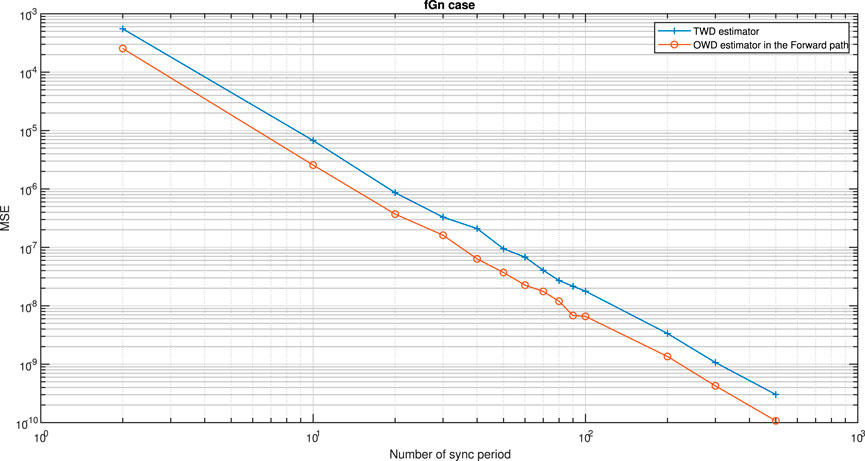
FIGURE 2. Test case a of Theorem 8. Performance (MSE) comparison between the OWD clock skew estimator in the Forward path (Eq. 61) and the TWD clock skew estimator (Eq. 60). The PDV is an fGn process. α = 50ppm, Q = 5 ms, $T_{syn}=15.6ms(64\frac{packet}{\sec })$, H = 0.7, d_ms = 5 ms, d_sm = 5.5 ms, ${\sigma }_{{\omega }_1}^2=4e-8[{\sec }^2]$, ${\sigma }_{{\omega }_2}^2=6.4e-7[{\sec }^2]$, Z = 16, ${\tilde{Z}}_{fGn/gfGn}(J=500)=3.233$ (for J < 500, ${\tilde{Z}}_{fGn/gfGn}<3.233$). The results were obtained for 100 Monte-Carlo trails.

FIGURE 3

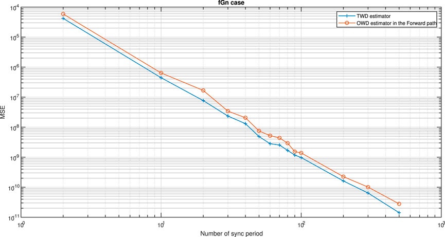
FIGURE 3. Test case a of Theorem 8. Performance (MSE) comparison between the OWD clock skew estimator in the Forward path (Eq. 61) and the TWD clock skew estimator (Eq. 60). The PDV is an fGn process. α = 50ppm, Q = 5 ms, $T_{syn}=15.6ms(64\frac{packet}{\sec })$, H = 0.7, d_ms = 5 ms, d_sm = 5.5 ms, ${\sigma }_{{\omega }_1}^2=1e-8[{\sec }^2]$, ${\sigma }_{{\omega }_2}^2=1.44e-8[{\sec }^2]$, Z = 1.44, ${\tilde{Z}}_{fGn/gfGn}(J=500)=3.058$ (for J < 500, ${\tilde{Z}}_{fGn/gfGn}<3.058$, ${\tilde{Z}}_{fGn/gfGn}(J=10)=3.004$). The results were obtained for 100 Monte-Carlo trails.

FIGURE 4

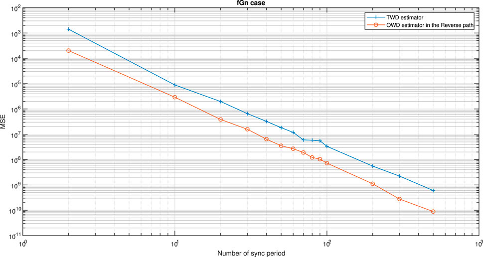
FIGURE 4. Test case b of Theorem 8. Performance (MSE) comparison between the OWD clock skew estimator in the Reverse path (Eq. 62) and the TWD clock skew estimator (Eq. 60). The PDV is an fGn process. α = 50ppm, Q = 5 ms, $T_{syn}=15.6ms(64\frac{packet}{\sec })$, H = 0.7, d_ms = 5 ms, d_sm = 5.5 ms, ${\sigma }_{{\omega }_1}^2=6.4e-7[{\sec }^2]$, ${\sigma }_{{\omega }_2}^2=4e-8[{\sec }^2]$, Z = 0.0625, ${\bar{Z}}_{fGn/gfGn}(J=500)=0.748$ (for J < 500, ${\bar{Z}}_{fGn/gfGn}<0.748$, ${\bar{Z}}_{fGn/gfGn}(J=10)=0.36$). The results were obtained for 100 Monte-Carlo trails.

FIGURE 5

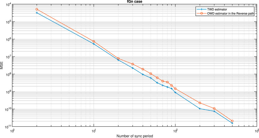
FIGURE 5. Test case b of Theorem 8. Performance (MSE) comparison between the OWD clock skew estimator in the Reverse path (Eq. 62) and the TWD clock skew estimator (Eq. 60). The PDV is an fGn process. α = 50ppm, Q = 5 ms, $T_{syn}=15.6ms(64\frac{packet}{\sec })$, H = 0.7, d_ms = 5 ms, d_sm = 5.5 ms, ${\sigma }_{{\omega }_1}^2=1.44e-8[{\sec }^2]$, ${\sigma }_{{\omega }_2}^2=1e-8[{\sec }^2]$, Z = 0.69, ${\bar{Z}}_{fGn/gfGn}(J=500)=0.3427$ (for J < 500, ${\bar{Z}}_{fGn/gfGn}<0.3427$). The results were obtained for 100 Monte-Carlo trails.

FIGURE 6

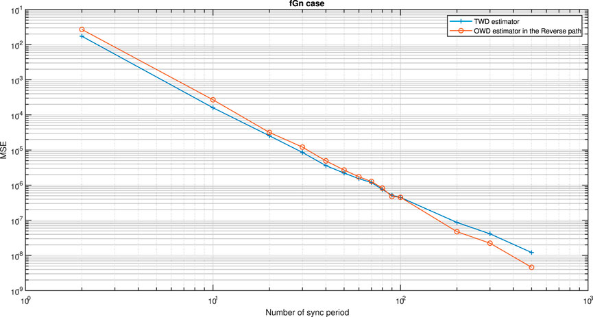
FIGURE 6. Test case c of Theorem 8. Performance (MSE) comparison between the OWD clock skew estimator in the Reverse path (Eq. 62) and the TWD clock skew estimator (Eq. 60). The PDV is an fGn process. α = 50ppm, Q = 5 ms, $T_{syn}=15.6ms(64\frac{packet}{\sec })$, H = 0.6, d_ms = 2.5 ms, d_sm = 3 ms, ${\sigma }_{{\omega }_1}^2={\sigma }_{{\omega }_2}^2=4e-6[{\sec }^2]$, Z = 1, ${\tilde{\sigma }}_{fGn/gfGn}^2(J=500)=1.03e-6$ (for J < 500: ${\tilde{\sigma }}_{fGn/gfGn}^2>1.03e-6$, ${\tilde{\sigma }}_{fGn/gfGn}^2(J=100)=3e-6$, ${\tilde{\sigma }}_{fGn/gfGn}^2(J=60)=4.3e-6$, ${\tilde{\sigma }}_{fGn/gfGn}^2(J=10)=1.72e-5$). The results were obtained for 100 Monte-Carlo trails.

FIGURE 7

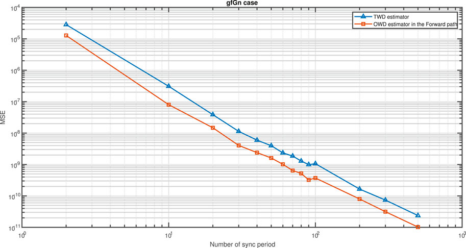
FIGURE 7. Test case a of Theorem 8. Performance (MSE) comparison between the OWD clock skew estimator in the Forward path (Eq. 61) and the TWD clock skew estimator (Eq. 60). The PDV is an gfGn process. α = 50ppm, Q = 5 ms, $T_{syn}=15.6ms(64\frac{packet}{\sec })$, H = 0.95, a = 0.08, d_ms = 5 ms, d_sm = 5.5 ms, ${\sigma }_{{\omega }_1}^2=1e-8[{\sec }^2]$, ${\sigma }_{{\omega }_2}^2=9e-8[{\sec }^2]$, Z = 9, ${\tilde{Z}}_{fGn/gfGn}(J=500)=3.02$ (for J < 500, ${\tilde{Z}}_{fGn/gfGn}<3.02$). The results were obtained for 100 Monte-Carlo trails.

FIGURE 8

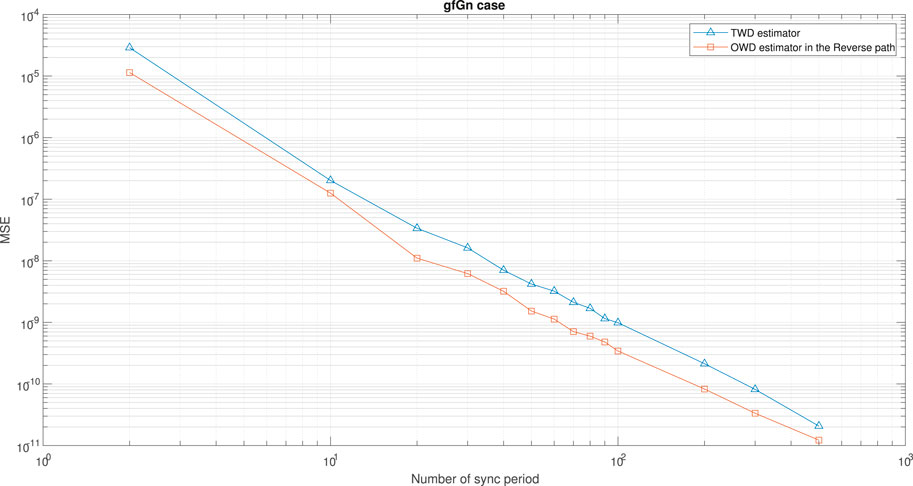
FIGURE 8. Test case b of Theorem 8. Performance (MSE) comparison between the OWD clock skew estimator in the Reverse path (Eq. 62) and the TWD clock skew estimator (Eq. 60). The PDV is an gfGn process. α = 50ppm, Q = 5 ms, $T_{syn}=15.6ms(64\frac{packet}{\sec })$, H = 0.95, a = 0.08, d_ms = 5 ms, d_sm = 5.5 ms, ${\sigma }_{{\omega }_1}^2=9e-8[{\sec }^2]$, ${\sigma }_{{\omega }_2}^2=1e-8[{\sec }^2]$, Z = 0.111, ${\bar{Z}}_{fGn/gfGn}(J=500)=0.356$ (for J < 500, ${\bar{Z}}_{fGn/gfGn}<0.356$, ${\bar{Z}}_{fGn/gfGn}(J=10)=0.337$). The results were obtained for 100 Monte-Carlo trails.

In Figures 9–12 we compared the clock skew performance (MSE) of our new proposed OWD clock skew estimators (Eqs 61, 62) with the clock skew performance (MSE) that is obtained from three clock skew algorithms: a.) TWD clock skew estimator, named as the ML-like estimator (MLLE) proposed by Noh et al. [5], b.) OWD clock skew estimator, named as the maximum likelihood estimator proposed by Levy and Pinchas [7], c.) OWD clock skew estimator, named as the Kalman estimator proposed by Chaloupka et al. [6]. According to Noh et al. [5] we have:

$\widehat{\beta }=\frac{T_{\mathrm{2,1}}{\left(J-1\right)}^2+T_{\mathrm{3,1}}{\left(J-1\right)}^2}{T_{\mathrm{1,1}}\left(J-1\right)T_{\mathrm{2,1}}\left(J-1\right)+T_{\mathrm{3,1}}\left(J-1\right)T_{\mathrm{4,1}}\left(J-1\right)}-1(101)$

where

$\widehat{\beta }=\frac{1}{\widehat{\alpha }+1}-1(102)$

T_2,1 (J − 1) = t₂ [J] − t₂ [1], T_1,j(i), T_2,j(i), T_3,j(i) and T_4,j(i) are defined in Eqs 4, 13.

FIGURE 9

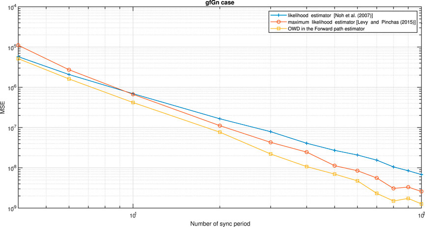
FIGURE 9. Performance (MSE) comparison between the OWD clock skew estimator for the Forward path (Eq. 61), likelihood clock skew estimator proposed by Noh et al. [5] and maximum likelihood clock skew estimator proposed by Levy and Pinchas [7]. The PDV is an gfGn process. α = 50ppm, Q = 5 ms, $T_{syn}=15.6ms(64\frac{packet}{\sec })$, H = 0.95, a = 0.08, d_ms = 5.5 ms, d_sm = 5 ms, ${\sigma }_{{\omega }_1}^2=4e-8[{\sec }^2]$, ${\sigma }_{{\omega }_2}^2=1.6e-7[{\sec }^2]$. The results were obtained for 100 Monte-Carlo trails.

FIGURE 10

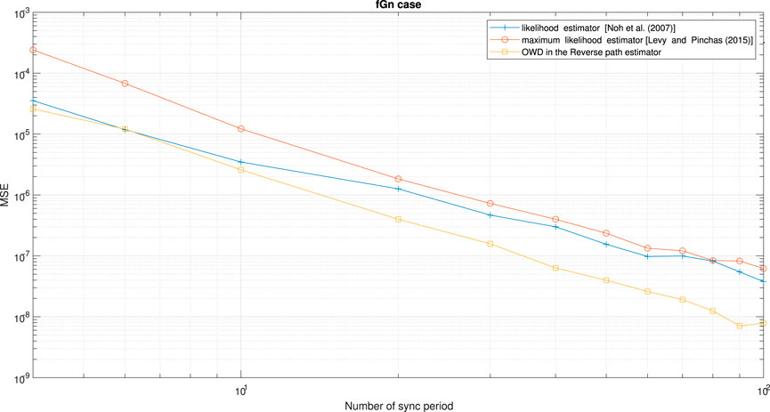
FIGURE 10. Performance (MSE) comparison between the OWD clock skew estimator for the Reverse path (Eq. 62), likelihood clock skew estimator proposed by Noh et al. [5] and maximum likelihood clock skew estimator proposed by Levy and Pinchas [7]. The PDV is an fGn process. α = 50ppm, Q = 5 ms, $T_{syn}=15.6ms(64\frac{packet}{\sec })$, H = 0.7, d_ms = 5.5 ms, d_sm = 5 ms, ${\sigma }_{{\omega }_1}^2=1.6e-7[{\sec }^2]$, ${\sigma }_{{\omega }_2}^2=4e-8[{\sec }^2]$. The results were obtained for 100 Monte-Carlo trails.

FIGURE 11

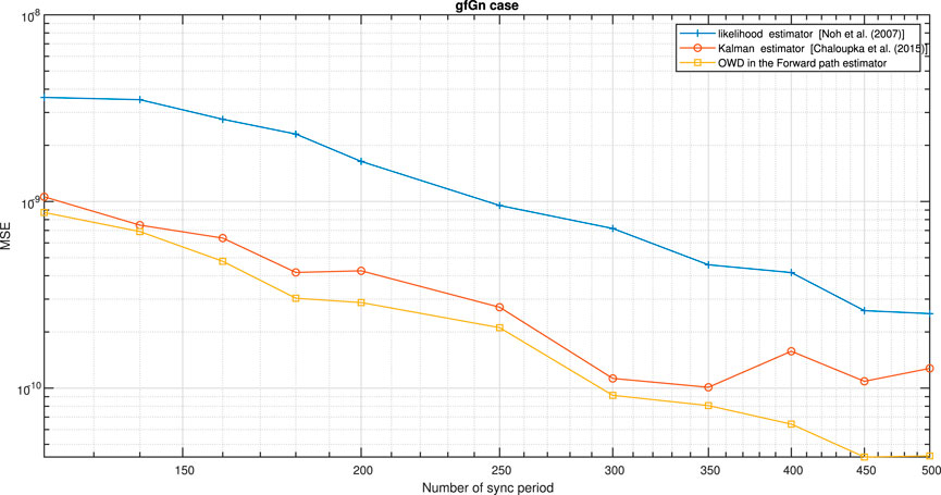
FIGURE 11. Performance (MSE) comparison between the OWD clock skew estimator for the Forward path (Eq. 61), likelihood clock skew estimator proposed by Noh et al. [5] and Kalman clock skew estimator proposed by Chaloupka et al. [6]. The PDV is an gfGn process. α = 50ppm, Q = 5 ms, $T_{syn}=15.6ms(64\frac{packet}{\sec })$, H = 0.95, a = 0.08, d_ms = 5.5 ms, d_sm = 5 ms, ${\sigma }_{{\omega }_1}^2=4e-8[{\sec }^2]$, ${\sigma }_{{\omega }_2}^2=1.3e-7[{\sec }^2]$, L = 100, Q_KAL = 0, δ_σ = δ_μ = 1e − 4, $\widehat{\mu }[1]=0$. The results were obtained for 100 Monte-Carlo trails.

FIGURE 12

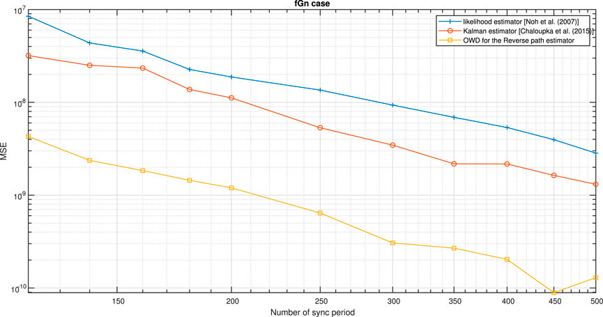
FIGURE 12. Performance (MSE) comparison between the OWD clock skew estimator for the Reverse path (Eq. 62), likelihood clock skew estimator proposed by Noh et al. [5] and Kalman clock skew estimator proposed by Chaloupka et al. [6]. The PDV is an fGn process. α = 50ppm, Q = 5 ms, $T_{syn}=15.6ms(64\frac{packet}{\sec })$, H = 0.7, d_ms = 5.5 ms, d_sm = 5 ms, ${\sigma }_{{\omega }_1}^2=3.6e-7[{\sec }^2]$, ${\sigma }_{{\omega }_2}^2=4e-8[{\sec }^2]$, L = 100, Q_KAL = 0, δ_σ = δ_μ = 1e − 4, $\widehat{\mu }[1]=0$. The results were obtained for 100 Monte-Carlo trails.

According to Levy and Pinchas [7] we have:

$\begin{array}{cc}\hfill \widehat{\epsilon }=& \left(2\sum _{i=1}^J\sum _{j=1}^J\sum _{k=1}^{\mathit{min}\left(i,j\right)-1}\left[A_{\mathit{max}}\left(J,i,j,k,H\right)\left(△T_{s1.i}-△T_{s2.i}\right)\left(△T_{s1.j}-△T_{s2.j}\right)\right]\right)\hfill \\ \hfill & \left(\sum _{i=1}^J\sum _{j=1}^J\sum _{k=1}^{\mathit{min}\left(i,j\right)-1}\left[A_{\mathit{max}}\left(J,i,j,k,H\right)\left[△T_{m.j}\left(△T_{s1.i}-△T_{s2.i}\right)\right.\right.\right.\hfill \\ \hfill & +{\left.\left.\left.△T_{m.i}\left(△T_{s1.j}-△T_{s2.j}\right)\right]\right]\right)}^{-1}-1\hfill \end{array}(103)$

where A_max (J, i, j, k, H) is:

$\begin{array}{cc}\hfill A_{\mathit{max}}& \left(J,i,j,k,H\right)={\left[\frac{\mathrm{\Gamma }\left(J\right)}{\mathrm{\Gamma }\left(-H+0.5\right)\mathrm{\Gamma }\left(J-H+0.5\right)}\right]}^2\left(\mathrm{\Gamma }\left(i-k-H+0.5\right)\right.\hfill \\ \hfill & \left.\mathrm{\Gamma }\left(J-H+0.5-i+k\right)\mathrm{\Gamma }\left(j-k-H+0.5\right)\mathrm{\Gamma }\left(J-H+0.5-j+k\right)\right)\hfill \\ \hfill & {\left(\mathrm{\Gamma }\left(J-i+k\right)\mathrm{\Gamma }\left(J-j+k\right)\mathrm{\Gamma }\left(i-k\right)\mathrm{\Gamma }\left(j-k\right)\right)}^{-1}\hfill \\ \hfill & \left[\frac{1}{\left(i-k\right)}\frac{1}{\left(j-k\right)}-\frac{1}{\left(J-i+k\right)}\frac{1}{\left(J-j+k\right)}\right]\hfill \end{array}(104)$

and $\widehat{\epsilon }$ is:

$\widehat{\epsilon }=\frac{1}{\widehat{\alpha }+1}-1(105)$

Γ(.) denotes the Gamma function, △ denotes the difference between two consecutive timestamps. T_{m. i} is the timestamp in the ith period when the Master sends the Sync message. T_{s1. i} is the timestamp in the ith period when the dual-Slave receives the Sync message. T_{s2. i} is the timestamp in the ith period when the Slave receives the Sync message.

The Kalman estimator from Chaloupka et al. [6] depends on a predefined parameter L that defines the sliding window’s length in the algorithm. The L parameter impacts the performance (MSE). As we increase L, it reduces the MSE. However, L also depends on the total number of sync periods, which we set for the frequency synchronization task as 500. Therefore, L must be smaller than 500.

According to Chaloupka et al. [6] the Kalman’s measurement equation is:

$T_{1,j}\left(L\right)-T_{2,j}\left(L\right)=T_{2,j}\left(L\right)\alpha \left[j\right]+{\mathrm{\Omega }}_{1,j}\left(L\right)(106)$

The Kalman’s state equation is:

$\widehat{\alpha }\left[j+1\right]=\widehat{\alpha }\left[j\right]+u\left[j\right].(107)$

where the variance of u[j] is Q_KAL. The estimate of the noise measurement variance is given by Chaloupka et al. [6]:

$\widehat{R}\left[j\right]=\left(1-{\delta }_{\sigma }\right)\widehat{R}\left[j-1\right]+{\delta }_{\sigma }{\left(x\left[j\right]-\widehat{\mu }\left[j\right]\right)}^2(108)$

where

$\widehat{\mu }\left[j\right]=\left(1-{\delta }_{\mu }\right)\widehat{\mu }\left[j-1\right]+{\delta }_{\mu }x\left[j\right];x\left[j\right]=T_{1,j}\left(L\right)-T_{2,j}\left(L\right)(109)$

δ_μ and δ_σ are smoothing factors which are between zero and one.

According to Figures 9, 10, our new proposed OWD clock skew estimator for the Forward path (Eq. 61) (Figure 9) or for the Reverse path (Eq. 62) (Figure 10) achieves a lower MSE compared to the clock skew estimators proposed by Noh et al. [5] and Levy and Pinchas [7]. Please note that for the simulation results presented in Figure 10, the PDV for the Reverse path was set lower than the PDV for the Forward path. Since the OWD clock skew estimator proposed by Levy and Pinchas [7] is based on the Forward path only, the clock skew accuracy with this estimator Levy and Pinchas [7] is indeed decreased (Figure 10).

According to Figures 11, 12, our new proposed OWD clock skew estimator for the Forward path (Eq. 61) (Figure 11) or for the Reverse path (Eq. 62) (Figure 12) achieves a lower MSE compared to the clock skew estimators proposed by Noh et al. [5] and Chaloupka et al. [6]. Please note that for the simulation results presented in Figure 12, the PDV for the Reverse path was set lower than the PDV for the Forward path. Since the OWD clock skew estimator proposed by Chaloupka et al. [6] is based on the Forward path only, the clock skew accuracy with this estimator Chaloupka et al. [6] is indeed decreased (Figure 12).

Next we tested our new proposed OWD clock skew estimators’ performances (MSE) for the Forward and Reverse paths (Eqs 61, 62) with our closed-form-approximated expressions for the MSE for the LRD case (Eqs 54, 58) for the Forward and Reverse path, respectively. Case 1 in Figures 13, 14 presents the clock skew performance of our new proposed OWD clock skew estimator for the Forward path (Eq. 61) compared with our closed-form-approximated expression for the MSE in Eq. 54. Case 2 in Figures 13, 14 presents the clock skew performance of our new proposed OWD clock skew estimator for the Reverse path (Eq. 62) compared with our closed-form-approximated expression for the MSE in Eq. 58. According to Figures 13, 14 it can be clearly seen that our new closed-form-approximated expressions for the MSE in Eqs 54, 58 supply very close results to the simulated one.

FIGURE 13

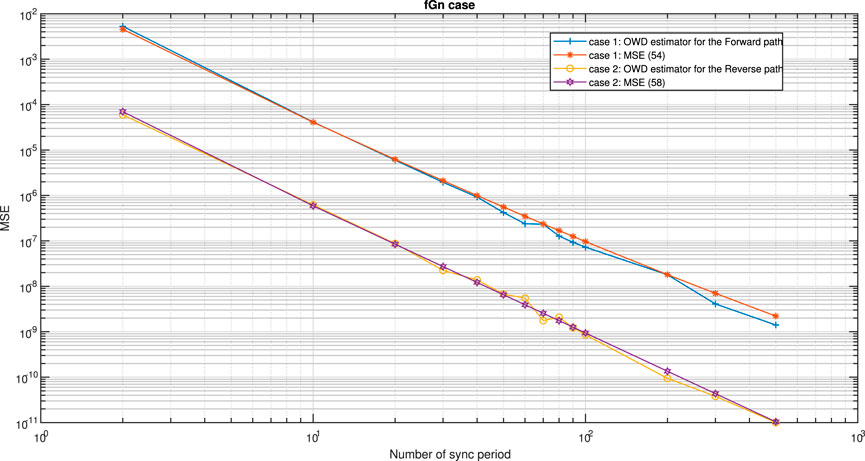
FIGURE 13. case 1: Performance comparison for the fGn case, between our new proposed clock skew estimator for the Forward path (Eq. 61) with the performance results for our new proposed expression for the MSE (Eq. 54). ${\sigma }_{{\omega }_1}=0.8e-3[\sec ]$. Case 2: Performance comparison for the fGn case, between our new proposed clock skew estimator for the Reverse path (Eq. 62) with the performance results for our new proposed expression for the MSE (Eq. 58). ${\sigma }_{{\omega }_2}=0.1e-3[\sec ]$. For both cases: α = 50ppm, Q = 5 ms, $T_{syn}=15.6ms(64\frac{packet}{\sec })$, H = 0.6, d_ms = 5.5 ms, d_sm = 5 ms. The results were obtained for 100 Monte-Carlo trails.

FIGURE 14

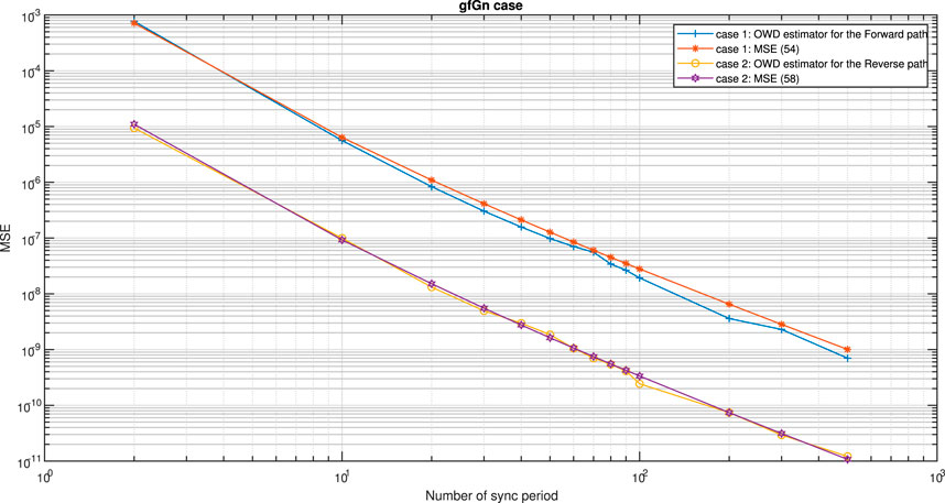
FIGURE 14. case 1: Performance comparison for the gfGn case, between our new proposed clock skew estimator for the Forward path (Eq. 61) with the performance results for our new proposed expression for the MSE (Eq. 54). ${\sigma }_{{\omega }_1}=0.8e-3[\sec ]$. Case 2: Performance comparison for the gfGn case, between our new proposed clock skew estimator for the Reverse path (Eq. 62) with the performance results for our new proposed expression for the MSE (Eq. 58). ${\sigma }_{{\omega }_2}=0.1e-3[\sec ]$. For both cases: α = 50ppm, Q = 5 ms, $T_{syn}=15.6ms(64\frac{packet}{\sec })$, H = 0.95, a = 0.95, d_ms = 5.5 ms, d_sm = 5 ms. The results were obtained for 100 Monte-Carlo trails.

8 Conclusion

In this paper we derived two novels OWD clock skew estimators for the Forward and Reverse paths applicable for white-Gaussian process and for the fGn/gfGn environment. Those estimators do not depend on the unknown fixed paths nor on the clock offset between the Master and Slave. In addition, we derived also closed-form-approximated expressions for the clock skew performance (MSE) for the new proposed OWD clock skew estimators for the Forward and Reverse paths. In order to help the system designer to choose the right clock skew estimator that may get the best clock skew performance from the MSE point of view, some guidelines (conditions) were derived, helping choosing the right clock skew estimator wisely. Simulation results has confirmed that our new OWD clock skew estimators indeed achieve better clock skew performance from the MSE point of view compared to the literature known clock skew estimators. Simulation results have also confirmed that our closed-form-approximated expressions for the MSE related to our new proposed OWD Forward and Reverse estimators are indeed efficient.

Data Availability Statement

The original contributions presented in the study are included in the article/Supplementary Material, further inquiries can be directed to the corresponding author.

Author Contributions

All authors listed have made a substantial, direct, and intellectual contribution to the work and approved it for publication.

Conflict of Interest

The authors declare that the research was conducted in the absence of any commercial or financial relationships that could be construed as a potential conflict of interest.

Publisher’s Note

All claims expressed in this article are solely those of the authors and do not necessarily represent those of their affiliated organizations, or those of the publisher, the editors, and the reviewers. Any product that may be evaluated in this article, or claim that may be made by its manufacturer, is not guaranteed or endorsed by the publisher.

References

1.[Dataset] Arnold D. IEEE 1588-2019-IEEE Standard for a Precision Clock Synchronization Protocol for Networked Measurement and Control Systems (2019). Available from: https://standards.ieee.org/standard/1588-2019.html (Accessed June 17, 2021).

2. K.Karthik A, S.Blum R. Estimation Theory Based Robust Phase Offset Estimation in the Presence of Delay Attacks (2016). Available from: https://arxiv.org/pdf/1611.05117.pdf (Accessed August 10, 2021).

3. Guruswamy A, Blum RS, Kishore S, Bordogna M. On the Optimum Design of L-Estimators for Phase Offset Estimation in IEEE 1588. IEEE Trans Commun (2015) 63:5101–15. doi:10.1109/TCOMM.2015.2493534

4. Avraham Y, Pinchas M. A Novel Clock Skew Estimator and its Performance for the IEEE 1588v2 (PTP) Case in Fractional Gaussian Noise/Generalized Fractional Gaussian Noise Environment. Front Phys (2021) 9:1–21. doi:10.3389/fphy.2021.796811

5. Noh K-L, Chaudhari QM, Serpedin E, Suter BW. Novel Clock Phase Offset and Skew Estimation Using Two-Way Timing Message Exchanges for Wireless Sensor Networks. IEEE Trans Commun (2007) 55:766–77. doi:10.1109/TCOMM.2007.894102

6. Chaloupka Z, Alsindi N, Aweya J. Clock Skew Estimation Using Kalman Filter and IEEE 1588v2 PTP for Telecom Networks. IEEE Commun Lett (2015) 19:1181–4. doi:10.1109/LCOMM.2015.2427158

7. Levy C, Pinchas M. Maximum Likelihood Estimation of Clock Skew in IEEE 1588 with Fractional Gaussian Noise. Math Probl Eng (2015) 2015:1. doi:10.1155/2015/174289

8. Karthik AK, Blum RS. Robust Clock Skew and Offset Estimation for IEEE 1588 in the Presence of Unexpected Deterministic Path Delay Asymmetries. IEEE Trans Commun (2020) 68:5102–19. doi:10.1109/TCOMM.2020.2991212

9. Karthik AK, Blum RS. Robust Phase Offset Estimation for IEEE 1588 PTP in Electrical Grid Networks. In: 2018 IEEE Power & Energy Society General Meeting (2018). doi:10.1109/PESGM.2018.8586488

10. Karthik AK, Blum RS. Optimum Full Information, Unlimited Complexity, Invariant, and Minimax Clock Skew and Offset Estimators for IEEE 1588. IEEE Trans Commun (2019) 67:3624–37. doi:10.1109/TCOMM.2019.2900317

11. Li M, Zhao W. On Bandlimitedness and Lag-Limitedness of Fractional Gaussian Noise. Physica A: Stat Mech its Appl (2013) 392:1955–61. doi:10.1016/j.physa.2012.12.035

12. Cappe O, Moulines E, Pesquet J-C, Petropulu AP, Xueshi Y. Long-range Dependence and Heavy-Tail Modeling for Teletraffic Data. IEEE Signal Process Mag (2002) 19:14–27. doi:10.1109/79.998079

13. Li M. Generalized Fractional Gaussian Noise and its Application to Traffic Modeling. Physica A: Stat Mech its Appl (2021) 579:126138. doi:10.1016/j.physa.2021.126138