 Helena Yoest 1†John Buggeln 1†
 Minh Doan 1†Payton Johnson 1†
 Simon A. Berman2
 Kevin A. Mitchell 2
 Thomas H. Solomon 1*
- 1Department of Physics and Astronomy, Bucknell University, Lewisburg, PA, United States
- 2Department of Physics, University of California, Merced, Merced, CA, United States
We present experiments on the motion of swimming microbes in a laminar, hyperbolic flow. We test a theory that predicts the existence of swimming invariant manifolds (SwIMs) that act as invisible, one-way barriers that block the motion of the microbes. The flow is generated in a cross-channel in a PDMS cell, driven by syringe pumps. The swimming microbes are euglena and tetraselmis, both single-celled, eukaryotic algae. The algae are not ideal smooth-swimmers: there is significant rocking in their motion with occasional tumbles and a swimming speed that can vary. The experiments show that the swimming algae are bound very effectively by the predicted SwIMs. The different shapes and swimming behavior of the euglena and tetraselmis affect the distribution of swimming angles, with the elongated euglena having a larger probability of swimming in a direction parallel to the outflow directions. The differences in swimming orientation affect the ability of the microbes to penetrate the manifolds that act as barriers to passive tracers. The differing shapes of the euglena and tetraselmis also affect probabilities for the microbes to escape in one direction or the other along the outflow.
1 Introduction
In the 1980s and 1990s, the tools of dynamical systems and chaos theory were applied to developing an understanding of fluid mixing in laminar flows [1, 2]. In particular, manifolds were identified [3–5] that were found to act as barriers that block the motion and mixing of impurities in a wide range of laminar flows. Furthermore, lobes (or “turnstiles”) formed from these manifolds were found to explain long-range transport in flows with simple periodic time dependence [6–8]. These dynamical tools have been extended to identify local barriers and “Lagrangian coherent structures” that guide and organize transport and mixing in spatially- and temporally-complicated fluid flows [9–14]. These results have led to a range of applications in diverse physical systems such as the spread of pollution in the oceans and atmosphere [12, 15], transport barriers in nuclear fusion plasmas [16], blood transport in cardiovascular flows [17] and morphogenesis in developing embryos [18].
For most of these studies, mixing is passive, characterized by impurities that simply follow a flow without any deviations and without any influence on the flow itself. But mixing in real systems is often active, involving impurities that deviate from the flow and/or impurities that feed back and alter the flow. The behavior of propagating reaction fronts in a fluid flow is an example of active mixing, since the reaction fronts are able to move across a fluid even in the absence of flows. The theory of manifolds developed for passive mixing has been extended to the problem of front propagation in fluid flows [19, 20]. In this case, burning invariant manifolds (BIMs) permeate the fluid system and act as one-way barriers that both hinder and guide the behavior of fronts in a wide range of fluid flows. We have done numerous experiments that have demonstrated the role of BIMs as one-way barriers in a wide range of two-dimensional [21–23] and three-dimensional laminar fluid flows [24].
Another class of active impurities are those that are self-propelled, such as biological organisms ranging from bacteria [25–28] to birds and people [29], and artificial swimmers ranging from microscopic Janus particles [30–32] to ships. A modified and extended version of the burning invariant manifold theory [33, 34] predicts similar manifolds—referred to as swimming invariant manifolds (SwIMs)—that act as barriers that inhibit and organize the mixing of self-propelled tracers in a flow. Edges of SwIMs act as one-way barriers when projected into (x, y) position space, similar to the one-way blocking of BIMs of reaction fronts in (x, y). In fact, the burning invariant manifold theory is a special case of the more general swimming invariant manifold approach. We have previously tested parts of this theory experimentally in a hyperbolic flow with rod-shaped, prokaryotic swimming bacteria, some of which were genetically mutated to inhibit tumbling [33].
In this paper, we present the results from additional experiments that test the applicability of SwIM theory to larger, less idealized swimmers with different shapes (both rod-shaped and circular) and different swimming behavior. We choose one of the simplest, non-trivial flows: a laminar, hyperbolic fluid flow in a cross channel. The hyperbolic flow is particularly special since the vorticity is zero everywhere. The self-propelled particles are two different types of eukaryotic swimming algae—freshwater algae (euglena) and marine algae (tetraselmis) that are both an order of magnitude larger in size than the prokaryotic bacteria studied earlier. We examine trajectories of these swimming microbes in the flow to see if they are bounded by the one-way barriers that are predicted by the SwIM theory. We also analyze orientation and escape probabilities in the context of the SwIM theory.
In Section 2, we present background about dynamical systems theory of manifolds as applied to the mixing of passive and self-propelled tracers. We discuss the experimental methods used to generate the hyperbolic fluid flow in Section 3, along with the techniques used for handling the microbes. Trajectories of the microbes in the flow are presented in Section 4, highlighting the SwIMs that act as barriers that impede their motion. We also present a statistical analysis of trajectories through (x, y, θ) phase space and orientation distributions in Section 4, interpreted using the SwIM framework. In Section 5 we discuss these results, as well as continuing work that is needed to further explore the range of applicability of SwIM theory for active mixing.
2 Background
2.1 Passive Mixing
The motion of passive tracers in a fluid flow is governed by the differential equations
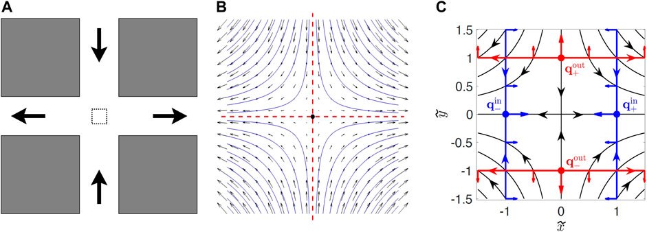
FIGURE 1. (A) Sketch of the PDMS cross-channel cell. Fluid is pumped in at the top and bottom and pumped out at the left and right. The dashed box in the middle of the intersection is the region where the flow is approximately hyperbolic. (B) Zoom in of flow in the dashed box in (A). The vertical (horizontal) red dashed line is the stable (unstable) passive manifold of the passive fixed point (dot at center). (C) Diagram showing swimming fixed points qin and qout, and swimming invariant manifolds (SwIM edges) in red and blue (from Ref. [34]). The red and blue arrows perpendicular to the SwIM edges in (C) show the swimming direction that is blocked by these structures.
There is a passive fixed point at (x, y) = (0, 0) where ux and uy are both zero (Figure 1B). Attached to this fixed point are two passive invariant manifolds. The unstable manifold of the fixed point is defined by starting with an infinite number of passive tracers initially located infinitesimally close to the fixed point and allowed to evolve in time. In the long-time limit, the locations to where those tracers have moved define the unstable manifold which, for a time-independent, hyperbolic flow is the line y = 0 (horizontal, red dashed line in Figure 1B). Similarly, the stable manifold of the fixed point is defined using the same approach, but integrating the trajectories backward in time. Alternately, the stable manifold is the locus of points that ultimately will end up infinitesimally close to the fixed point. For the hyperbolic flow of Eq. 1a, Eq. 1b, the stable manifold of the fixed point is the line x = 0 (vertical, red dashed line). The passive stable and unstable manifolds act as transport barriers for passive mixing. For the time-independent hyperbolic flow of Figure 1, the stable and unstable manifolds divide the flow into four quadrants, and passive tracers initially in one quadrant remain in that quadrant. For a time-independent flow, the identification of manifolds as transport barriers for passive mixing is a somewhat trivial result since passive tracers do not deviate from the streamlines in the flow. But the nature of manifolds as barriers persists to the less-trivial case of flows with periodic time-dependence [8, 35]. Studies during the past two decades have extended the ideas of manifolds as barriers to aperiodic and even turbulent flows, typical of flows in the oceans and atmospheres [9–14].
2.2 Self-Propelled Tracers
An example of a tracer that is not passive is one that is self-propelled such as a biological organism (e.g., swimming microbes, birds, people), synthetic microscale swimmers such as Janus particles [30–32], and larger-scale devices (e.g., cars, boats, drones, planes). In many cases, the self-propelled tracer is itself subject to flows in the surrounding medium; e.g., fish in a river, bacteria in the lungs or bloodstream, ships on the ocean.
Figure 2 shows an ellipsoidal swimmer. The aspect ratio γ = l‖/l⊥ is the ratio of the long and short dimensions of the ellipsoid, with l‖ defined parallel to the swimming direction. We assume a two dimensional flow, and assume that the self-propelled tracer swims at a constant speed V0 relative to the fluid without any noise or internally-imposed change in swimming direction (e.g., tumbling for a microbe). With these assumptions, the motion of the tracer is described by the following set of differential equations [36, 37, 38, 33]:
where (x, y) are the coordinates of the tracer, θ is the angle of the tracer’s swimming relative to the horizontal, and ω = uy,x − ux,y is the vorticity of the flow. The parameter α = (γ2 − 1)/(γ2 + 1) denotes the shape and swimming direction of the swimmer (Figure 2). Eq. 2a, Eq. 2b, Eq. 2c assume that the motion of the swimmers does not alter the fluid flow.
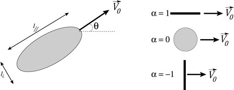
FIGURE 2. Sketch of ellipsoidal swimmer with labelled dimensions and special cases for swimmers with α = 1, 0 and −1.
For the zero-vorticity hyperbolic flow Eq. 1a, Eq. 1b, Eq. 2a, Eq. 2b, Eq. 2c simplify [33]:
If the self-propelled tracer swims smoothly with no internally-driven changes in swimming direction or external noise, there is no mechanism for the swimmer to rotate through angles θ = 0, π/2, π or 3π/2. In fact, swimming orientations of θ = 0 and π are stable attractors for any tracer with positive α, and swimming orientations of θ = π/2 and 3π/2 are stable for swimmers with negative α.
We can rewrite Eq. 3a, Eq. 3b, Eq. 3c in non-dimensional form by scaling distances by the distance V0/A and scaling time by A. Dimensionless coordinates are then defined as
With these definitions, dimensionless versions of Eq. 3a, Eq. 3b, Eq. 3c are:
There are swimming fixed points of Eq. 5 where

FIGURE 3. Manifolds in
Projections (called “SwIM edges”) of the edges of the SwIMs into physical
However, if a swimmer moves inward along the y-axis, the red SwIM edge along its path no longer blocks the swimmer, since the direction of the flow and the swimming are the same. The red SwIM edges are one-way barriers, blocking outward—but not inward—swimming tracers. Similarly, the blue swimming fixed points at
One-dimensional swimming invariant manifolds for α = −1 (which coincide with BIMs that block reaction fronts in the same flow) have been shown theoretically [34] to block all swimmers, even those that tumble or have rotational diffusion or added rotational noise, as long as their swimming speed remains constant. The location of the swimming fixed points and SwIM edges are independent of α for the hyperbolic flow and coincide with the BIMs. Consequently, the SwIM edges in the hyperbolic flow are predicted theoretically to be barriers even for tumbling swimmers.
3 Experimental Methods
3.1 Microbes
The microbes (Figure 4) used in these studies are two types of motile algae—euglena and tetraselmis. Euglena gracilis (Figure 4A) are freshwater algae that measure approximately 40–50 μm in length with a width of around 8–12 μm with aspect ratios γ ∼ 3–5 and α ∼ 0.8–0.9. (The euglena are not rigid and occasionally undulate in shape.) The euglena are propelled by a trailing flagellum that push the body forward. Tetraselmis (Figure 4D) are green marine algae that are almost circular with a typical diameter 10–15 μm; we estimate α to be approximately 0.3–0.4. Tetraselmis are pullers with four flagella at the front that beat in a breast-stroke pattern to pull the body forward.
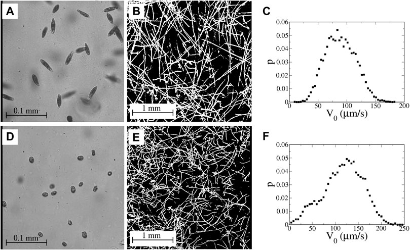
FIGURE 4. (A) Image of euglena, viewed at 40X magnification with a field of view of 320 μm. (B) Streak image showing motion of the euglena in the channel with no imposed flow; 4X magnification (3 mm field of view). (C) Measured probability distribution function (PDF) of speeds of swimming euglena in the absence of an imposed flow. (D) Image of tetraselmis, viewed at 40X magnification. (E) Motion of tetraselmis with no imposed flow; 4X magnification. (F) PDF of speeds of tetraselmis in the absence of an imposed flow. (Movies corresponding to the images in (B) and (E) are available online in Supplementary Material).
The estimates of α for both euglena and tetraselmis are crude. First, neither of them are perfect ellipsoids. Second, the shape varies from one organism to the next, especially for the euglena which are not even rigid. Furthermore, we neglect any effects of the extended flagella on α. But the difference in α is quite significant between the two organisms, with euglena being a reasonable approximation of an organism with α ≈ 1 and tetraselmis being a reasonable approximation of an organism with α ≈ 0.
The euglena and tetraselmis used in these experiments are standard, commercially-available samples obtained from Carolina Biological Supply without any effort at purifying the strain. The euglena are stored in the shipping tubes with continuous fluorescent illumination. Even a few months after shipment, euglena stored in this manner still swim actively. For use in an experimental run, the euglena samples from these tubes are diluted in soil-water medium (Carolina Biological Supply catalog #153785) at a concentration of 15–20% euglena sample by volume. For the tetraselmis, portions of the sample obtained from Carolina are cultured in Alga-Gro® Seawater medium (catalog #FAM_153754) with stirring and fluorescent illumination for 2 weeks, then transferred to 12 ml centrifuge tubes. Samples from these tubes are then diluted 1:1 with fresh Alga-Gro Seawater immediately before each experimental run.
3.2 PDMS Cells, Flow Generation and Measurement
The experiments are conducted in cross-channel cells (Figure 1) made from polydimethylsiloxane (PDMS); the channels are 4.0 mm wide and 2.0 mm deep. The flow is produced with two syringe pumps, one with two syringes attached via tubing to inlets/outlets at the top and bottom of the cross, and a second syringe pump with two syringes connected to inlets/outlets at the left and right ends of the cross. For a particular run, one syringe pump infuses fluid from two 1-ml syringes into the cell while the other syringe pump withdraws fluid at the same flow rate. The cell is mounted on an inverted microscope and imaged with a 4X objective. With this magnification, the visible region at the intersection of the two channels in the cross has a width and height of 3 mm.
For velocimetry measurements, 5.0 μm dyed (blue) polystyrene microspheres are used as passive tracers. In all experiments (both with passive and with swimming particles), the tracers are imaged only in a region near the mid-height of the cell to avoid slow-down in the flow due to the no-slip boundary conditions at the top and bottom.
Images are acquired using a CCD video camera. A background image determined by averaging frames over several seconds is subtracted from each image, and the resulting image is thresholded. These thresholded images are analyzed in IDL with a package developed by John Crocker and Eric Weeks [39] that determines centroid coordinates for clusters of pixels (with each cluster identified as a tracer), and then links coordinates in successive frames to determine trajectories. For the passive tracers, these trajectories are then used to determine local velocities. With a sufficient density, a velocity field is constructed, as shown in Figure 5A. (The region of interest is not centered on the flow, but that has no bearing on the analysis.) Linear regressions of slices of this velocity (Figure 5B) are used to determine the parameter A that denotes the strength of the velocity field of Eq. 1a, Eq. 1b. Deviations of the experimental velocity field from a true hyperbolic flow are shown in Figure 5C. Not surprisingly, the linear growth in the velocity is limited to a finite distance from the fixed point, since the fluid velocity has a finite peak at the inlet and outlet channels. This shows up in Figure 5C by the difference vectors which are opposite the flow far from the fixed point.
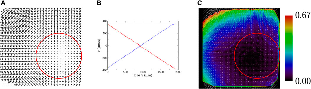
FIGURE 5. (A) Experimental velocity field, determined with passive tracers; flow rate 200 μl/min, A = 3.6 s−1. The red circle shows the region of interest used for all of the statistical analyses of microbe data. (B) Slices of the velocity field; ux along a horizontal line through the fixed point (blue), and uy along a vertical line through the fixed point (red). These curves are fit to a line to determine A in Eq. 1a, Eq. 1b. (C) Vector field showing the deviation of the experimentally-measured velocity field from an ideal hyperbolic velocity field Eq. 1a, Eq. 1b; i.e.,
For runs with swimming microbes, we fit x − and y − components of the trajectories separately to sliding parabolas and take derivatives to determine the x − and y − components of the total velocity of the trajectory
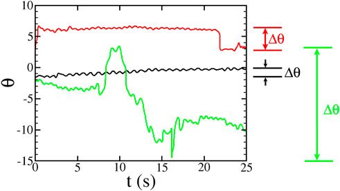
FIGURE 6. : Sample plots of swimming orientation θ for three microbes in the hyperbolic flow with A = 1.8 s−1 (flow rate 0.100 ml/min). Δθ is the largest angular difference between any two points in the trajectory. The red and green trajectories have |Δθ| > π and are labelled as “tumblers” whereas the black trajectory with |Δθ| < π is labelled a “non-tumbler.” The rocking motion of the swimming can be seen as oscillations in these plots.
A series of experimental runs for swimming microbes is obtained using the following protocol. After loading the tubing and PDMS cell with microbe-laden fluid, 1 ml syringes are loaded with new fluid and then data is taken with the flow in the “forward” direction (fluid pumped in along the vertical channel and out along the sides). After 1.0 ml of fluid is pumped (the capacity of the syringe), the flow is stopped. Data is then taken for a minute or two of the microbes swimming without a flow. The flow is then reversed and data is taken with the fluid pumped in along the horizontal and out along the vertical. Another no-flow run is taken at the end of the “reverse” run, after which another forward run is obtained. This process of forward/no-flow/reverse/no-flow/forward/no-flow … continues for 2–3 h for each set of data or until the microbe swimming is diminished.
4 Results
4.1 No Flow
The euglena used in these studies swim fairly smoothly with only occasional tumbling. Even in the absence of tumbling, though, there is still variation in the swimming direction due to rocking back and forth in the swimming (a two-dimensional projection of helical swimming) and noise in the swimming behavior. Figure 4B shows a streak image of euglena swimming in the cross-channel cell with no imposed flow. (Movies of this are available online in Supplementary Material) Close inspection of some of the streaks in Figure 4B shows periodic wiggling due to the rocking motion. Virtually every euglena remains motile throughout the course of a sequence of experiments, which continue for 2–3 h.
The swimming behavior of the tetraselmis is more varied. Not all of the tetraselmis in a sample are motile; during any run, some of the tetraselmis remain sessile with the fraction of sessile microbes increasing over the course of a sequence of experimental runs. A streak image of tetraselmis in the channel with no flow is shown in Figure 4E. Similar to the euglena, some of the tetraselmis tumble noticeably and others swim more smoothly, although there is clear rocking (wiggling of some of the trajectories in Figure 4E) and noise in the orientations even for the tetraselmis that are not undergoing classic run-and-tumble motion.
Probability distributions of average swimming speeds in the absence of a flow are shown for euglena and tetraselmis in Figures 4C,F, respectively. (For the tetraselmis data in Figure 4F, the sessile microbes are excluded.). The mean swimming speed (with no flow) is 90 and 120 μm/s for the euglena and tetraselmis, respectively. (The imposed flows in these experiments have no significant measurable effect on these mean swimming speeds.) Unlike the bacteria in the previous study [33], the swimming speed for an individual microbe is not necessarily constant in time. In fact, when tetraselmis tumble, they slow down to a stop before changing orientation.
4.2 Euglena in Hyperbolic Flow
A streak image of euglena moving in the hyperbolic flow is shown in Figure 7A. (A movie of the euglena swimming in the same flow can be found in online Supplementary Material) The effects of the swimming on the motion are clear in this figure, signified by frequent crossing of the trajectories. As can be seen in the movie and the plot of the orientation for a typical non-tumbling microbe (black curve in Figure 6), there is a strong preference for the euglena to be oriented horizontally (θ = 0 or π radians), particularly near the unstable passive manifold of the flow’s fixed point. This is consistent with Eq. 3c, which indicates that
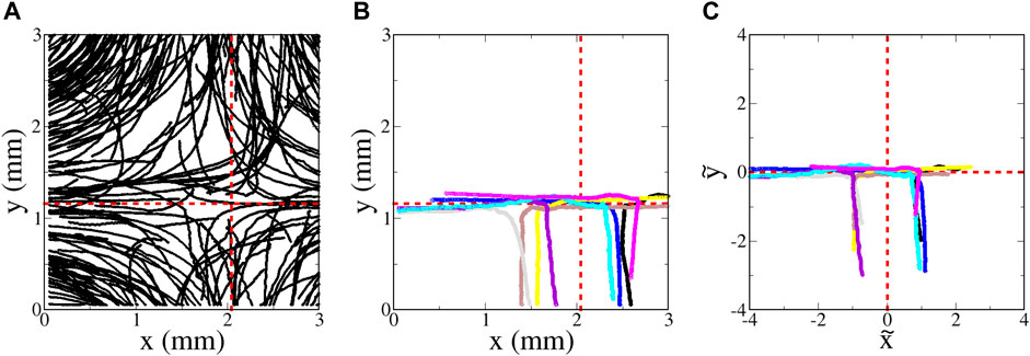
FIGURE 7. Euglena swimming in a hyperbolic flow with A = 1.8 s−1 (flow rate 0.100 ml/min). (A movie showing the motion of the euglena can be found online with Supplementary Material) (A) Random sampling of a very small subset of the trajectories. (B) Sampling of eight of the longest-duration trajectories with minimal tumbling that entered the region from the bottom. (C) Same as (B), but plotted using non-dimensional variables
Figure 6 shows the swimming orientation θ for three different types of trajectories observed in these experiments. Non-tumbling (“smooth”) trajectories often look like the black curve in Figure 6. There are two ways in which a tracer can show tumbling behavior. In some cases, similar to the red curve in Figure 6, the swimming is mostly smooth, with occasional and well-defined tumbling events where the orientation θ quickly changes. In many cases, though, the tumbling is more continuous, similar to the green curve in Figure 6. For the rest of the data analysis, we consider only the trajectories that are classified as non-tumbling.
Figure 7B shows a small sampling of trajectories determined by tracking the euglena; this figure shows the longest-duration, tracked, non-tumbling trajectories that initially enter from the bottom. It is difficult to interpret this plot vis-a-vis SwIM theory; since different euglena microbes swim with different average speed ⟨V0⟩, the location of the swimming fixed points and manifolds differ between each of the trajectories. To compare the trajectories with the swimming invariant manifold theory, we need to take into account the fact that each microbe has a different swimming speed. We use the dimensionless coordinates
The blocking behavior of the SwIMs can be seen by plotting the trajectories in groupings sorted by the directions from which they enter and to which they leave the hyperbolic flow region. Figure 8A shows all of the microbes that enter from the top and depart the hyperbolic flow to the left. Virtually none of these trajectories appear at any point to the right of the inward-blocking SwIM edge at
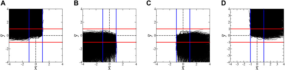
FIGURE 8. Trajectories of euglena in hyperbolic flow with A = 1.8 s−1. (These data exclude trajectories with classic run-and-tumble events during a trajectory.) The blue and red lines show the inward- and outward-blocking SwIM edges, respectively. (A) All trajectories that enter from the top and leave to the left. (B) All trajectories that enter from the bottom and leave to the left. (C) All trajectories that enter from the bottom and leave to the right. (D) All trajectories that enter from the top and leave to the right.
In earlier studies with bacteria [33] (and with more than an order of magnitude fewer trajectories), the barriers due to the SwIM edges at
For instance, since right-facing microbes move more slowly near the
Plots of pleft for euglena are shown in Figure 9A. Theoretically, any microbe with
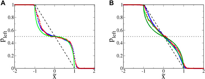
FIGURE 9. : Probability pleft for swimming microbes to move leftward, given a starting location
The slight leakage of the SwIMs as one-way barriers can be understood by considering the swimming speeds. Unlike the bacteria studied previously [33], the euglena do not always swim at a constant speed. The speed ⟨V0⟩ used to non-dimensionalize the coordinates is an average of the swimming speed during a trajectory. If the microbe is momentarily swimming with a speed larger than ⟨V0⟩, it can cross over what would be the barrier for a microbe swimming at the lower average speed.
The functional form of
Looking again at Figure 8, there is very little penetration of the euglena past the horizontal passive manifold at
We make a 3D histogram in
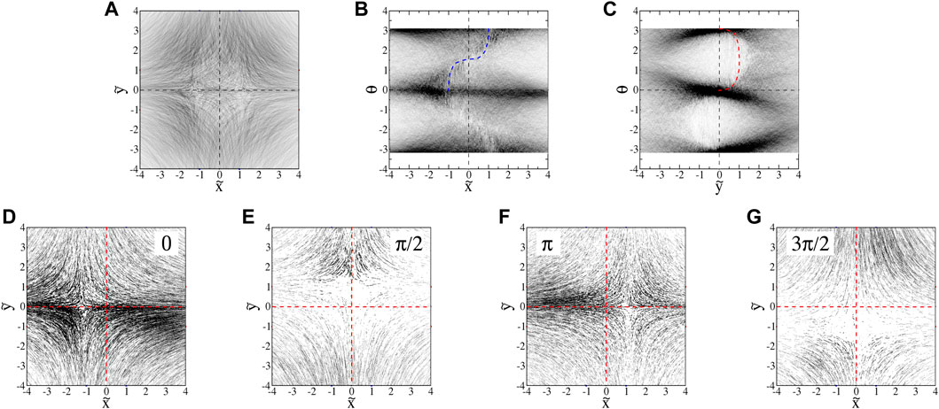
FIGURE 10. : Projections of euglena histograms (0.200 ml/min flow, A = 3.6s−1) into (A)
There are significant density variations in the
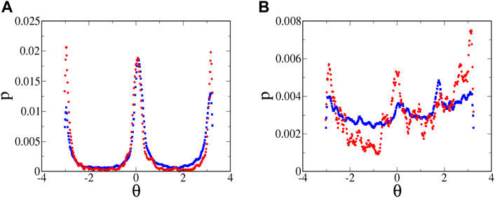
FIGURE 11. Probability distribution of swimming angles for microbes at
The distributions in Figure 11A cannot be compared quantitatively with the theoretical predictions for orientation distributions in Ref. [34]. The theoretical predictions assume a flow that is hyperbolic over an infinite extent, which is clearly not the case for the experiments. (In fact, there are even deviations within the field of view of the camera, as seen in Figure 5C.) In the experiments, the fluid and microbes are pumped through long tubes and then through channels leading to the intersection of the cross, and only in this intersection is the flow well approximated as hyperbolic. Furthermore, in the theoretical predictions, the distribution is calculated over all values of
Slices of the
4.3 Tetraselmis in Hyperbolic Flow
Trajectories of tetraselmis swimming in a hyperbolic flow are shown in Figure 12. These plots do not include the sessile microbes (determined by a threshold in measured ⟨V0⟩); we also exclude trajectories that are undergoing classic run-and-tumble behavior (determined again by examining differences in orientation Δθ). Once again, we plot the longest-duration trajectories in Figure 12B,C
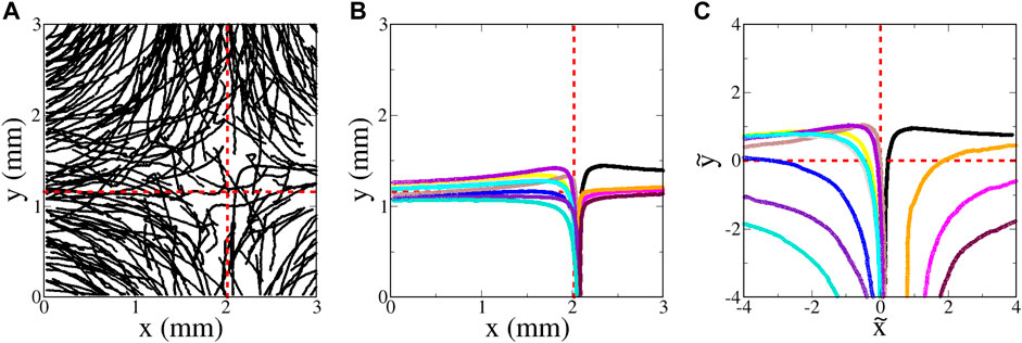
FIGURE 12. Tetraselmis swimming in a hyperbolic flow with A = 3.6 s−1 (flow 0.100 ml/min). (A) Random sampling of a very small subset of the trajectories. (B) Sampling of twelve of the longest-duration trajectories with minimal tumbling that entered from the bottom. (C) Same as (B), but plotted using non-dimensional variables
There is a notable qualitative difference between these plots and those for the euglena (Figures 7B,C). Whereas the longest-duration euglena trajectories are those that pass closest to the inward-blocking swimming fixed points at
The ability of tetraselmis to penetrate the passive manifold at
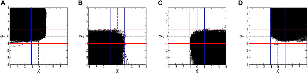
FIGURE 13. : Trajectories of tetraselmis in hyperbolic flow with A = 1.8 s−1. (These data exclude trajectories with classic run-and-tumble events during a trajectory.) The blue and red lines show the inward- and outward-blocking SwIM edges, respectively. (A) All trajectories that enter from the top and leave to the left. (B) All trajectories that enter from the bottom and leave to the left. (C) All trajectories that enter from the bottom and leave to the right. (D) All trajectories that enter from the top and leave to the right.
There are two main reasons for the differences between the behavior of the euglena and tetraselmis. First, since tetraselmis are more circular than euglena, there is less of a tendency for them to orient horizontally in the hyperbolic flow. Unlike with the euglena, the orientations are not readily visible in the microscopic images. We determine the orientations of the tetraselmis using the same technique used with the euglena, subtracting the flow velocity from the total trajectory velocities. The
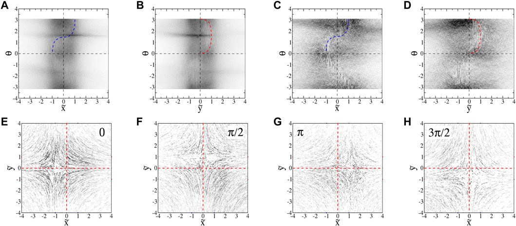
FIGURE 14. : Projections of
With swimming velocities that have non-zero
The swimming of the tetraselmis is also noisier than that of the euglena, even in the absence of classic run-and-tumble events. This can be seen qualitatively in the no-flow streak plots (Figure 4). The noisier motion results in a distribution of orientations (Figure 11B) that is much broader than that for euglena (Figure 11A). Furthermore, the distribution is significantly more broad for weaker flows, as seen by comparing the blue and red symbols in Figure 11B, qualitatively consistent with the theoretical predictions about the effects of noise on the angle distributions. Noise in the swimming orientations is another mechanism that causes non-zero y-components in the swimming that enable tracers to pass the passive manifold at
Plots of escape probability
5 Discussion
Overall, the experimental results are mostly consistent with predictions [33, 34] of swimming invariant manifolds as one-way barriers that impede the motion of self-propelled tracers in a hyperbolic fluid flow. In fact, the theory is quite robust. The swimming of both euglena and tetraselmis is not perfectly smooth and not even necessarily constant in time. Furthermore, the euglena are not even rigid—their shapes can undulate. Nevertheless, the SwIM theory still effectively predicts the one-way barriers that limit the motion of these microbes.
An important question is how to extend and apply SwIM theory to more realistic swimmers and more realistic flows. On the first point, it may be possible to modify the theory to account for swimming with a varying swimming speed, either by using perturbation methods for small variations in swimming speed or by explicitly adding terms to the
It would also be of interest to do experiments with self-propelled particles with negative α. Swimmers like this do not typically exist in nature, although it should be possible to fabricate synthetic swimmers such as Janus particles [31] that swim in a direction perpendicular to their semi-major axis. Of particular interest is the case where α = −1 where the system of equations Eq. 2a, Eq. 2b, Eq. 2c are the same as those for front propagation.
We are also interested in the importance of SwIMs on the simultaneous mixing of both passive and active tracers in the same flow [40], and the effects of chemotaxis on the nature of SwIMs as barriers for active mixing, especially in cases where a flow is mixing both the self-propelled tracers and also the nutrients toward which they exhibit chemotaxis. The effects of scattering of swimmers off physical boundaries [41] on the SwIMs is another important issue. Another problem of interest is the case where the behavior of the active tracers does alter the flow field (e.g., bacterial turbulence [42–44]), resulting in a self-consistent process whereby the swimmers generate a flow which then imposes barriers due to swimming invariant manifolds.
Data Availability Statement
The raw data supporting the conclusion of this article will be made available by the authors, without undue reservation.
Author Contributions
HY, JB, MD, and PJ developed the techniques that were used in collecting the data in these experiments. SB and KM provided frequent feedback on the analysis and comparison with theory; they also provided data for theoretical curves. TS ran the experiments, did most of the analysis and wrote the first draft of the manuscript. All authors contributed to the revision of the manuscript.
Funding
These experiments were supported by the National Science Foundation under grants DMR-1806355 and CMMI-1825379.
Conflict of Interest
Author PJ is employed by Velico Medical inc.
The remaining authors declare that the research was conducted in the absence of any commercial or financial relationships that could be construed as a potential conflict of interest.
Publisher’s Note
All claims expressed in this article are solely those of the authors and do not necessarily represent those of their affiliated organizations, or those of the publisher, the editors and the reviewers. Any product that may be evaluated in this article, or claim that may be made by its manufacturer, is not guaranteed or endorsed by the publisher.
Acknowledgments
The authors would like to thank Jack Raup for frequent assistance with the PDMS cells, Matthew Heintzelman for guidance on working with swimming microbes, and Brandon Vogel for initial assistance in working with PDMS.
Supplementary Material
The Supplementary Material for this article can be found online at: https://www.frontiersin.org/articles/10.3389/fphy.2022.861616/full#supplementary-material
Supplementary Video S1 | Movie corresponding to Figure 4B; motion of euglena without an imposed flow, shown with streaks.
Supplementary Video S2 | Movie corresponding to Figure 4B; motion of euglena without an imposed flow.
Supplementary Video S3 | Movie corresponding to Figure 4E; motion of tetraselmis without an imposed flow.
Supplementary Video S4 | Movie corresponding to Figure 4E; motion of tetraselmis without an imposed flow, shown with streaks.
Supplementary Video S5 | Movie corresponding to Figure 7A; motion of euglena with an imposed hyperbolic flow.
Supplementary Video S6 | Movie corresponding to Figure 7A; motion of euglena with an imposed hyperbolic flow, shown with streaks.
Supplementary Video S7 | Movie corresponding to Figure 12A; motion of tetraselmis with an imposed hyperbolic flow.
Supplementary Video S8 | Movie corresponding to Figure 12A; motion of tetraselmis with an imposed hyperbolic flow, shown with streaks.
References
1. Aref H. Stirring by Chaotic Advection. J Fluid Mech (1984) 143:1–21. doi:10.1017/s0022112084001233
2. Ottino JM. The Kinematics of Mixing: Stretching, Chaos and Transport. Cambridge: Cambridge University Press (1989).
3. MacKay RS, Meiss JD, Percival IC. Transport in Hamiltonian Systems. Physica D: Nonlinear Phenomena (1984) 13:55–81. doi:10.1016/0167-2789(84)90270-7
4. Rom-Kedar V, Wiggins S. Transport in Two-Dimensional Maps. Arch Rational Mech Anal (1990) 109:239–98. doi:10.1007/bf00375090
6. Camassa R, Wiggins S. Chaotic Advection in a Rayleigh-Bénard Flow. Phys Rev A (1991) 43:774–97. doi:10.1103/physreva.43.774
7. Solomon TH, Gollub JP. Chaotic Particle Transport in Time-dependent Rayleigh-Bénard Convection. Phys Rev A (1988) 38:6280–6. doi:10.1103/physreva.38.6280
8. Solomon TH, Tomas S, Warner JL. Role of Lobes in Chaotic Mixing of Miscible and Immiscible Impurities. Phys Rev Lett (1996) 77:2682–5. doi:10.1103/physrevlett.77.2682
9. Haller G. Lagrangian Structures and the Rate of Strain in a Partition of Two-Dimensional Turbulence. Phys Fluids (2001) 13:3365–85. doi:10.1063/1.1403336
10. Voth GA, Haller G, Gollub JP. Experimental Measurements of Stretching fields in Fluid Mixing. Phys Rev Lett (2002) 88:254501. doi:10.1103/physrevlett.88.254501
11. Mathur M, Haller G, Peacock T, Ruppert-Felsot JE, Swinney HL. Uncovering the Lagrangian Skeleton of Turbulence. Phys Rev Lett (2007) 98:144502. doi:10.1103/physrevlett.98.144502
12. Mezić I, Loire S, Fonoberov VA, Hogan P. A New Mixing Diagnostic and Gulf Oil Spill Movement. Science (2010) 330:486–9. doi:10.1126/science.1194607
13. Budisic M, Mezic I. Geometry of the Ergodic Quotient Reveals Coherent Structures in Flows. Physica D (2012) 241:1255
14. Haller G. Lagrangian Coherent Structures. Annu Rev Fluid Mech (2015) 47:137–62. doi:10.1146/annurev-fluid-010313-141322
15. Coulliette C, Lekien F, Paduan JD, Haller G, Marsden JE. Optimal Pollution Mitigation in Monterey bay Based on Coastal Radar Data and Nonlinear Dynamics. Environ Sci Technol (2007) 41:6562–72. doi:10.1021/es0630691
16. Di Giannatale G, Bonfiglio D, Cappello S, Chacón L, Veranda M. Prediction of Temperature Barriers in Weakly Collisional Plasmas by a Lagrangian Coherent Structures Computational Tool. Nucl Fusion (2021) 61:076013. doi:10.1088/1741-4326/abfcdf
17. Darwish A, Norouzi S, Labbio GD, Kadem L. Extracting Lagrangian Coherent Structures in Cardiovascular Flows Using Lagrangian Descriptors. Phys Fluids (2021) 33:11707. doi:10.1063/5.0064023
18. Serra M, Streichan S, Chuai M, Weijer CJ, Mahadevan L. Dynamic Morphoskeletons in Development. Proc Natl Acad Sci U.S.A (2020) 117:11444–9. doi:10.1073/pnas.1908803117
19. Mahoney J, Bargteil D, Kingsbury M, Mitchell K, Solomon T. Invariant Barriers to Reactive Front Propagation in Fluid Flows. Epl (2012) 98:44005. doi:10.1209/0295-5075/98/44005
20. Mahoney JR, Mitchell KA. Finite-time Barriers to Front Propagation in Two-Dimensional Fluid Flows. Chaos (2015) 25:087404. doi:10.1063/1.4922026
21. Bargteil D, Solomon T. Barriers to Front Propagation in Ordered and Disordered Vortex Flows. Chaos (2012) 22:037103. doi:10.1063/1.4746764
22. Megson PW, Najarian ML, Lilienthal KE, Solomon TH. Pinning of Reaction Fronts by Burning Invariant Manifolds in Extended Flows. Phys Fluids (2015) 27:023601. doi:10.1063/1.4913380
23. Gowen S, Solomon T. Experimental Studies of Coherent Structures in an Advection-Reaction-Diffusion System. Chaos (2015) 25:087403. doi:10.1063/1.4918594
24. Doan M, Simons JJ, Lilienthal K, Solomon T, Mitchell KA. Barriers to Front Propagation in Laminar, Three-Dimensional Fluid Flows. Phys Rev E (2018) 97:033111. doi:10.1103/PhysRevE.97.033111
25. Berg HC, Anderson RA. Bacteria Swim by Rotating Their Flagellar Filaments. Nature (1973) 245:380–2. doi:10.1038/245380a0
26. Stocker R, Durham WM. Tumbling for Stealth? Science (2009) 325:400–2. doi:10.1126/science.1177269
27. Rusconi R, Guasto JS, Stocker R. Bacterial Transport Suppressed by Fluid Shear. Nat Phys (2014) 10:212–7. doi:10.1038/nphys2883
28. Dehkharghani A, Waisbord N, Dunkel J, Guasto JS. Bacterial Scattering in Microfluidic crystal Flows Reveals Giant Active taylor-aris Dispersion. Proc Natl Acad Sci U.S.A (2019) 116:11119–24. doi:10.1073/pnas.1819613116
29. Brockmann D, Hufnagel L, Geisel T. The Scaling Laws of Human Travel. Nature (2006) 439:462–5. doi:10.1038/nature04292
30. Ebbens SJ, Howse JR. In Pursuit of Propulsion at the Nanoscale. Soft Matter (2010) 6:726. doi:10.1039/b918598d
31. Das S, Garg A, Campbell AI, Howse J, Sen A, Velegol D, et al. Boundaries Can Steer Active Janus Spheres. Nat Commun (2015) 6:8999. doi:10.1038/ncomms9999
32. Katuri J, Uspal WE, Simmchen J, Miguel-López A, Sánchez S. Cross-stream Migration of Active Particles. Sci Adv (2018) 4:eaao1755. doi:10.1126/sciadv.aao1755
33. Berman SA, Buggeln J, Brantley DA, Mitchell KA, Solomon TH. Transport Barriers to Self-Propelled Particles in Fluid Flows. Phys Rev Fluids (2021) 6:L012501. doi:10.1103/physrevfluids.6.l012501
34. Berman SA, Mitchell KA. Swimming Dynamics in Externally Driven Flows: The Role of Noise. Phys Rev Fluids (2022) 7:014501. doi:10.1103/PhysRevFluids.7.014501
35. Rom-Kedar V. Homoclinic Tangles-Classification and Applications. Nonlinearity (1994) 7:441–73. doi:10.1088/0951-7715/7/2/008
36. Torney C, Neufeld Z. Transport and Aggregation of Self-Propelled Particles in Fluid Flows. Phys Rev Lett (2007) 99:078101. doi:10.1103/PhysRevLett.99.078101
37. Khurana N, Blawzdziewicz J, Ouellette NT. Reduced Transport of Swimming Particles in Chaotic Flow Due to Hydrodynamic Trapping. Phys Rev Lett (2011) 106:198104. doi:10.1103/physrevlett.106.198104
38. Zöttl A, Stark H. Nonlinear Dynamics of a Microswimmer in Poiseuille Flow. Phys Rev Lett (2012) 108:218104. doi:10.1103/physrevlett.108.218104
39. Crocker JC, Weeks ER. Particle Tracking Using IDL (2011). Available at: http://physics.emory.edu/faculty/weeks/idl/.
40. Ran R, Brosseau Q, Blackwell BC, Qin B, Winter RL, Arratia PE. Bacteria Hinder Large-Scale Transport and Enhance Small-Scale Mixing in Time-Periodic Flows. Proc Natl Acad Sci U S A (2021) 118:e2108548118. doi:10.1073/pnas.2108548118
41. Chen H, Thiffeault J-L. Shape Matters: a Brownian Microswimmer in a Channel. J Fluid Mech (2021) 916:A15. doi:10.1017/jfm.2021.144
42. Dombrowski C, Cisneros L, Chatkaew S, Goldstein RE, Kessler JO. Self-concentration and Large-Scale Coherence in Bacterial Dynamics. Phys Rev Lett (2004) 93:098103. doi:10.1103/PhysRevLett.93.098103
43. Sokolov A, Aranson IS, Kessler JO, Goldstein RE. Concentration Dependence of the Collective Dynamics of Swimming Bacteria. Phys Rev Lett (2007) 98:158102. doi:10.1103/physrevlett.98.158102
Keywords: manifolds, active matter, dynamical systems, mixing, fluid dynamics, microfluidics
Citation: Yoest H, Buggeln J, Doan M, Johnson P, Berman SA, Mitchell KA and Solomon TH (2022) Barriers Impeding Active Mixing of Swimming Microbes in a Hyperbolic Flow. Front. Phys. 10:861616. doi: 10.3389/fphy.2022.861616
Received: 24 January 2022; Accepted: 22 March 2022;
Published: 25 April 2022.
Edited by:
Arlette R. C. Baljon, San Diego State University, United StatesReviewed by:
Eric Climent, UMR5502 Institut de Mecanique des Fluides de Toulouse (IMFT), FranceSanjeeva Balasuriya, University of Adelaide, Australia
Copyright © 2022 Yoest , Buggeln , Doan , Johnson , Berman, Mitchell and Solomon . This is an open-access article distributed under the terms of the Creative Commons Attribution License (CC BY). The use, distribution or reproduction in other forums is permitted, provided the original author(s) and the copyright owner(s) are credited and that the original publication in this journal is cited, in accordance with accepted academic practice. No use, distribution or reproduction is permitted which does not comply with these terms.
*Correspondence: Thomas H. Solomon , dHNvbG9tb25AYnVja25lbGwuZWR1
†Present Address: Helena Yoest, Applied Physics Laboratory, Johns Hopkins University, Laurel, MD, United StatesJohn Buggeln, Department of Physical Therapy, University of Delaware, Newark, DelawareMinh Doan, FPT University, Hanoi, VietnamPayton Johnson, Velico Medical, Beverly, MA, United States