Spectral Ultrasound Imaging of Speed-of-Sound and Attenuation Using an Acoustic Mirror

Speed-of-sound and attenuation of ultrasound waves vary in the tissues. There exist methods in the literature that allow for spatially reconstructing the distribution of group speed-of-sound (SoS) and frequency-dependent ultrasound attenuation (UA) using reflections from an acoustic mirror positioned at a known distance from the transducer. These methods utilize a conventional ultrasound transducer operating in pulse-echo mode and a calibration protocol with measurements in water. In this study, we introduce a novel method for reconstructing local SoS and UA maps as a function of acoustic frequency through Fourier-domain analysis and by fitting linear and power-law dependency models in closed form. Frequency-dependent SoS and UA together characterize the tissue comprehensively in spectral domain within the utilized transducer bandwidth. In simulations, our proposed methods are shown to yield low reconstruction error: 0.01 dB/cm⋅MHz^y for attenuation coefficient and 0.05 for the frequency exponent. For tissue-mimicking phantoms and ex-vivo bovine muscle samples, a high reconstruction contrast was achieved. Attenuation exponents in a gelatin-cellulose mixture and an ex-vivo bovine muscle sample were found to be, respectively, 1.3 and 0.6 on average. Linear dispersion of SoS in a gelatin-cellulose mixture and an ex-vivo bovine muscle sample were found to be, respectively, 1.3 and 4.0 m/s⋅MHz on average. These findings were reproducible when the inclusion and substrate materials were exchanged. Bulk loss modulus in the bovine muscle sample was computed to be approximately 4 times the bulk loss modulus in the gelatin-cellulose mixture. Such frequency-dependent characteristics of SoS and UA, and bulk loss modulus may therefore differentiate tissues as potential diagnostic biomarkers.

1 Introduction

Medical imaging methods aim to characterize and spatially map different soft tissue properties in order to provide diagnostic information regarding pathological structures and processes. Ultrasound imaging is a cost-effective, real-time and non-ionizing medical imaging modality. Conventional B-mode ultrasound imaging aims to map the amplitude of ultrasound waves scattered and reflected from tissue structures. Complementary to this, several methods exist in the literature to quantify various tissue characteristics. For instance, shear-wave elastography imaging (SWEI) aims to infer local soft tissue shear moduli, often derived from the group speed of propagating shear-waves that are induced using acoustic radiation force pushes [1,2]. Since soft tissues are inherently viscoelastic [3], several ultrasound-based imaging techniques were proposed to fully characterize the soft tissues in spectral domain by imaging the shear-wave speed [4–6] and shear-wave attenuation as a function of frequency [7–9], which then help to determine the shear and storage moduli of the medium. Methods also exist in the shear-wave literature that aim to characterize the nonlinear response of soft tissues given elastic [10–14] or viscoelastic [15–17] constitutive models and assumptions.

Inspired by such comprehensive mechanical characterization of soft tissue using group speed, phase velocity, and attenuation of shear waves as a function of frequency, we herein propose to extend similar characterization to ultrasound waves themselves. Ultrasound is a longitudinal (compressional) mechanical wave, and through its propagation in tissues, its characteristics also change based on tissue mechanical properties. Accordingly, ultrasonic group speed, phase velocity, and attenuation as a function of frequency can be used for further characterization of soft tissues. Indeed, ultrasound group speed (commonly called speed-of-sound, SoS) is related to medium bulk modulus while phase velocity and attenuation are related to bulk storage and loss moduli. Imaging of (group) SoS has been studied in the literature using tomographic approaches with custom made ultrasound transducer and data acquisition solutions in [18–20], which involve bulky and costly setups and submersion of the imaged anatomy in water. To utilize the practical advantages of commercial transducer arrays, SoS imaging using conventional transducers in pulse-echo mode has been proposed recently, following two approaches: A group of methods measure apparent displacements of backscattered signals when insonified from different angles [21–23]. Alternative methods use an additional passive acoustic reflector on the opposite side of the imaged anatomy to measure several time-of-flight values from which to tomographically reconstruct local SoS distribution [24,25].

Similarly to SoS imaging, imaging ultrasound attenuation (UA) was also proposed using custom-made water-submersion setups [18]. Using conventional ultrasound transducers, some methods utilize the fact that the ultrasound center frequency decreases as a function of propagation depth and medium UA, since attenuation affects higher frequencies more prominently. Based on this, a spectral difference method [26] and spectral log difference methods [27,28] were proposed using typical B-mode images together with reference phantom measurements. An adjacent frequency normalization was proposed in [29] to cancel out systemic effects such as focusing and time-gain-compensation without the need of reference phantom measurements. Alternatively, reference measurements from a passive acoustic mirror was used in [30,31] to estimate UA values, however this requires apriori segmentation masks to be given and hence do not allow the UA imaging of arbitrary unknown domains. Recently, imaging of local UA has been proposed in [32] using a limited-angle computed tomography (LA-CT) method.

Formally, UA α(ω) is a function of ultrasound frequency ω and it typically follows a power-law relation of the form α(ω) = α₀ω^y, where α₀ is called the attenuation coefficient and y the power exponent. The above-mentioned methods in the literature either estimate a single UA map, e.g., at the ultrasound transmit center frequency or estimate the attenuation coefficient α₀ map assuming y = 1. The latter assumption of y ≈ 1 is not necessarily valid in general as it was shown that soft tissues exhibit varying UA power exponents y [26,33]. Furthermore, using a single (center) frequency for the analysis neglects the fact that the spectral composition of propagating waves change given the larger attenuation at higher frequencies. Characterizing UA using a parametric model over a frequency range would enable a complete spectral characterization. This would allow for treating the UA variation within the utilized bandwidth as information, which is treated as noise when the underlying model is neglected. The parameters of such model can also yield additional imaging biomarkers characterizing the spectral tissue behaviour. With this motivation, recently in [34] it was proposed to reconstruct multiple UA maps (α) at different band-pass filtered frequency bands. To estimate α₀ and y locally, these UA maps were then pixel-wise fitted with a power-law model by assuming the UA estimates to characterize the response at the central frequency of each band. However, band-pass filtering the signal over a frequency band then averages the cumulative effect of the entire frequency band. Also, the pixel-wise model fitting ignores the spatial continuity of the image, where the individual frequency band reconstructions cannot benefit from each other and the SNR loss due to dividing into separate pass-bands cannot be recovered. A frequency-domain solution, similar to those in shear-wave applications and which takes into account the entire bandwidth in a single inverse problem formulation, could mitigate the above shortcomings and is proposed herein for UA reconstruction.

Similarly to UA, SoS also varies not only across tissues, e.g., in the human liver depending upon water, fat, and collagen concentrations [33], but also across acoustic frequencies [35–38]. SoS is shown to vary with respect to frequency in soft tissues in the literature [39]. For instance, it was shown in [40] that SoS varies with frequency in human brain tissues. Thus, frequency-dependent characterization of SoS may be an additional biomarker for tissue characterization.

In this study, we introduce a new method based on general wave theory in frequency domain to compute both SoS and UA across frequencies and compute the SoS and UA model parameters together using a inverse problem formulation. We have conducted simulations and ex-vivo phantom studies to discuss the reconstruction results.

2 Methods

We acquire ultrasound data in multistatic mode, in which a single transducer element at a time is used for transmitting (Tx) a broadband ultrasound pulse into the medium and an acoustic mirror is placed at a predefined distance from the ultrasound transducer surface. The reflected ultrasound echoes are recorded as received (Rx) with all the transducer elements. This process is repeated until all the transducer elements are used for the transmission. Multistatic data acquisition is schematically described in Figure 1A for transmission with an element and receiving at different transducer elements with varying path lengths (marked with different colors). Full-matrix multistatic data is then processed using the algorithm in [41] to delineate the reflector profile in the echoes reflected from the acoustic reflector positioned at a pre-defined depth. A sample delineation for Tx#64 of a 128 element transducer is marked on the pre-beamformed channel data in Figure 1B. Other high amplitude echo profiles below the first arrival echoes seen in Figure 1B correspond to reflections from different interfaces of the acoustic reflector, for more details please refer to Figure 1 in [41]. Sample cropped reflector echo profiles for Tx#64 and Rx#{8,16, … ,120} are plotted in Figure 1C. For reconstruction of SoS and UA at a particular frequency we use phase spectrum and amplitude spectrum values, respectively, obtained by the Fourier transform (FT) of the above echo profiles around the delineated reflector time points. Phase and amplitude spectrums for some of the echo profiles shown in Figure 1 are plotted in Figures 2A,B respectively. For reconstruction of SoS and UA at a particular frequency we use the amplitude and phase spectrum values at that frequency, for all combinations of Tx-Rx as shown in Figures 2C,D. These phase and amplitude spectrum readings for all Tx-Rx combinations are then corrected using pre-acquired calibration measurements in water, cf. Figures 2E,F, which are used for solving inverse problems to reconstruct SoS and UA at that chosen frequency as shown in Figures 2G,H. The above method overview is elaborated and detailed in the following sections.

FIGURE 1

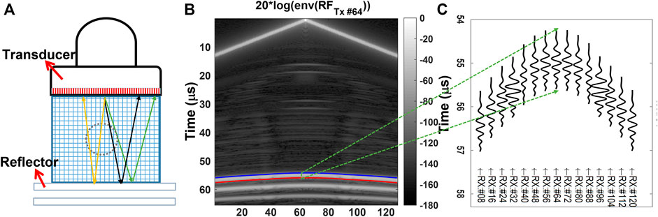
FIGURE 1. (A) Schematic of the imaging setup where an acoustic mirror (reflector) is positioned at a pre-defined distance from the ultrasound transducer surface, with coloured paths representing the traversal of different acoustic wavefront paths from a single transmit element to different receivers through a discretized tissue representation, (B) Pre-beamformed data received by all the receive channels of the transducer when the transducer element #64 is used for transmission (Tx). (C) Cropped reflector echo profiles corresponding to different Rx elements, from which the reflector is next delineated precisely.

FIGURE 2

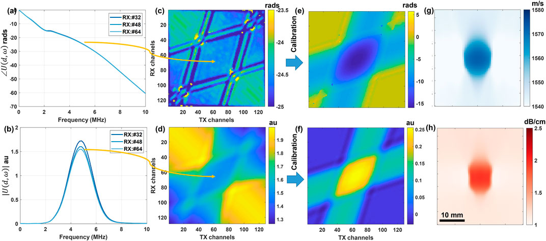
FIGURE 2. Procedure of estimating SoS and UA distribution maps at frequency ω. 1D temporal Fourier transform is performed on the echo profiles obtained at different Rx channels to obtain (A) phase spectrum ∠U (d, ω) and (B) amplitude spectrum |U (d, ω)| for three sample profiles shown in Figure 1C. Phase and amplitude spectrum values for all Tx-Rx combinations at a selected sample frequency of 5 MHz are shown, respectively, in (C) and (D). These values are then calibrated as described in Sec. 2.2 leading to the calibrated phase (E) and amplitude (F) spectrum values, which are used for solving inverse problems to reconstruct local SoS (G) and UA (H) distributions at ω.

2.1 Ultrasound Wave Propagation in Viscoelastic Medium

As a broadband ultrasound wave passes through a medium, its waveform changes according to the phase velocity and attenuation of the medium. Ultrasound waves travelling through a viscoelastic medium can be defined in the frequency domain as:

$U\left(d,\omega \right)=G\left(\omega \right)e^{-i\widehat{k}\left(\omega \right)d}(\mathrm{1a})$

$\mathrm{w}\mathrm{i}\mathrm{t}\mathrm{h}\widehat{k}\left(\omega \right)=\frac{\omega }{c\left(\omega \right)}-i\alpha \left(\omega \right)(\mathrm{1b})$

where U (d, ω) is the FT of the ultrasonic wave u (d, t), ω is the angular frequency, d is the propagation distance, $\widehat{k}(\omega )$ is the complex wave number, c(ω) is the phase velocity, and α(ω) is attenuation at ω, and G(ω) accounts for the transmit and receive transducer responses at frequency ω.

As seen in Eq. 1a, ultrasonic wave amplitude decreases as a function of propagation distance d due to absorption, relaxation, scattering, etc. Indeed using this wave equation, ultrasound phase velocity and attenuation can be derived using amplitude and phase spectrums by taking the natural logarithm of amplitude |U (d, ω)| and separating the phase terms to equate to phase angle ∠U (d, ω), which yield respectively:

$\angle U\left(d,\omega \right)=\frac{\omega }{c\left(\omega \right)}d+\angle G\left(\omega \right),(\mathrm{2a})$

$\ln \left(|U\left(d,\omega \right)|\right)=\ln \left(G\left(\omega \right)\right)-\alpha \left(\omega \right)d.(\mathrm{2b})$

2.2 Forward Problem of Ultrasound Wave Propagation

Phase and amplitude spectra for the reflector echo corresponding to Tx element t and Rx element r relates, respectively, to slowness s_p(ω) = 1/c(ω), i.e., the inverse of phase velocity, and attenuation α(ω) along the traversed ray path p as follows:

$\angle U_{t,r}\left(\omega \right)=\omega {\int }_{p}s\left(\omega \right)\mathrm{d}l+\angle G_{t,r}\left(\omega ,{\theta }_{t,r}\right),(\mathrm{3a})$

$|U_{t,r}\left(\omega \right)|=\exp \left(-{\int }_p\alpha \left(\omega \right)\mathrm{d}l\right)+|G_{t,r}\left(\omega ,{\theta }_{t,r}\right)|.(\mathrm{3b})$

where p represents the acoustic ray path and l is the traversed distance. ∠G_t,r (ω, θ_t,r) and |G_t,r (ω, θ_t,r)| are the confounding factors attributable to transducer Tx-Rx phase and amplitude transfer characteristics at different angles (e.g., the aperture opening and side-lobes) as well as the acoustic reflector reflection characteristics, i.e., the incidence angle dependent specular and diffuse reflection and transmission characteristics of the reflector surface. These have to be compensated for in order to be able to measure the actual ultrasound phase velocity and attenuation effects. For this purpose, we calibrate these measurements by normalizing with measurements in water $(U_{t,r}^{water}(\omega ))$ at a known water temperature and using the same ultrasound pulses (bandwidth) as in the targeted tissue imaging setup. From the given water temperature, we compute the ground-truth water SoS using the relationship in [42], which was 1,483.1 m/s in our setup. Water UA is known from [43] to be α(f) = 2.17 × 10⁻¹⁵f².

We used the procedure described in [34] to compensate for the confounding effects in |G_t,r (ω, θ_t,r)|. The reflector does not change the phase of the reflected ultrasound signals, since its acoustic impedance is higher than water and soft tissues. Thus, for factoring out the confounding effects in ∠G_t,r(ω), we used simply the phase angles of reflector echo profiles from water calibration experiments. We denote these calibrated amplitude and phase spectrum values as $|U_{t,r}^{\prime }(\omega )|$ and $\angle U_{t,r}^{\prime }(\omega )$, respectively, which are given by

$\angle U_{t,r}^{\prime }\left(\omega \right)=\angle U_{t,r}\left(\omega \right)-\angle U_{t,r}^{\text{water}}\left(\omega \right)(\mathrm{4a})$

$|U_{t,r}^{\prime }\left(\omega \right)|=\frac{U_{t,r}\left(\omega \right)R_{\text{water}}\left(\theta \right)}{U_{t,r}^{\text{water}}\left(\omega \right)R\left(\theta \right)}.(\mathrm{4b})$

where R_water(θ) and R(θ) are the ultrasound reflection coefficients of the reflector in water and in targeted imaging medium, respectively, for incident angle θ. It can be estimated using Snell’s law with the SoS in water (c_water) and an approximate SoS of the targeted medium, as in [34].

For acoustic propagation, refractions are herein ignored and the travel of acoustic wave from a transmitting to receiving element is modeled using a straight ray approximation as depicted in Figure 1A. For a straight acoustic path, the first wavefront from a Tx element, reflecting from the reflector and arriving at an Rx element can be assumed to follow the shortest path, thus being reflected at the mid-point between these Tx and Rx element locations projected on the reflector, cf. Figure 1A. To cast this as a tomographic reconstruction problem, the relation in Eq. 3 above can be discretized on a Cartesian grid as

$\angle U_{t,r}^{\prime }\left(\omega \right)=\omega \sum _{n=1}^{N_i}{s}_k\left(\omega \right)l_{ik},(\mathrm{5a})$

$|U_{t,r}^{\prime }\left(\omega \right)|=\exp \left(-\sum _{n=1}^{N_i}{\alpha }_k\left(\omega \right)\mathrm{d}l\right).(\mathrm{5b})$

where s_k(ω) and α_k(ω) represents the slowness and attenuation, respectively, in pixel k along ray i spanning N_i pixels, where l_ik represents the partial acoustic path length of ray i within this pixel k.

Collocating Eq. 5 for each ray path along all Tx-Rx combinations and taking logarithm on both sides of Eq. 5b, the forward-problem of ultrasound propagation can then be represented with the following systems of linear equations

$\omega \mathbf{L}\mathrm{s}\left(\omega \right)=\varphi \left(\omega \right),(\mathrm{6a})$

$\mathbf{L}\alpha \left(\omega \right)=b\left(\omega \right),(\mathrm{6b})$

where ϕ(ω) and b(ω) are, respectively, the column vectors of phase $\angle U_{t,r}^{\prime }(\omega )$ and amplitude $\ln |U_{t,r}^{\prime }(r,\omega )|$ values along all ray paths at frequency ω; s(ω) and α(ω) are the column vectors of, respectively, the slowness and attenuation values for all reconstruction grid pixels at frequency ω; and the system matrix L encodes the discretized ray integrals for each ray onto the pixel grid as in [25]. Note that L is constant for given transducer geometry and reflector position.

2.3 Reconstruction of Phase Velocity and Attenuation

Given calibrated phase spectrum ϕ(ω) and amplitude spectrum b(ω) measurements, one can then reconstruct the local slowness and UA maps at frequency ω by solving the following inverse problems:

$\widehat{s}\left(\omega \right)=\arg \underset{s\left(\omega \right)}{\min }\Vert \omega \mathbf{L}\mathrm{s}\left(\omega \right)-\varphi \left(\omega \right){\Vert }_1+\lambda \Vert Ds\left(\omega \right){\Vert }_1(\mathrm{7a})$

$\widehat{\alpha }\left(\omega \right)=\arg \underset{\alpha \left(\omega \right)}{\min }\Vert \mathbf{L}\alpha \left(\omega \right)-\mathrm{b}\left(\omega \right){\Vert }_1+\lambda \Vert D\alpha \left(\omega \right){\Vert }_1(\mathrm{7b})$

where λ is the weight parameter of regularization required to help robustly solve these ill-posed problems. Similarly to [22,25,32,34], we herein use l₁-norm for both the data and regularization terms for robustness to outliers in, respectively, the measurements and the reconstructions [44]. For regularization, in order to suppress the typical streaking artifacts associated with LA-CT due to missing orthogonal projections as well as the uneven distribution of measurement paths, we use anisotropic weighting of directional gradients proposed in [45], with a weighting of k = 0.9 as in [25]. Accordingly, the regularization matrix D is composed of a mix of Sobel (axis-aligned) and Robert (diagonal) kernels with corresponding weights and locations, as in [23]. In this paper we empirically set λ = 0.6 for all experiments of phase velocity and UA reconstructions. For the numerical solution of the optimization problem Eq. 7, a limited-memory Broyden-Fletcher-Goldfarb-Shanno (L-BFGS) algorithm [46–49] is used from the unconstrained optimization package minFunc¹.

2.4 Model Fitting

Ultrasound phase velocity c(ω) and attenuation α(ω) reconstructions are computed for a range of frequencies [ω_c − nΔω, … , ω_c, … , ω_c + nΔω] around the center frequency ω_c of the ultrasound pulse with Δω being the frequency resolution used for computing the FT of the reflector profiles. Sample reconstructions at three frequency values are shown in Figures 3A,B. Phase velocities for wide range of frequencies may exhibit complex profiles as in [50–52]. Nevertheless, for small ranges of ultrasound imaging frequencies, such frequency dependence can be approximated with a linear disperse model, similarly to the shear-wave phase velocity studies in [16,53]. Given the relatively small bandwidth of the utilized ultrasound pulse, the phase velocity is expected to vary linearly within this bandwidth, as illustrated by two sample profiles in Figure 3C. For frequency characterization of attenuation, it is well known in the literature that attenuation as a function of frequency obeys the power-law, which corroborates the observation in Figure 3D. One could fit these models pixel-wise for the given range frequencies and solve for the model parameters in the least square sense, as in [34]. However, this may be error prone as it ignores the spatio-spectral continuity in the medium. Herein, we incorporate frequency-dependent models of speed and attenuation into the reconstruction process, such that the inverse problem solution is informed by and can leverage the measurements at each frequency and path concurrently, while estimating the frequency-dependent medium parameters.

FIGURE 3

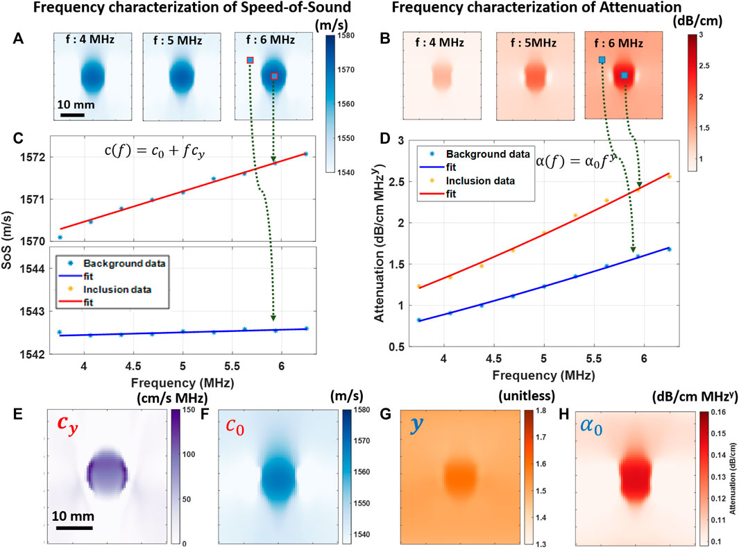
FIGURE 3. Illustration of parameter estimation for SoS and UA on a sample simulated numerical phantom: SoS (A) and UA (B) reconstructions at frequencies f = {4, 5, 6} MHz obtained by following the procedure in Figure 2. Fitting frequency-dependent models as in Eqs. 8 for SoS (C) UA (D) at two sample locations inside and outside the inclusion. By solving the inverse problem in Eq. 9, spatial distributions of the following model parameters are obtained: SoS coefficient i.e., c_y (E), SoS dispersion coefficient c₀ (F), UA power-law exponent y (G), and UA coefficient α₀ (H).

As models of the frequency-dependent nature of ultrasound phase velocity and attenuation, we use herein the following linear and power-law relations, respectively:

$c\left(f\right)=c_0+c_{y}f(\mathrm{8a})$

$\alpha \left(f\right)={\alpha }_0{f}^y;(\mathrm{8b})$

where c(f) and α(f) are the frequency-dependent SoS and attenuation, c₀ and α₀ the medium-specific SoS and attenuation coefficients, c_y the medium-specific SoS dispersion coefficient, and y the medium-specific attenuation exponent.

By colocating SoS reconstructions for all measurement frequencies from Eq. 7a in Eq. 8a, a comprehensive system of equations that encodes both SoS model parameters for all image locations is arrived as follows:

$\widehat{\mathit{\theta }}=\arg \underset{\mathit{\theta }}{\min }\Vert A\mathit{\theta }-\mathit{v}{\Vert }_1+\lambda \Vert D^{\prime }\mathit{\theta }{\Vert }_1(9)$

where $\mathit{\theta }={\left[{\mathbf{c}}_0{\mathbf{c}}_{\mathbf{y}}\right]}^{\mathrm{T}}$, $\mathit{v}={\left[{\mathbf{c}}_{{\mathbf{f}}_1}{\mathbf{c}}_{{\mathbf{f}}_2}\cdots {\mathbf{c}}_{{\mathbf{f}}_{\mathbf{n}}}\right]}^{\mathrm{T}}$, D′ = [D D], and

$A=\left[\begin{array}{cc}\hfill I_{n_p}\hfill & \hfill f_1\ast I_{n_p}\hfill \\ \hfill I_{n_p}\hfill & \hfill f_2\ast I_{n_p}\hfill \\ \hfill ⋮\hfill & \hfill ⋮\hfill \\ \hfill I_{n_p}\hfill & \hfill f_n\ast I_{n_p}\hfill \end{array}\right]$

with bold variables denoting size-n_p row vectors of the sought parameters in the imaged field-of-view, $I_{n_p}$ is the identity matrix of size n_p and n_p is the total number of reconstruction grid pixels.

For estimating UA parameters, we colocate UA reconstructions for all measurement frequencies from Eq. 7b in Eq. 8b. Taking the logarithm of both sides (in order to drop down the exponent) a similar linear problem as in Eq. 9 is arrived, but this time with the variables $\mathit{\theta }={\left[\log {\mathit{\alpha }}_0,\mathit{y}\right]}^{\mathrm{T}}$, $\mathit{v}={\left[\log {\mathit{\alpha }}_{{\mathbf{f}}_1},\log {\mathit{\alpha }}_{{\mathbf{f}}_2},\dots ,\log {\mathit{\alpha }}_{{\mathbf{f}}_{\mathbf{n}}}\right]}^{\mathrm{T}}$, and

$A=\left[\begin{array}{cc}\hfill I_{n_p}\hfill & \hfill \log \left(f_1\right)\ast I_{n_p}\hfill \\ \hfill I_{n_p}\hfill & \hfill \log \left(f_2\right)\ast I_{n_p}\hfill \\ \hfill ⋮\hfill & \hfill ⋮\hfill \\ \hfill I_{n_p}\hfill & \hfill \log \left(f_n\right)\ast I_{n_p}\hfill \end{array}\right].$

Solving these inverse problem formulations we estimate the spatial maps of SoS model parameters c₀ and c_y, and of UA model parameters α₀ and y. Sample reconstructions from the earlier simulated example can be seen in Figures 3E–H.

2.5 Complex Bulk Modulus

Given ultrasound phase velocity c(ω) and attenuation α(ω) maps reconstructed above, complex bulk modulus $\widehat{K}$ can be determined in a model-independent way to characterize the viscoelastic nature of the tissue through its relationship to complex wave number as follows:

$\widehat{K}\left(\omega \right)=K^{\prime }\left(\omega \right)+i{K}^{″}\left(\omega \right)=\frac{\rho {\omega }^2}{{\widehat{k}}^2\left(\omega \right)},(10)$

where ρ represents tissue density. Substituting Eq. 1b in Eq. 10 allows to derive the bulk storage modulus K′ and bulk loss modulus K^″ as follows:

$K^{\prime }\left(\omega \right)=\rho {\omega }^2\frac{{\left(\frac{\omega }{c\left(\omega \right)}\right)}^2-\alpha {\left(\omega \right)}^2}{{\left({\left(\frac{\omega }{c\left(\omega \right)}\right)}^2+\alpha {\left(\omega \right)}^2\right)}^2},(\mathrm{11a})$

$K^{″}\left(\omega \right)=2\rho {\omega }^2\frac{\left(\frac{\omega }{c\left(\omega \right)}\right)\alpha \left(\omega \right)}{{\left({\left(\frac{\omega }{c\left(\omega \right)}\right)}^2+\alpha {\left(\omega \right)}^2\right)}^2}.(\mathrm{11b})$

2.6 Evaluation Metrics

In this study, the following metrics are used for a quantitative analysis of the simulation results:

• Root-mean-squared-error (RMSE)

     $RMSE=\sqrt{\frac{1}{n_p}{\left(x^{\star }-\widehat{x}\right)}^2}$, where x represents a reconstructed parameter map with the number of pixels n_p. The ⋅^⋆ and $\widehat{\cdot }$ indicate, respectively, the ground-truth and a reconstruction.

• Contrast-ratio fraction (CRF)

     $CRF=\frac{\widehat{C}}{C^{\star }}$, where $C=\frac{|{\mu }_{\text{inc}}-{\mu }_{\text{bg}}|}{|{\mu }_{\text{inc}}|+|{\mu }_{\text{bg}}|}$ with mean inclusion and background values μ_inc and μ_bg, respectively, where the inclusion is delineated using the ground-truth map.

• Contrast-to-noise ratio (CNR)

     $CNR=\frac{|{\mu }_{\text{inc}}|-|{\mu }_{\text{bg}}|}{\sqrt{{\sigma }_{\text{inc}}^2+{\sigma }_{\text{bg}}^2}}$, where σ² represents the variance.

2.7 Simulation Experiments

Numerical simulations were conducted to study the reconstruction accuracy of the proposed methods. These simulations were conducted by varying local distribution of SoS and UA patterns and varying their frequency dependency characteristics. An open-source acoustics toolbox k-Wave [54] was used for this purpose. k-Wave uses Kramers–Kronig relations [50–52] to simulate the dispersive phase speed based on given spatial maps of UA coefficient α₀ (x, y) and SoS $c_{f_c}(x,y)$ at the center frequency, as well as the power-law dependency parameter y. Note that in k-Wave, y is a single constant for the entire domain/simulation and cannot be controlled spatially.

The transducer was simulated as a linear array of 128 elements with a pitch of 0.3 mm. Full-matrix multistatic data was simulated at a center frequency of 5 MHz with a 5-cycle input pulse. For the simulation, we used a temporal resolution of 160 MHz and a spatial grid resolution of 37.5 μm. In the physical experimental setup, the acoustic mirror is made of plexiglass, so it was simulated using plexiglass’s acoustic properties (density ρ = 1180 kg/m³, SoS c = 2700 m/s), as positioned at a distance of 42 mm from the transducer surface in all three simulations. A single circular inclusion with 5 mm radius is placed at the center of the imaging field-of-view. SoS at center frequency $(c_{f_c})$ in the background and inclusion were set, respectively, 1,540 m/s and 1,601.6 m/s (for 4% contrast). The inclusion and background attenuation coefficient (α₀) were set, respectively, 0.2 dB/cm⋅MHz^y and 0.1 dB/cm⋅MHz^y.

We repeated the simulations three times by varying the power exponent y = {1.1, 1.5, 1.9}, which led to three numerical phantoms referred hereafter as sim{#1, #2, #3}, respectively. Note that given constraints in k-Wave, SoS and UA cannot be controlled independently and arbitrarily, and the variation of such exponent y changes both SoS and UA with a known relation.

2.8 Phantom and ex-Vivo Experiments

These were conducted using the data from [34]. In the first phantom #A we used, the background has 10% gelatin 1% Sigmacell Cellulose Type 50 (Sigma Aldrich, St. Louis, MO, United States), into which a bovine skeletal muscle sample was inserted as an inclusion. For the second phantom #B, the background and inclusion compositions were interchanged, i.e., a gelatin phantom piece was inserted as the inclusion inside a bulk muscle sample. Data acquisitions were conducted on a research ultrasound machine (Verasonics, Kirkland, WA, United States) with a 128-element linear-array transducer (Philips, ATL L7-4). Similarly to the simulation setup, a wideband Tx pulse with a center frequency of 5.2 MHz and a pulse length of five cycles was used. For the calibration procedure, multi-static data sets were acquired in distilled water at room temperature by placing the reflector at multiple depths {31, 35, 39, 43, 47} mm. For any intermediate reflector depths used in the phantom measurements, calibration data was interpolated from the available water measurements above, as described in [32].

3 Results and Discussion

First, the reflector profiles are delineated in the multistatic data for each Tx event using [41]. To identify the acoustic reflector surface, we tuned this reflector delineation framework to use the so-called “edge” feature with a window length of 200 and 50, respectively, for simulations and ex-vivo experiments. A cubic RANSAC [55] model was used for outlier removal, to estimate an initial contour, which was next refined using an optimization-based active contours [56] method, which hence utilizes the expected temporal continuity of the neighbouring profiles for a robust estimation. This then yields the final delineation of reflector echoes to estimate the time-of-flights as well as the temporal echo profiles around the delineated reflector surface (to further process) as exemplified in Figure 1C. This delineation procedure was repeated for all 128 Tx events. For each delineated reflector profile of a Tx-Rx combination, 43 RF samples (within which the surface echo is observed, also corresponding roughly to the 5 cycles of a Tx pulse) around the delineated location is taken out, zero-pad to 128 samples, and input to a 1-D temporal Fourier transform using FFT, leading to a spectral resolution of 312.5 and 325.5 kHz, respectively, for simulations and ex-vivo experiments. The above yields phase and amplitude spectrums, as exemplified in Figures 2A,B. Repeating this for all Tx-Rx combinations yields 128 × 128 spectrum profiles for phase and amplitude. Next, phase and amplitude values at a frequency of interest are extracted and calibrated using the respective calibration parameters, derived separately for (simulated) numerical and physical experiments. From the calibrated measurements for all Tx-Rx combinations, SoS and UA maps are reconstructed using Eqs 7–9).

System matrix L is constant for given transducer geometry and reflector position. It, however, needs to be recomputed if the reflector distance changes, e.g., based on the imaged organ’s physical dimension. Nevertheless, L can be precomputed for several potential imaging distances and loaded at imaging time based on the current reflector distance. It is further possible to have a reflector setup where physical distances are constrained mechanically to certain increments as in [45]. Reconstruction of SoS or UA at a single frequency takes ≈8.2 s. Assuming that this can be parallelized for multiple frequencies we utilize and by using L and D matrices precomputed for a given distance, then our proposed reconstruction including preprocessing for reflector delineation and postprocessing by parameter fitting would take 12.6 s, using unoptimized MATLAB code. Single frequency reconstructions or the overall parameter estimation can be accelerated to real-time via loop-unrolling of tomographic reconstruction using variational networks as in [57,58].

We assume that reconstructions are thin planar slices, although ultrasound propagation has a finite elevational thickness, e.g. attenuations caused by out-of-plane structures. Nevertheless, such out-of-plane effects are less likely to affect measurements with a reflector where only specular (direct) reflections arrive back at a receive element.

3.1 Simulation Results

SoS and UA reconstructions for sim#2 are presented in Figure 2. Reconstructed c₀ (i.e., SoS at the center frequency c (f_c)) and the linear dispersion coefficient c_y for the three simulations are depicted in Figure 4. From the ground-truth and reconstructed SoS maps at the center frequency in Figures 4A,B, it can be seen that the background SoS at the center frequency is reconstructed with some success in all cases. However, the inclusion SoS values are seen to be shifted towards background values, which corroborates the findings in [25]. This is due to the limited-angle tomographic nature of the problem, where the lack of lateral projections combined with the regularization needed for robust solutions cause the smoothing and axial elongation of the inclusions, hence spreading them over a larger area. Since the cumulative SoS effect shall stay the same, per-pixel inclusion values are effectively averaged with the background, inversely proportional to such artifactual area increase.

FIGURE 4

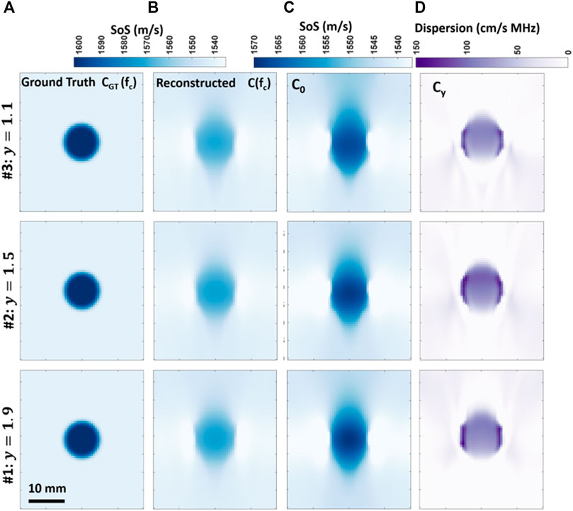
FIGURE 4. Comparison of frequency-dependent SoS imaging for the three different simulations with y = {1.1, 1.5, 1.9} in each row, with columns from left to right (A-D): ground-truth SoS maps c_GT (f_c) at the center frequency f_c = 5 MHz; reconstructed SoS maps c (f_c) at the center frequency; reconstructed c₀ maps; and reconstructed c_y maps.

Note that as y varies across the simulations, so does c_y, according to Kramers–Kronig relationship [51]. Therefore, the c_y maps in Figures 4D are expected to present contrast between the three simulations with different y values. An analytical computation of expected SoS dispersion in the utilized frequency range of 4–6 MHz according to the Kramers–Kronig relationship is illustrated in Figure 5. Accordingly, in this frequency range a linear SoS dispersion (c_y) of {6.5, 9.7, 5.3} cm/s⋅MHz for the background and {14.1, 21.0, 11.4} cm/s⋅MHz for the inclusion are expected for each respective simulation. These are used as ground-truth c_y values for the following evaluation.

FIGURE 5

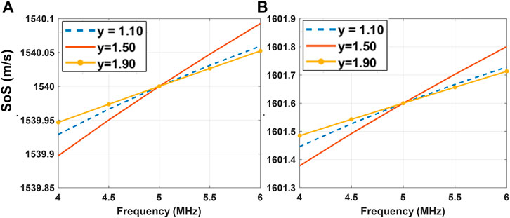
FIGURE 5. SoS dispersion characteristics for the background (A) and inclusion (B) for k-Wave simulations with power-law exponent y = {1.1, 1.5, 1.9} according to the Kramers–Kronig relationship that is being used in the simulation toolbox k-Wave [50–52].

For a quantitative evaluation, we computed the metrics RMSE, CNR, and CRF for each simulation, as reported in Table 1. We computed the mean and standard deviation for the background and inclusion using their respective masks from simulations. The average RMSE of c (f_c) is 8.50 ± 0.24 m/s and the average mean values of c (f_c) in the background region is 1,542.3 ± 0.1 m/s, demonstrating that an accurate reconstruction of the speed of sound is possible. The contrast metrics CNR and CRF for c (f_c) and for c₀ indicate that the inclusions can be successfully distinguished in SoS reconstructions, with a contrast similar to their prescribed ground-truth value. Note that c_y reconstructions for all the simulations show large RMSE errors of 39–53 cm/s⋅MHz. This is mainly due to the relatively minute dispersion values of [5.3–9.7] cm/s⋅MHz and hence their minimal effect in SoS change within the given frequency interval (see the changes in y-axis in Figure 5 being $<$0.4 m/s for inclusion $<$0.2 m/s for the background). Note that this is partly due to our earlier-mentioned experimental limitations with k-Wave parameterizations, where SoS frequency dispersion can only be generated by varying y, which then has a much more prominent impact on UA. To capture such variation, very high SNR and precision would be required in SoS reconstructions. Despite the accuracy being low for these, nevertheless, the relative differences and contrasts are recovered successfully: For instance, c_y for the inclusion of sim #2 is higher than that of sim #1 and #3, which corroborates the analytical expectation from Figure 5. Similarly, corroborating the analytical expectation, the inclusions in sim #1 and #2 show roughly twice the dispersion that their backgrounds. The average ratio of ${\mu }_{inc}^{c_y}$ to ${\mu }_{bg}^{c_y}$ is ≈2.4, which is close to the ground truth c_y contrast of 2 between inclusion and background. Therefore, despite not being accurate reconstructed c_y values are still correlated with ground truth counter-parts and hence may potentially act as an imaging biomarker.

TABLE 1

TABLE 1. Quantitative evaluation of SoS and UA frequency-dependent model parameter reconstructions for simulations. μ_bg and σ_bg are mean and standard deviation of background, μ_inc and σ_inc are mean and standard deviation of inclusion.

Reconstructed UA at the center frequency α_fc, UA coefficient α₀, and exponent y are plotted in Figure 6. Given the groundtruth and reconstructed α_fc maps in Figures 6A,B, it can be seen that the UA at center frequency is successfully reconstructed in all cases. In Figures 6B,C it is observed that the reconstructed α_fc and α₀ values in the inclusions are shifted towards the background values, similarly to SoS results in Figure 4B and also in line with previous observations in [34]. The UA exponent y maps in Figure 6C should not present any contrast since the power exponent y are constant across each domain. Although this is true for sim #1, the other two simulations exhibit a slight deviation of y in the inclusion region. This is due to the relatively more pronounced artifactual elongations of the inclusion in UA reconstructions with increased frequency dispersion, which then slightly reduce the per-pixel reconstructed UA value (through averaging as reasoned above), which in turn is erroneously attributed by the model fitting to an increased y in the inclusion.

FIGURE 6

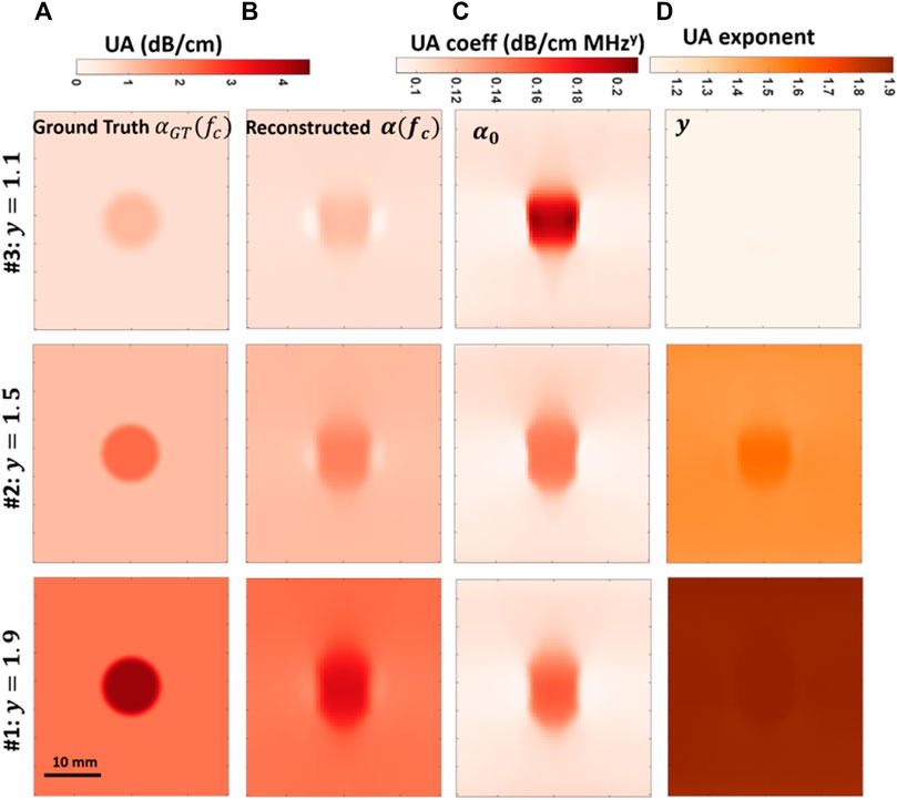
FIGURE 6. Comparison of frequency-dependent UA imaging for simulations varying the power-law dependence parameter y = {1.1, 1.5, 1.9}, with columns from left to right (A-D): ground-truth UA maps at center frequency 5 MHz; reconstructed UA maps at the center frequency; reconstructed α₀ maps; reconstructed y maps.

To quantify UA reconstructions, we report RMSE, CNR, and CRF in Table 1. Average RMSE of α(f_c) is 0.16 ± 0.09 dB/cm at center frequency 5 MHz. Considering the range of ground-truth SoS values, this demonstrates that an accurate reconstruction of UA is possible. With an RMSE of {0.04, 0.05, 0.06} respectively for prescribed y values {1.1, 1.5, 1.9}, the relative estimation error becomes below 3.3%, indicating a robust estimation of frequency exponent y. The contrast metrics CNR and CRF for α(f_c), α₀, and y demonstrate that the inclusions can be successfully distinguished in UA reconstructions, with a contrast similar to their prescribed ground-truth values.

3.2 Ex-Vivo Experiments Results

The SoS reconstruction results of the gelatin phantom and ex-vivo experiments are shown in Figure 7 with their corresponding B-Mode images in Figure 7A. Reconstructions of SoS maps at the center frequency are shown in Figure 7B, while reconstructed c₀ and c_y are shown in Figures 7C,D. The reconstructed results in Figure 7B were overlaid with inclusion markings annotated from the B-mode images. A clear contrast is visible in Figure 7 for all our proposed reconstructions. The reconstructed maps c (f_c) and c_y for gelatin and bovine tissue regions are consistent in phantoms #A and #B; i.e., the reconstructions show inverted images between these two phantoms, indicating that these quantities can be reproducibly used for tissue differentiation. From Figure 7C, it is observed that the tissue samples show much higher dispersion than in the simulations. This indicates the selection of frequency for SoS quantification being an important factor in practice. This also signifies the need for imaging C₀ and C_y to image the SoS of the targeted medium comprehensively. In other words, UA dispersion estimation can help both as additional parameters to characterize tissues and also for disambiguation of SoS measurement, which are seen here to be highly frequency dependent; also corroborating tissue observations in the literature, e.g. [33,39].

FIGURE 7

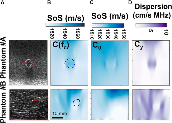
FIGURE 7. Comparison of frequency-dependent SoS imaging for phantom and ex-vivo tissues, with columns from left to right (A-D): B-mode image; c at the center frequency 5.2 MHz; reconstructed c₀ maps; reconstructed c_y maps.

The UA results of the gelatin phantom and ex-vivo experiments are shown in Figure 8. A clear contrast is visible for all the UA reconstructions using our proposed methods. Furthermore, all three reconstructed parameters between phantoms #A and #B are consistent, i.e., inclusion and background values inverted, showing reproducibility under different experimental settings. Axial edge artifacts, especially in y and α₀ maps were much reduced compared to results in [34] thanks to solving model parameters collectively in a closed form as in Eq. 9. The average and standard deviation values of SoS and UA obtained in gelatin and bovine tissue were tabulated along with CNR of the reconstructions in Table 2.

TABLE 2

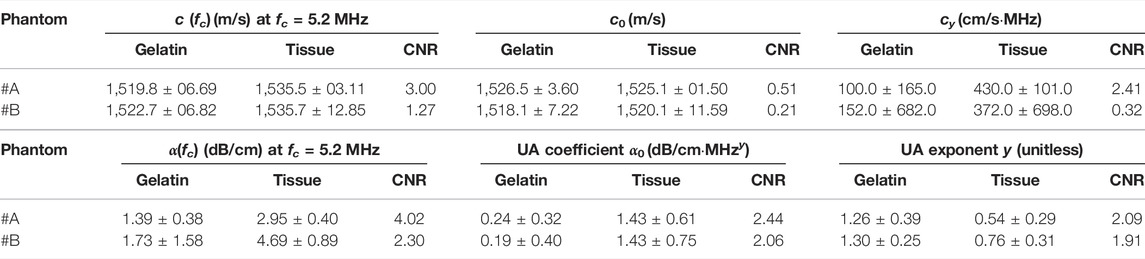
TABLE 2. Quantitative evaluation of SoS and UA model parameter reconstructions for ex-vivo experiments.

FIGURE 8

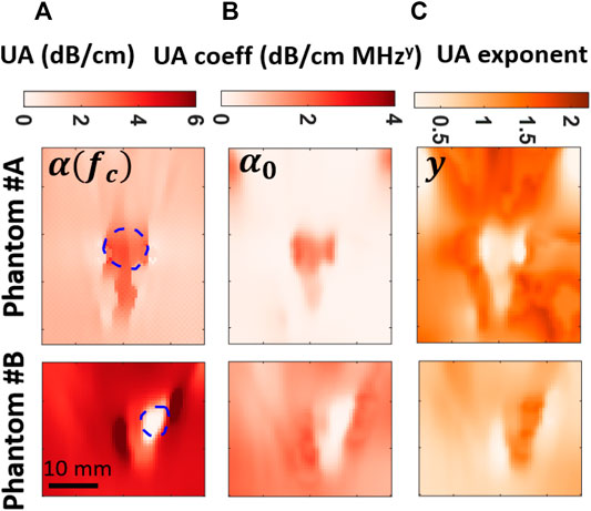
FIGURE 8. Comparison of frequency-dependent UA imaging for phantom and ex-vivo tissues, with columns from left to right (A-D): α at the center frequency 5.2 MHz; reconstructed α₀ maps; reconstructed y maps.

Using the relationship in Eq. 11, the complex bulk modulus of the gelatin phantom and ex-vivo tissues at ultrasound center frequency can be computed to be 2.31 + i (2.42 × 10^–3) GPa and 2.33 + i (10.01 × 10^–3) GPa, respectively. These values indicate 1) that the bulk loss modulus in both media is three orders of magnitude smaller than the bulk storage modulus; and 2) that although both media have similar bulk storage modulus, the bulk loss modulus in ex-vivo bovine tissue is ≈4 times higher than that of gelatin. This striking difference indicates that the complex bulk modulus may act as a new imaging biomarker, where the loss modulus component potentially having superior tissue differentiation compared to its storage component.

4 Conclusion

In this study, a novel method for reconstructing local SoS and UA maps as a function of frequency is introduced, through frequency domain analysis followed by a closed-form fitting of linear SoS and power-law UA dependency models. We first delineate the reflector profiles in multi-static data and compute Fourier transforms of these profiles to estimate phase and amplitude spectra. After calibrating these with water measurements, we use them to solve closed-form inverse problems over all frequencies to reconstruct SoS and UA frequency-dependent model parameters. We have studied these reconstructions with simulations and ex-vivo phantom studies, with our results indicating the following observations: The introduced SoS model parameters $c_{(f_c)}$ (SoS at center frequency), c₀ (SoS intercept), and c_y (SoS dispersion) were reconstructed with average RMSEs of 8.50 ± 0.24 m/s, 9.30 ± 0.31 m/s, and 47.6 ± 7.3 cm/s⋅MHz, respectively. These results show that c (f_c) and c₀ can be reconstructed with high accuracy, while c_y reconstructions were relatively poorer within the simulated low-dispersion regime. Still, the reconstructed c_y maps and their contrasts correlated with the ground-truth values. UA model parameters α(f_c), α₀, and y were reconstructed with average RMSEs of 0.16 ± 0.1 dB/cm, 0.01 ± 0dB/cm⋅MHz^y, and 0.05 ± 0.01, respectively, which indicate a high overall reconstruction accuracy using our proposed methods. From phantom and ex-vivo tissue sample experiments, the attenuation exponents in a gelatin-cellulose mixture and an ex-vivo bovine muscle sample were found to be, respectively, 1.3 and 0.6 on average. Linear dispersion of SoS in a gelatin-cellulose mixture and an ex-vivo bovine muscle sample were found to be, respectively, 1.3 and 4.0 m/s⋅MHz on average. Bulk loss modulus in bovine muscle sample was ≈4 times the bulk loss modulus in the gelatin-cellulose mixture. Our results show the feasibility of estimating spatial maps of frequency-dependent characteristics of SoS and UA, as well as the complex bulk modulus as potential imaging biomarkers.

Data Availability Statement

The original contributions presented in the study are included in the article/Supplementary Materials, further inquiries can be directed to the corresponding author.

Author Contributions

BC contributed with data processing, analysis and discussion of results, and manuscript drafting. RR contributed with supervision, conducting experiments, data processing, and discussion of results. OG contributed with supervision, analysis, discussion of results, and manuscript drafting.

Funding

Funding was provided by the Swiss National Science Foundation (SNSF).

Conflict of Interest

The authors declare that the research was conducted in the absence of any commercial or financial relationships that could be construed as a potential conflict of interest.

Publisher’s Note

All claims expressed in this article are solely those of the authors and do not necessarily represent those of their affiliated organizations, or those of the publisher, the editors and the reviewers. Any product that may be evaluated in this article, or claim that may be made by its manufacturer, is not guaranteed or endorsed by the publisher.

Footnotes

¹https://www.cs.ubc.ca/schmidtm/Software/minFunc.html.

References

1. Catheline S, Gennisson J-L, Delon G, Fink M, Sinkus R, Abouelkaram S, et al. Measurement of Viscoelastic Properties of Homogeneous Soft Solid Using Transient Elastography: An Inverse Problem Approach. J Acoust Soc Am (2004) 116:3734–41. doi:10.1121/1.1815075

PubMed Abstract | CrossRef Full Text | Google Scholar

2. Bercoff J, Tanter M, Fink M. Supersonic Shear Imaging: a New Technique for Soft Tissue Elasticity Mapping. IEEE Trans Ultrasonics, Ferroelectr Freq Control (2004) 51:396–409. doi:10.1109/tuffc.2004.1295425

CrossRef Full Text | Google Scholar

3. Fung Y-C. Biomechanics: Mechanical Properties of Living Tissues. Springer Science & Business Media (2013).

Google Scholar

4. Chen S, Fatemi M, Greenleaf JF. Quantifying Elasticity and Viscosity from Measurement of Shear Wave Speed Dispersion. J Acoust Soc Am (2004) 115:2781–5. doi:10.1121/1.1739480

PubMed Abstract | CrossRef Full Text | Google Scholar

5. Deffieux T, Montaldo G, Tanter M, Fink M. Shear Wave Spectroscopy for In Vivo Quantification of Human Soft Tissues Visco-Elasticity. IEEE Trans Med imaging (2008) 28:313–22. doi:10.1109/TMI.2008.925077

CrossRef Full Text | Google Scholar

6. Chen S, Urban MW, Pislaru C, Kinnick R, Zheng Y, Yao A, et al. Shearwave Dispersion Ultrasound Vibrometry (Sduv) for Measuring Tissue Elasticity and Viscosity. IEEE Trans ultrasonics, Ferroelectr Freq control (2009) 56:55–62. doi:10.1109/tuffc.2009.1005

CrossRef Full Text | Google Scholar

7. Nenadic IZ, Qiang B, Urban MW, Zhao H, Sanchez W, Greenleaf JF, et al. Attenuation Measuring Ultrasound Shearwave Elastography and In Vivo Application in Post-transplant Liver Patients. Phys Med Biol (2016) 62:484. doi:10.1088/1361-6560/aa4f6f

PubMed Abstract | CrossRef Full Text | Google Scholar

8. Budelli E, Brum J, Bernal M, Deffieux T, Tanter M, Lema P, et al. A Diffraction Correction for Storage and Loss Moduli Imaging Using Radiation Force Based Elastography. Phys Med Biol (2017) 62:91–106. doi:10.1088/1361-6560/62/1/91

PubMed Abstract | CrossRef Full Text | Google Scholar

9. Bernard S, Kazemirad S, Cloutier G. A Frequency-Shift Method to Measure Shear-Wave Attenuation in Soft Tissues. IEEE Trans ultrasonics, Ferroelectr Freq control (2016) 64:514–24.

PubMed Abstract | CrossRef Full Text | Google Scholar

10. Gennisson J-L, Rénier M, Catheline S, Barrière C, Bercoff J, Tanter M, et al. Acoustoelasticity in Soft Solids: Assessment of the Nonlinear Shear Modulus with the Acoustic Radiation Force. J Acoust Soc Am (2007) 122:3211–9. doi:10.1121/1.2793605

PubMed Abstract | CrossRef Full Text | Google Scholar

11. Latorre-Ossa H, Gennisson J-L, De Brosses E, Tanter M. Quantitative Imaging of Nonlinear Shear Modulus by Combining Static Elastography and Shear Wave Elastography. IEEE Trans ultrasonics, Ferroelectr Freq control (2012) 59:833–9. doi:10.1109/tuffc.2012.2262

CrossRef Full Text | Google Scholar

12. Otesteanu CF, Chintada BR, Sanabria SJ, Rominger M, Mazza E, Goksel O. Quantification of Nonlinear Elastic Constants Using Polynomials in Quasi-Incompressible Soft Solids. In: IEEE Int Ultrasonics Symposium (IUS) (2017). 1–4. doi:10.1109/ultsym.2017.8092332

CrossRef Full Text | Google Scholar

13. Bernal M, Chamming?s F, Couade M, Bercoff J, Tanter M, Gennisson J-L. In Vivo quantification of the Nonlinear Shear Modulus in Breast Lesions: Feasibility Study. IEEE Trans ultrasonics, Ferroelectr Freq control (2016) 63:101–9. doi:10.1109/tuffc.2015.2503601

PubMed Abstract | CrossRef Full Text | Google Scholar

14. Chintada BR, Rau R, Goksel O. Acoustoelasticity Analysis of Shear Waves for Nonlinear Biomechanical Characterization of Oil-Gelatin Phantoms. In: IEEE Int Ultrasonics Symposium (IUS) (2019). 423–6. doi:10.1109/ultsym.2019.8925670

CrossRef Full Text | Google Scholar

15. Otesteanu CF, Chintada BR, Rominger M, Sanabria S, Goksel O. Spectral Quantification of Nonlinear Elasticity Using Acousto-Elasticity and Shear-Wave Dispersion. IEEE Trans ultrasonics, Ferroelectr Freq control (2019) 66:1845–55. doi:10.1109/tuffc.2019.2933952

PubMed Abstract | CrossRef Full Text | Google Scholar

16. Chintada BR, Rau R, Goksel O. Nonlinear Characterization of Tissue Viscoelasticity with Acoustoelastic Attenuation of Shear Waves. IEEE Trans Ultrasonics, Ferroelectr Freq Control (2021) 69:38–53.

Google Scholar

17. Goswami S, Ahmed R, Doyley MM, McAleavey SA. Local Spectral Nonlinear Elasticity Imaging: Contrast Enhancement in Heterogeneous Elastograms Based on Viscoelastic Nonlinear Characterizations. In: IEEE Int Ultrasonics Symposium (IUS) (2020). 1–3. doi:10.1109/ius46767.2020.9251283

CrossRef Full Text | Google Scholar

18. Duric N. Detection of Breast Cancer with Ultrasound Tomography: First Results with the Computed Ultrasound Risk Evaluation (Cure) Prototype. Med Phys (2007) 34:773–85. doi:10.1118/1.2432161

PubMed Abstract | CrossRef Full Text | Google Scholar

19. Greenleaf JF, Bahn RC. Clinical Imaging with Transmissive Ultrasonic Computerized Tomography. IEEE Trans Biomed Eng (1981) 177–85. doi:10.1109/tbme.1981.324789

PubMed Abstract | CrossRef Full Text | Google Scholar

20. Gemmeke H, Ruiter N. 3d Ultrasound Computer Tomography for Medical Imaging. Nucl Instrum Methods Phys Res Sect A Accel Spectrom Detect Assoc Equip (2007) 580:1057–65. doi:10.1016/j.nima.2007.06.116

CrossRef Full Text | Google Scholar

21. Jaeger M, Held G, Peeters S, Preisser S, Grünig M, Frenz M. Computed Ultrasound Tomography in Echo Mode for Imaging Speed of Sound Using Pulse-Echo Sonography: Proof of Principle. Ultrasound Med Biol (2015) 41:235–50. doi:10.1016/j.ultrasmedbio.2014.05.019

PubMed Abstract | CrossRef Full Text | Google Scholar

22. Sanabria SJ, Ozkan E, Rominger M, Goksel O. Spatial Domain Reconstruction for Imaging Speed-Of-Sound with Pulse-Echo Ultrasound: Simulation and In Vivo Study. Phys Med Biol (2018) 63:215015. doi:10.1088/1361-6560/aae2fb

PubMed Abstract | CrossRef Full Text | Google Scholar

23. Rau R, Schweizer D, Vishnevskiy V, Goksel O. Speed-of-sound Imaging Using Diverging Waves. Int J Comput Assisted Radiology Surg (2021) 16:1201–11. doi:10.1007/s11548-021-02426-w

CrossRef Full Text | Google Scholar

24. Krueger M, Burow V, Hiltawsky K, Ermert H. Limited Angle Ultrasonic Transmission Tomography of the Compressed Female Breast. In: IEEE Int Ultrasonics Symposium, 2 (1998). 1345–8.

Google Scholar

25. Sanabria SJ, Rominger MB, Goksel O. Speed-of-sound Imaging Based on Reflector Delineation. IEEE Trans Biomed Eng (2018) 66:1949–62.

PubMed Abstract | CrossRef Full Text | Google Scholar

26. Parker KJ, Waag RC. Measurement of Ultrasonic Attenuation within Regions Selected from B-Scan Images. IEEE Trans Biomed Eng (1983) 431–7. doi:10.1109/tbme.1983.325148

PubMed Abstract | CrossRef Full Text | Google Scholar

27. Coila AL, Lavarello R. Regularized Spectral Log Difference Technique for Ultrasonic Attenuation Imaging. IEEE Trans ultrasonics, Ferroelectr Freq control (2017) 65:378–89. doi:10.1109/TUFFC.2017.2719962

PubMed Abstract | CrossRef Full Text | Google Scholar

28. Vajihi Z, Rosado-Mendez IM, Hall TJ, Rivaz H. Low Variance Estimation of Backscatter Quantitative Ultrasound Parameters Using Dynamic Programming. IEEE Trans ultrasonics, Ferroelectr Freq control (2018) 65:2042–53. doi:10.1109/tuffc.2018.2869810

PubMed Abstract | CrossRef Full Text | Google Scholar

29. Gong P, Song P, Huang C, Trzasko J, Chen S. System-independent Ultrasound Attenuation Coefficient Estimation Using Spectra Normalization. IEEE Trans ultrasonics, Ferroelectr Freq control (2019) 66:867–75. doi:10.1109/tuffc.2019.2903010

PubMed Abstract | CrossRef Full Text | Google Scholar

30. Huang S-W, Li P-C. Ultrasonic Computed Tomography Reconstruction of the Attenuation Coefficient Using a Linear Array. IEEE Trans ultrasonics, Ferroelectr Freq control (2005) 52:2011–22. doi:10.1109/tuffc.2005.1561670

CrossRef Full Text | Google Scholar

31. Chang C-H, Huang S-W, Yang H-C, Chou Y-H, Li P-C. Reconstruction of Ultrasonic Sound Velocity and Attenuation Coefficient Using Linear Arrays: Clinical Assessment. Ultrasound Med Biol (2007) 33:1681–7. doi:10.1016/j.ultrasmedbio.2007.05.012

PubMed Abstract | CrossRef Full Text | Google Scholar

32. Rau R, Unal O, Schweizer D, Vishnevskiy V, Goksel O. Attenuation Imaging with Pulse-Echo Ultrasound Based on an Acoustic Reflector. In: Medical Image Computing and Computer Assisted Intervention. MICCAI (2019). 601–9. doi:10.1007/978-3-030-32254-0_67

CrossRef Full Text | Google Scholar

33. Bamber JC, Hill CR. Acoustic Properties of Normal and Cancerous Human Liver-I. Dependence on Pathological Condition. Ultrasound Med Biol (1981) 7:121–33. doi:10.1016/0301-5629(81)90001-6

PubMed Abstract | CrossRef Full Text | Google Scholar

34. Rau R, Unal O, Schweizer D, Vishnevskiy V, Goksel O. Frequency-dependent Attenuation Reconstruction with an Acoustic Reflector. Med Image Anal (2021) 67:101875. doi:10.1016/j.media.2020.101875

PubMed Abstract | CrossRef Full Text | Google Scholar

35. Mast TD, Hinkelman LM, Metlay LA, Orr MJ, Waag RC. Simulation of Ultrasonic Pulse Propagation, Distortion, and Attenuation in the Human Chest Wall. J Acoust Soc Am (1999) 106:3665–77. doi:10.1121/1.428209

PubMed Abstract | CrossRef Full Text | Google Scholar

36. Sehgal C, Brown G, Bahn R, Greenleaf J. Measurement and Use of Acoustic Nonlinearity and Sound Speed to Estimate Composition of Excised Livers. Ultrasound Med Biol (1986) 12:865–74. doi:10.1016/0301-5629(86)90004-9

PubMed Abstract | CrossRef Full Text | Google Scholar

37. Mast TD. Empirical Relationships between Acoustic Parameters in Human Soft Tissues. Acoust Res Lett Online (2000) 1:37–42. doi:10.1121/1.1336896

CrossRef Full Text | Google Scholar

38. Treeby BE, Zhang EZ, Thomas AS, Cox BT. Measurement of the Ultrasound Attenuation and Dispersion in Whole Human Blood and its Components from 0–70 Mhz. Ultrasound Med Biol (2011) 37:289–300. doi:10.1016/j.ultrasmedbio.2010.10.020

PubMed Abstract | CrossRef Full Text | Google Scholar

39. Duck FA. Physical Properties of Tissues: A Comprehensive Reference Book. Academic Press (2013).

Google Scholar

40. Kremkau FW, Barnes RW, McGraw CP. Ultrasonic Attenuation and Propagation Speed in Normal Human Brain. J Acoust Soc Am (1981) 70:29–38. doi:10.1121/1.386578

CrossRef Full Text | Google Scholar

41. Chintada BR, Rau R, Goksel O. Time of Arrival Delineation in Echo Traces for Reflection Ultrasound Tomography. In: IEEE Int Symp on Biomedical Imaging. ISBI (2021). 1342–5. doi:10.1109/isbi48211.2021.9433846

CrossRef Full Text | Google Scholar

42. Del Grosso V, Mader C. Speed of Sound in Pure Water. J Acoust Soc Am (1972) 52:1442–6. doi:10.1121/1.1913258

CrossRef Full Text | Google Scholar

43. Krautkrämer J, Krautkrämer H. Ultrasonic Testing of Materials. Springer Science & Business Media (2013).

Google Scholar

44. Fu H, Ng MK, Nikolova M, Barlow JL. Efficient Minimization Methods of Mixed L2-L1 and L1-L1 Norms for Image Restoration. SIAM J Sci Comput (2006) 27:1881–902. doi:10.1137/040615079

CrossRef Full Text | Google Scholar

45. Sanabria SJ, Goksel O. Hand-held Sound-Speed Imaging Based on Ultrasound Reflector Delineation. In: Int Conf on Medical Image Computing and Computer-Assisted Intervention (MICCAI) (2016). 568–76. doi:10.1007/978-3-319-46720-7_66

CrossRef Full Text | Google Scholar

46. Broyden CG. The Convergence of a Class of Double-Rank Minimization Algorithms 1. General Considerations. IMA J Appl Math (1970) 6:76–90. doi:10.1093/imamat/6.1.76

CrossRef Full Text | Google Scholar

47. Fletcher R. A New Approach to Variable Metric Algorithms. Comput J (1970) 13:317–22. doi:10.1093/comjnl/13.3.317

CrossRef Full Text | Google Scholar

48. Goldfarb D. A Family of Variable-Metric Methods Derived by Variational Means. Math Comput (1970) 24:23–6. doi:10.1090/s0025-5718-1970-0258249-6

CrossRef Full Text | Google Scholar

49. Shanno DF. Conditioning of Quasi-Newton Methods for Function Minimization. Math Comput (1970) 24:647–56. doi:10.1090/s0025-5718-1970-0274029-x

CrossRef Full Text | Google Scholar

50. Waters KR, Hughes MS, Mobley J, Brandenburger GH, Miller JG. On the Applicability of Kramers–Krönig Relations for Ultrasonic Attenuation Obeying a Frequency Power Law. J Acoust Soc Am (2000) 108:556–63. doi:10.1121/1.429586

PubMed Abstract | CrossRef Full Text | Google Scholar

51. Waters KR, Mobley J, Miller JG. Causality-imposed (Kramers-kronig) Relationships between Attenuation and Dispersion. IEEE Trans ultrasonics, Ferroelectr Freq control (2005) 52:822–3. doi:10.1109/tuffc.2005.1503968

PubMed Abstract | CrossRef Full Text | Google Scholar

52. Treeby BE, Cox BT. Modeling Power Law Absorption and Dispersion for Acoustic Propagation Using the Fractional Laplacian. J Acoust Soc Am (2010) 127:2741–8. doi:10.1121/1.3377056

PubMed Abstract | CrossRef Full Text | Google Scholar

53. Barry CT, Mills B, Hah Z, Mooney RA, Ryan CK, Rubens DJ. Shear Wave Dispersion Measures Liver Steatosis. Ultrasound Med Biol (2012) 38:175–82. doi:10.1016/j.ultrasmedbio.2011.10.019

PubMed Abstract | CrossRef Full Text | Google Scholar

54. Treeby BE, Cox BT. K-Wave: Matlab Toolbox for the Simulation and Reconstruction of Photoacoustic Wave Fields. J Biomed Opt (2010) 15:021314. doi:10.1117/1.3360308

PubMed Abstract | CrossRef Full Text | Google Scholar

55. Fischler MA, Bolles RC. Random Sample Consensus: a Paradigm for Model Fitting with Applications to Image Analysis and Automated Cartography. Commun ACM (1981) 24:381–95. doi:10.1145/358669.358692

CrossRef Full Text | Google Scholar

56. Kass M, Witkin A, Terzopoulos D. Snakes: Active Contour Models. Int J Comp Vis (1988) 1:321–31. doi:10.1007/bf00133570

CrossRef Full Text | Google Scholar

57. Vishnevskiy V, Sanabria SJ, Goksel O. Image Reconstruction via Variational Network for Real-Time Hand-Held Sound-Speed Imaging. In: International workshop on machine learning for medical image reconstruction. Springer (2018). 120–8. doi:10.1007/978-3-030-00129-2_14

CrossRef Full Text | Google Scholar

58. Vishnevskiy V, Rau R, Goksel O. Deep Variational Networks with Exponential Weighting for Learning Computed Tomography. In: International Conference on Medical Image Computing and Computer-Assisted Intervention. Springer (2019). 310–8. doi:10.1007/978-3-030-32226-7_35

CrossRef Full Text | Google Scholar