Detecting Local Opinion Leader in Semantic Social Networks: A Community-Based Approach

Online social networks have been incorporated into people’s work and daily lives as social media and services continue to develop. Opinion leaders are social media activists who forward and filter messages in mass communication. Therefore, competent monitoring of opinion leaders may, to some extent, influence the spread and growth of public opinion. Most traditional opinion leader mining approaches focus solely on the user’s network structure, neglecting the significance and role of semantic information in the generation of opinion leaders. Furthermore, these methods rank the influence of users globally and lack effectiveness in detecting local opinion leaders with low influence. This paper presents a community-based opinion leader mining approach in semantic social networks to address these issues. Firstly, we present a new node semantic feature representation method and community detection algorithm to generate the local public opinion circle. Then, a novel influence calculation method is proposed to find local opinion leaders by combining the global structure of the network and local structure of the public opinion circle. Finally, nodes with high comprehensive influence are identified as opinion leaders. Experiments on real social networks indicate that the proposed method can accurately measure global and local influence in social networks, as well as increase the accuracy of local opinion leader mining.

1 Introduction

The social network is a complex structure made up of people or entities who are linked together by some kind of relationship or shared interest (friendship, professional relationship, kinship, etc.) [1]. As tens of thousands of people around the world utilize social networks to interact, the Internet can continue to share an enormous quantity of data, resulting in the exponential expansion of social media and online social networks (e.g., Facebook, Twitter, Weibo) in recent years. Simultaneously, online social networks have grown in popularity as a result of their convenience, openness, anonymity, and virtual character, and have steadily evolved into a major carrier of online opinion and information distribution [2–5]. Texts, emojis, hashtags, and gif videos all contribute to the propagation of public opinion on social media [6]. As a result, online public opinion has evolved into a distinct form of public opinion with increasing social clout.

Most studies on online public opinion, including online opinion mining, dissemination patterns, and data mining, currently focus on the spread of online public opinion on social media [7–9]. The status of users in social networks is unequal, those in the center play a leading and driving role in the development of online public opinion, while those in the periphery are easily influenced by other factors (Aleahmad et al., 2016). Internet opinion leaders are often at the center, and their communication can easily push certain events to the forefront of the public opinion wave (Walter and Brüggemann, 2020). Public opinion leadership has the potential to not only actively guide public life, but also to trigger a wide range of negative emotions [12]. As a result, mining public opinion leaders is an important factor of guiding correct public opinion and sustaining network order.

Community detection is the process of dividing social users into tightly connected and highly relevant groups so that each group can be well separated from the others (Chunaev, 2020). Community detection has important applications in the fields of social network analysis, data mining, spatial database technology, statistics, biology, and smart grids [14–18]. This paper uses community detection to build a public opinion circle of users with the same ideas and opinions in social networks. Different from directly detecting opinion communities by leveraging connections between nodes [19], we use the semantic cohesiveness [20] and structural compactness of the community to further enhance the impact and effect of opinion leaders in the local environment.

Thanks to the development of online web technology, we can easily extract semantic information released by any individual from popular semantic social networks such as Facebook, Twitter, and Sina Weibo. At present, online opinion leaders detection mostly uses user behavior analysis [21,22], text semantic or sentiment analysis [23,24], node centrality analysis [25,26]. These methods, however, do not adequately account for the complexity of individuals in the local environment, and there is a lack of effective identification of opinion leaders with strong local influence.

To improve the performance of online opinion leader mining, we propose using the individual’s local structure to weight the influence score when mining opinion leaders. Firstly, an LDA topic model is introduced to obtain the topic distribution of semantic information of users and complete the construction of social networks; then a community detection algorithm based on σ-norm is proposed to obtain the community structure of social networks and form multiple opinion circles; Finally, using the graph structure of the community, we propose an influence calculation method based on the global and local structure of the graph to detect the opinion leaders of social networks. Experiments on real social networks show that the method proposed in this paper can extract online opinion leaders accurately and effectively.

In summary, the contributions of this paper are as follows:

(1) We propose a new opinion leader mining method that considers both semantic information and network structure of users.

(2) We construct a new node semantic feature representation method by computing the similarity between user documents and global topics to map user semantic to topology spaces.

(3) A community detection algorithm based on σ-norm is proposed, which can accurately output high-quality community partition results by exploiting the robustness of l21-norm and F-norm.

(4) We present a new influence calculation method that combines the global and local structure of the graph, successfully avoiding the impact of global high-influence nodes in local influence calculation.

2 Semantic Information Discovery of Social Network

In social networks, users express their views or opinions in response to various message. We define the social network as $G=\left(V,E,D\right)$, where V is the set of nodes, E is the set of edges, D represents the semantic information. The semantic information published by user node v ∈ V is d ∈ D. Meanwhile, we abstract semantic information into topics and topic keywords and use them as feature attributes of nodes. Afterward, the connections e ∈ E are established based on the similarity of the topics to which the nodes belong. We use the LDA topic model to process node semantic information.

2.1 LDA Representation of Semantic Information

LDA (Latent Dirichlet Allocation) is a three-level Bayesian model for document generation, which considers an article as having multiple topics, and each topic corresponds to a different word. Figure 1 shows the semantic information published by users in the social network, which contains three documents with the words marked with different colors. For example, words related to the biological environment are “coronavirus” and “vaccines,” which are marked with green; words related to political life are “government” and “official,” which are marked with yellow; words related to economy are “economy” and “opening,” which are marked with blue. If all the words in the document are marked, it can be found that each post mixes different topics in different proportions. For example, the first post mixes bioenvironmental and political themes, and the bioenvironmental theme has a higher proportion. With this idea, the topic distribution of semantic information in social networks can be extracted and the exploration of semantic information can be realized.

FIGURE 1

FIGURE 1. LDA model for document generation process of semantic information published by users in social networks.

The mathematical notation involved in the LDA topic model is shown in Table 1, and it is generated for each node as follows:

(1) θ_d ∼ Dirichlet(α): The topic distribution θ_d of document d follows the Dirichlet distribution with hyperparameter α, where α determines the proportion of the distribution of topics in document d.

(2) β_z ∼ Dirichlet(η): The word distribution β_z of topic z follows the Dirichlet distribution with hyperparameter η, where η determines the proportion of words distributed in the topic.

(3) $z_i\mid {\theta }_d\sim Multinomial\left({\theta }_d\right)$: The topic number z_i follows a polynomial distribution under the topic distribution θ_d.

(4) $w_i\mid z_i,{\beta }_{z_i}\sim Multinomial\left({\beta }_{z_i}\right)$: The probability of occurrence of keyword w_i in topic z_i follows a polynomial distribution under word distribution ${\beta }_{z_i}$.

TABLE 1

TABLE 1. Description of notations.

In summary, n documents will correspond to n independent Dirichlet-Multinomial conjugate structures, and K topics will correspond to K independent Dirichlet-Multinomial conjugate structures. Use α to generate topic distribution θ, and topic distribution θ determines the specific topic. Use η to generate word distribution β, which determines the specific keyword, i.e

$\begin{array}{cc}\hfill & \alpha ⃗\to {\vec{\theta }}_d\to z⃗\hfill \\ \hfill & \eta ⃗\to {\beta ⃗}_{z_i}\to w⃗\hfill \end{array}(1)$

2.2 Gibbs Sampling Process

Gibbs sampling is a Markov-Chain-Monte-Carlo (MCMC) method and is widely used in probability inference (Su et al., 2018). Gibbs sampling approximately samples a group of random variables from a complex joint distribution to obtain the conditional probability distribution of each characteristic dimension. Specifically for the LDA model, our goal is to obtain the overall probability distribution $z⃗$ and $w⃗$, corresponding to each z_i and w_i, i.e., topic distribution of documents and word distribution of topics.

Using the relationship existing in Eq. 1, the joint probability distribution $p(w⃗,z⃗|\alpha ⃗,\eta ⃗)$ of topics and words can be obtained as follows:

$\begin{array}{c}p\left(\vec{w},z⃗\right)\propto p\left(w⃗,z⃗|\alpha ⃗,\eta ⃗\right)\hfill \\ =p\left(z⃗|\alpha ⃗\right)p\left(w⃗|z⃗,\eta ⃗\right)=\prod _{d=1}^{\left|D\right|}\frac{\mathrm{\Delta }\left({n⃗}_d+\alpha ⃗\right)}{\mathrm{\Delta }\left(\alpha ⃗\right)}\prod _{t=1}^T\frac{\mathrm{\Delta }\left({n⃗}_t+\eta ⃗\right)}{\mathrm{\Delta }\left(\vec{\eta }\right)}\hfill \end{array}(2)$

Where $\mathrm{\Delta }(\alpha ⃗)$, $\mathrm{\Delta }(\eta ⃗)$ are the normalization parameters, ${n⃗}_d=\left(n_d^{(1)},n_d^{(2)},\dots ,n_d^{(T)}\right)$, $n_d^{(t)}$ is the number of occurrences of the word for the tth topic in the dth document; ${n⃗}_t=\left(n_t^{(1)},n_t^{(2)},\dots ,n_t^{(H)}\right)$, $n_t^{(h)}$ is the number of occurrences of the h-th word in the t-th topic. Given the conditional distribution $p(z⃗|w⃗)$ of the observable variable $w⃗$ under the hidden content $\vec{z}$, Bayesian analysis can be performed on it using the joint distribution (Eq. 2). The Bayesian relationship between $z⃗$ and $\vec{w}$ is expressed as:

$\begin{array}{c}p\left(z_i=o|{\vec{z}}_{\neg i},\vec{w}\right)\propto p\left(z_i=o,w_i=y|{\vec{z}}_{\neg i},{\vec{w}}_{\neg i}\right)\hfill \\ =\int p\left(z_i=o,{\vec{\theta }}_d\mid {\vec{w}}_{\neg i},{\vec{z}}_{\neg i}\right)p\left(w_i=y,{\vec{\beta }}_{z_i}\mid {\vec{w}}_{\neg i},{\vec{z}}_{\neg i}\right)d{\vec{\theta }}_{d}d{\vec{\beta }}_{z_i}\hfill \\ =\int p\left(z_i=o\mid {\vec{\theta }}_d\right)p\left({\vec{\theta }}_d\mid {\vec{w}}_{\neg i},{\vec{z}}_{\neg i}\right)p\left(w_i=y\mid {\vec{\beta }}_{z_i}\right)p\left({\vec{\beta }}_{z_i}\mid {\vec{w}}_{\neg i},{\vec{z}}_{-i}\right)d{\vec{\theta }}_{d}d{\vec{\beta }}_{z_i}\hfill \end{array}(3)$

When z_i = o, w_i = y, the probability $p\left(z_i=o,w_i=y|{\vec{z}}_{\neg i},{\vec{w}}_{\neg i}\right)$ only involves the conjugate distribution of the dth document and the tth topic under the Dirichlet-Multinomial model. where y is one of the keywords in w; o corresponding to y, is one of the topics in z; ${\vec{w}}_{\neg i},{\vec{z}}_{\neg i}$ represents the corresponding topic distribution and word distribution after removing topics and words with subscript i; the posterior distributions of ${\vec{\theta }}_d$ and ${\vec{\beta }}_{z_i}$ can be calculated by the following equation:

$\begin{array}{c}p\left({\vec{\theta }}_d\mid {\vec{w}}_{\neg i},{\vec{z}}_{\neg i}\right)=Dirichlet\left({\vec{\theta }}_d\mid {\vec{n}}_{d,\neg i}+\alpha ⃗\right)\hfill \\ p\left({\beta ⃗}_{z_i}\mid {w⃗}_{\neg i},{z⃗}_{\neg i}\right)=Dirichlet\left({\beta ⃗}_{z_i}\mid {n⃗}_{t,\neg i}+\eta ⃗\right)\hfill \end{array}(4)$

Thus, Eq. 3 can be reduced to:

$\begin{array}{c}\int p\left(z_i=o|{\theta ⃗}_d\right)Dirichlet\left({\theta ⃗}_d|{n⃗}_{d,\neg i}+\alpha ⃗\right)d{\vec{\theta }}_d\cdot \int p\left(w_i=y\mid {\vec{\beta }}_{z_i}\right)Dirichlet\left({\vec{\beta }}_{z_i}|{n⃗}_{t,\neg i}+\eta ⃗\right)d{\vec{\beta }}_{z_i}=\frac{n_{d,\neg i}^o+{\alpha }_o}{\sum _{t=1}^T{n}_{d,\neg i}^t+{\alpha }_t}\cdot \frac{n_{k,\neg i}^y+{\eta }_y}{\sum _{h=1}^H{n}_{k,\neg i}^h+{\eta }_h}\hfill \\ \Rightarrow p\left(z_i=o|w⃗,{z⃗}_{\neg i}\right)\propto \frac{n_{d,\neg i}^o+{\alpha }_o}{\sum _{t=1}^T{n}_{d,\neg i}^t+{\alpha }_t}\cdot \frac{n_{k,\neg i}^y+{\eta }_y}{\sum _{h=1}^H{n}_{k,\neg i}^h+{\eta }_h}\hfill \end{array}(5)$

Where α_o(α_t) is the hyperparameter α of the topic distribution corresponding to the topic of o(t). η_y(η_h) is the hyperparameter η of the word distribution corresponding to the keyword of y(h). $n_{d,-i}^k$ is the number of topics when z_i = o. $n_{k,\neg i}^t$ is the number of keywords when w_i = y.

Gibbs sampling is performed on the topics of all words by Eq. 5, and when the sampling converges, the topics corresponding to all words are obtained; then, according to the correspondence between the sampled words and topics, we can get the topic distribution θ_d of each document and the distribution β_k of keywords in each topic.

3 Community Detection Based on Topic Distribution

3.1 Node Representation

In this paper, the semantic information corresponding to the user nodes v_i in the social network is used as the document d_i to generate the topic distribution ${\theta }_{d_i}$. Therefore, each node is represented as a K-dimensional vector and is equal to the topic probability distribution of the node corresponding to the document. The set of all node vectors is formed into a data matrix X of K × n to implement the node representation, where the matrix X is calculated as follows:

$x_{i,j}=\left\{\begin{array}{cc}\hfill 0,\hfill & \hfill z_j=0\hfill \\ \hfill {\theta }_{d_i}^{z_j},\hfill & \hfill z_j\ne 0\hfill \end{array}\right.(6)$

In Eq. 6, x_i,j denotes the value of the ith row and jth column of the data matrix X, and ${\theta }_{d_i}^{z_j}$ denotes the probability that document d_i belongs to the jth topic. Therefore, when the probability of the jth topic in the topic distribution ${\theta }_{d_i}$ is zero, X = 0; when the probability of the jth topic in the topic distribution ${\theta }_{d_i}$ is non-zero, $x_{i,j}={\theta }_{d_i}^{z_j}$, which constitutes the user node vector, and the data matrix X is obtained to complete the node representation.

3.2 Establishing Associations

Calculating the similarity between node vectors can establish association for nodes. Two users with high correlation in a social network will correspond to a large similarity value, low correlation users will correspond to a low similarity value, and uncorrelated users will have zero similarity value. Commonly used similarity calculation methods include cosine similarity, Pearson correlation coefficient, and Gaussian kernel similarity calculation methods. These methods are sensitive to noise and outliers and are easy to ignore the local structure of data and the size of the vector itself. Therefore, this paper chooses a data similarity matrix learning method based on sparse representation [28] that is robust to noise kernel outliers in the data [29] and fits the requirement of connecting social network users. We can obtain the similarity matrix between users in a social network by solving the following equation:

$\begin{array}{c}{\min }_{a_{i,j}}{a}_{i,j}{‖{x⃗}_i-{x⃗}_j‖}_2^2+\epsilon \sum _i^n\sum _j^n{a}_{i,j}\hfill \\ s.t.{\mathbf{1}}^T{a⃗}_i=1,a_{i,i}=0,a_{i,j}\ge 0\hfill \end{array}(7)$

Where a_i,j is the value of the ith row and jth column of the similarity matrix A, A ∈ R^n×n. n is the number of users in the social network. ${a⃗}_i$ is the vector of the ith row of A, which represents the similarity value between user i and other users. ɛ is the sparse adjustment factor. 1 is a vector with all values of 1, constraint ${\mathbf{1}}^T{a⃗}_i=1$ makes the second term in Eq. 7 to be constant. That is, the constraint ${\mathbf{1}}^T{a⃗}_i=1$ is equivalent to a sparse constraint on A.

After calculation and derivation, the following results can be obtained:

${\widehat{a}}_{i,j}=\left\{\begin{array}{cc}\hfill \frac{c_{i,m+1}-c_{i,j}}{m{c}_{i,m+1}-\sum _{h=1}^m{c}_{i,h}}\hfill & \hfill j\le m\hfill \\ \hfill 0\hfill & \hfill j>m\hfill \end{array}\right.(8)$

Where $c_{i,j}={‖x_i-x_j‖}_2^2$, Sort them from small to large so that the learning of c_i,j satisfies ${\widehat{c}}_{i,m}>0$, and ${\widehat{c}}_{i,m+1}=0$. m is the number of adaptive neighbors. The similarity matrix calculated using cosine similarity, Pearson correlation coefficient, and other methods is usually presented in the form of fully connected or K-nearest neighbors. The similarity matrix A calculated by Eq. 8 can adapt to the number of neighbors m of users in the social network, compensating for the disadvantage that community detection requires high node similarity. This will improve the quality of the community structure and, as a result, accurately detect network opinion leaders.

3.3 Constructing Community Detection Algorithm

Loss function is usually constructed using the l1-norm and the l2-norm. The loss function constructed using the l1-norm has the disadvantage of being insensitive to larger outliers but sensitive to smaller ones; the l2-norm does the opposite. σ-norm [30] neutralizes the above two problems and is defined as follows:

${‖x⃗‖}_{\sigma }=\sum _i^n\frac{\left(1+\sigma \right)x_i^2}{x_i^2+\sigma }(9)$

Where σ is the adaptive parameter. The generalization of the vector $x⃗$ into matrix X is equivalent to neutralizing the l21-norm and F-norm of the matrix. Thus, the σ-norm takes advantage of the robustness of the l21-norm and F-norm precisely for both large and small outliers, and ${‖X‖}_{\sigma }$ is nonnegative, convex, and quadratically differentiable.

${‖X‖}_{\sigma }=\sum _i^n\frac{\left(1+\sigma \right){‖{x⃗}_i‖}_2^2}{{‖{x⃗}_i‖}_2+\sigma }(10)$

After constructing the similarity matrix A of the social network by Eq. 8, we introduce the rank constraint and propose the following objective function:

$\begin{array}{c}{\min }_U{‖A-U‖}_{\sigma }\hfill \\ s.t.{\mathbf{1}}^T{u⃗}_i=1,u_{i,j}\ge 0,\mathrm{rank}\left(L\right)=n-k\hfill \end{array}(11)$

In Eq. 11, U is the target matrix obtained from learning, due to the introduction of rank constraint, the target matrix U will have k connected components, so it can directly output the k community structures of the social network; L is the Laplace matrix of U; L = R − S, where R is diagonal matrix, $r_{ii}=\sum _{j=1}^n{u}_{i,j}$; and $S=\left(U^T+U\right)/2$; the constraint ${\mathbf{1}}^T{u⃗}_i=1$ is set to avoid anomalous nodes (without any neighbors), so that the sum of each row of U is 1.

However, the dependence of L on the variable S and the nonlinearity of the rank constraint leads to the difficulty in solving Eq. 11. To solve this puzzle, we define ${\lambda }_i\left(L\right)$ to denote the ith smallest eigenvalue of L. Since the matrix L is a symmetric semi-positive definite matrix, the eigenvalues of L are real and non-negative [31], so there exists ${\lambda }_i\left(L\right)\ge 0$. Then, if the first k smallest eigenvalues of L satisfy $\sum _{i=1}^k{\lambda }_i\left(L\right)=0$, the rank constraint rank(L) = n − k is achieved, and Eq. 11 can be expressed as:

$\begin{array}{c}{\min }_S{‖A-U‖}_{\sigma }+\rho \sum _{i=1}^k{\lambda }_i\left(L\right)\hfill \\ s.t.{\mathbf{1}}^T{u⃗}_i=1,u_{i,j}\ge 0\hfill \end{array}(12)$

Where ρ is a balancing factor that can increase or decrease its value to cope with the cases that the connected components of the target matrix U are greater or less than k until k connected components of U exist. According to Fan’s study [32], there is the following theorem:

$\begin{array}{c}\sum _{i=1}^k{\lambda }_i\left(L\right)=\min \mathrm{Tr}\left(F^{T}LF\right)\hfill \\ s.t.F^{T}F=I\hfill \end{array}(13)$

Where $F=\left\{{f⃗}_1,{f⃗}_2,\dots ,{f⃗}_k\right\}$ is the clustering indicator matrix, which is used to output clustering results in spectral clustering; I is the identity matrix. Substituting Eq. 13 into Eq. 12 gives:

$\begin{array}{c}{\min }_{U,F}{‖A-U‖}_{\sigma }+\rho \mathrm{Tr}\left(F^{T}LF\right)\hfill \\ s.t.{\mathbf{1}}^T{u⃗}_i=1,u_{i,j}\ge 0,F^{T}F=I\hfill \end{array}(14)$

Eq. 14 is the final objective function, where the objective matrix U has k connected components, so that the final community detection results can be obtained directly using this algorithm.

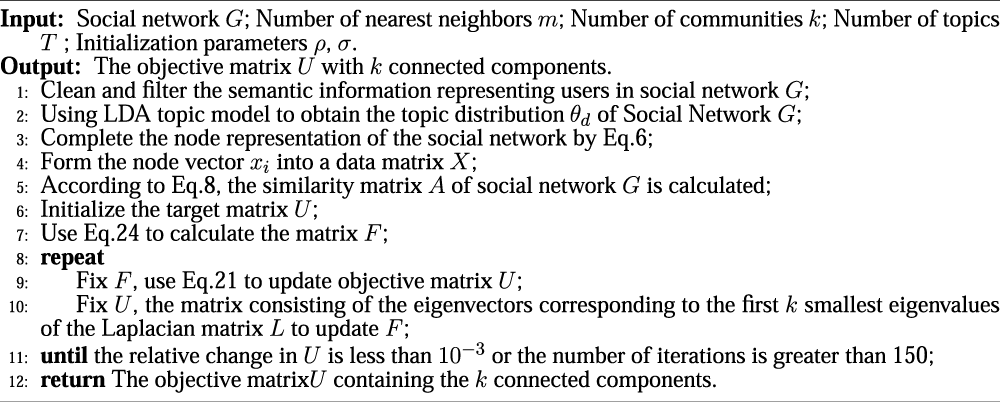
3.4 Algorithm Optimization

We introduce an iterative optimization algorithm for solving Eq. 14 and the target variable U therein. Since the target variable U and other variables F are coupled in one equation, solving Eq. 14 and deriving all variables at once is a challenging problem. In addition, the constraints in the objective function are not smooth. Assuming that A, F has been obtained, the target variable U can be computed using ALM (Augmented Lagrange Multiplier). ALM performs superiorly on matrix analysis problems [33]. Similarly, when the variable U is fixed, F can be computed. The detailed computational strategy is as follows:

(1) Keep F fixed, update U.

When F is fixed, using the Laplace matrix nature $\sum _{i,j}\frac{1}{2}{‖{f⃗}_i-{\vec{f}}_j‖}_2^2{s}_{i,j}=\mathrm{Tr}\left(F^{T}LF\right)$. The Eq. 14 is rewritten as:

$\begin{array}{c}{\min }_{U,F}{‖A-U‖}_{\sigma }+\rho \sum _{i,j}\frac{1}{2}{‖{\vec{f}}_i-{\vec{f}}_j‖}_2^2{u}_{i,j}\hfill \\ s.t.{\mathbf{1}}^T{u⃗}_i=1,u_{i,j}\ge 0\hfill \end{array}(15)$

Define the matrix Q ∈ R^n×n, where ${e⃗}_i\in {\mathit{R}}^{n\times 1}$ is the ith column of Q and its jth element is $q_{i,j}={‖{\vec{f}}_i-{\vec{f}}_j‖}_2^2$. Since each row in U has independence and according to the work of Nie et al [34], Eq. 15 can be written in vector form as:

$\begin{array}{c}{\min }_{{u⃗}_i}{s}_i{‖{a⃗}_i-{u⃗}_i‖}_2^2+\rho {u⃗}_i^{\text{T}}{q⃗}_i\hfill \\ s.t.{\mathbf{1}}^T{u⃗}_i=1,{u⃗}_i\ge 0\hfill \end{array}(16)$

Where ${u⃗}_i$ is the column vector consisting of the elements of the ith row of the target matrix U; ${a⃗}_i$ is the column vector consisting of the elements of the ith row of the similarity matrix A; s_i is taken as:

$s_i=\left(1+\sigma \right)\frac{{‖{a⃗}_i-{u⃗}_i‖}_2+2\sigma }{2{\left({‖{a⃗}_i-{u⃗}_i‖}_2+\sigma \right)}^2}(17)$

The simplification of Eq. 16 yields:

$\begin{array}{c}{\min }_{{u⃗}_i}\frac{1}{2}{s}_i{u⃗}_i^{\text{T}}{u⃗}_i-{u⃗}_i^{\text{T}}\left(s_i{a⃗}_i-\frac{\rho }{2}{q⃗}_i\right)\hfill \\ s.t.{\mathbf{1}}^T{u⃗}_i=1,{u⃗}_i\ge 0\hfill \end{array}(18)$

Let ${\vec{h}}_i=s_i{a⃗}_i-\frac{\rho }{2}{q⃗}_i$, and using ALM we have $\ell \left({u⃗}_i,\phi ,\xi \right)=\frac{1}{2}{s}_i{u⃗}_i^{\text{T}}{u⃗}_i-{u⃗}_i^{\text{T}}{h⃗}_i-\phi ({\mathbf{1}}^T{u⃗}_i-1)-{\xi }^T{u⃗}_i$, where ξ is a Lagrangian coefficient vector and ξ is a scalar.

Suppose the optimal solution to Eq. 18 is ${\widehat{u}}_i$, and the corresponding Lagrange multipliers are $\widehat{\phi }$ and $\widehat{\xi }$ respectively. According to the Karush-Kuhn-Tucker conditions, we have:

$\left\{\begin{array}{c}\forall j,s_i{\widehat{u}}_{i,j}-h_{i,j}-\widehat{\phi }-{\widehat{\xi }}_j=0\hfill \\ \forall j,\widehat{\phi }\ge 0\hfill \\ \forall j,{\widehat{\xi }}_j\ge 0\hfill \\ \forall j,{\widehat{u}}_{i,j}{\widehat{\xi }}_j=0\hfill \end{array}\right.(\mathrm{19a})$

Equation 19 written in vector form has $s_i{\widehat{u}}_i-h_i-\widehat{\phi }\mathbf{1}-\widehat{\xi }=0$. Due to the constraint ${\mathbf{1}}^T{u⃗}_i=1$, we have $\widehat{\phi }=\frac{s_i-{\mathbf{1}}^T{h⃗}_i-{\mathbf{1}}^T\widehat{\xi }}{n}$. Thus, the optimal solution ${\widehat{u}}_i$ is formulated as:

${\widehat{u}}_i=\frac{{\vec{h}}_i}{s_i}+\frac{1}{n}+\frac{{\mathbf{1}}^T{\vec{h}}_i\mathbf{1}}{n{s}_i}-\frac{{\mathbf{1}}^T\widehat{\xi }\mathbf{1}}{n{s}_i}+\frac{\widehat{\xi }}{s_i}(20)$

We further denote $g⃗=\frac{{\vec{h}}_i}{s_i}+\frac{1}{n}+\frac{{\mathbf{1}}^T{\vec{h}}_i\mathbf{1}}{n{s}_i}$ and ${\widehat{\xi }}^{\ast }=\frac{{\mathbf{1}}^T\widehat{\xi }}{n{s}_i}$. As a result, Eq. 20 for ∀j has:

${\widehat{u}}_{i,j}={g⃗}_j-{\widehat{\xi }}^{\ast }+\frac{{\widehat{\xi }}_j}{s_i}(21)$

According to Eqs 19, 21, we know that the optimal solution ${\widehat{u}}_{i,j}=\max (g_j-{\widehat{\xi }}^{\ast },0)$. That is, the optimal solution ${\widehat{u}}_{i,j}$ can be obtained if ${\widehat{\xi }}^{\ast }$ is know. Furthermore, we can derive ${\widehat{\xi }}_j=s_i({\widehat{u}}_{i,j}-{g⃗}_j+{\widehat{\xi }}^{\ast })$ from Eq. 21. Similarly, according to Eq. 19, we then have:

${\widehat{\xi }}_j=s_i\max \left({\widehat{\xi }}^{\ast }-g_j,0\right)(22)$

As denoted above ${\widehat{\xi }}^{\ast }=\frac{{\mathbf{1}}^T\widehat{\xi }}{n{s}_i}$, the optimal solution ${\widehat{\xi }}^{\ast }$ is represented as ${\widehat{\xi }}^{\ast }=\frac{1}{n}\sum _{j=1}^n\max ({\widehat{\xi }}^{\ast }-g_j,0)$. Now we define a function $f\left({\xi }^{\ast }\right)=\frac{1}{n}\sum _{j=1}^n\max \left({\xi }^{\ast }-g_j,0\right)-{\xi }^{\ast }$ with respect to ξ*. As can be seen, ${\widehat{\xi }}^{\ast }$ is determined by solving the root finding problem when $f\left({\widehat{\xi }}^{\ast }\right)=0$. Since ξ* ≥ 0, $f^{\prime }\left({\xi }^{\ast }\right)\le 0$ and $f^{\prime }\left({\xi }^{\ast }\right)\le 0$ are piece-wise linear and convex functions, the roots of $f^{\prime }\left({\xi }^{\ast }\right)=0$ can be computed via the Newton method efficiently, shown below:

${\xi }_{t+1}^{\ast }={\xi }_t^{\ast }-\frac{f\left({\xi }_t^{\ast }\right)}{f^{\prime }\left({\xi }_t^{\ast }\right)}(23)$

(2) Keep U fixed, update F.

When U is fixed, it is equivalent to solving the following problem:

$\begin{array}{c}{\min }_F\mathrm{Tr}\left(F^{T}LF\right)\hfill \\ s.t.F^{T}F=I\hfill \end{array}(24)$

The study in [31] indicates that the optimal solution to F is formed by the k eigenvectors of L corresponding to the k smallest eigenvalues.

The stopping condition for algorithm optimization is that the relative change in U is less than 10^–3 or the number of iterations is greater than 150. Compared with other traditional community detection algorithms, our proposed community detection algorithm based on σ-norm requires the computation of Eq. 14. The time complexity of Eq. 14 is O(itn²), where it is the number of iterations; it ≪ n. Therefore, the time complexity of the proposed community detection algorithm is O(n²). The process of community detection for semantic social networks has been given above, and the whole framework is shown in Algorithm 1.

Algorithm 1. A community analysis approach to semantic social networks

4 Opinion Leaders Mining in Social Network

4.1 Definitions

Before explaining the opinion leader mining approach, we formalize some definitions that will be used subsequently. In Section 2 we define the social network as $G=\left(V,E,D\right)$, where V is the set of nodes; E is the set of edges; D is the semantic information. The community structure A^k (k is the number of communities; A^k is the weighted networks) can be obtained by the community detection algorithm in Section 3. If v_i, v_j ∈ V, ∃a_i,j ≠ 0, then v_i, v_j are adjacent, i.e. $\exists e_{v_i,v_j}\in E$. Figure 2A is an example of weighted network to explain the following definitions.

FIGURE 2

FIGURE 2. An example of online opinion leader mining method based on global and local influence, (A) is weighted network. (B) is overall influence of v₆, (C) is local influence of v₆, (D) is result of opinion leader mining.

Definition 1 (Node neighborhood). The neighborhood of node v_i is a node set composed of the neighbors of v_i. The neighborhood of node v_i denoted as M(v_i) is defined as follows:

$M\left(v_i\right)=\left\{v_j|v_j\in V,\exists e_{v_i,v_j}\in E\right\},v_i\in V(25)$

In Figure 2A, nodes v₂, v₄ and v₅ are neighbors of node v₁. Thus, M(v₁) = {v₂, v₄, v₅}.

Definition 2 (public neighbor). The nodes v_i, v_j represent two different nodes in the network G. The public neighbor nodes between these two nodes are represented by PN(v_i, v_j), which is defined as follows:

$PN\left(v_i,v_j\right)=\left\{v_k\in V,v_k=M\left(v_i\right)\cap M\left(v_j\right)\right\},v_i,v_j\in V(26)$

In Figure 2A, the neighbors of node v₁ and v₅ are M(v₁) = {v₂, v₄} and M(v₃) = {v₂, v₆}, respectively. Thus, PN(v₁, v₅) = {v₂}.

Definition 3 (Sum of Weights). The sum of weights is an extension of the degree and is usually used when analyzing weighted networks [35]. The sum of weights of v₁ denoted as ω(v_i) is defined as follows:

$\omega \left(v_i\right)=\sum _{v_j=M\left(v_i\right)}{a}_{i,j}(27)$

In Figure 2A, The sum of weights for the set of nodes {v₁, v₂, v₃, v₄, v₅, v₆} are {6, 5, 4, 3, 11, 5}.

Definition 4 (Degree Centrality). Degree centrality is the most direct metric for portraying node centrality in network analysis and the simplest measure of node influence, denoted by C_D(v_i) and defined as follows:

$C_D\left(v_i\right)=\frac{d\left(v_i\right)}{n-1}(28)$

$$(28)

Where n is the total number of nodes and d(v_i) is the degree of the node v_i.In Figure 2A, the degree centrality of node v₂ is 0.6 and the degree centrality of node v₅ is 0.8. Therefore, the influence of node v₂ is higher than v₅ analyzed from the perspective of degree centrality.

Definition 5 (Comprehensive Node Centrality). Comprehensive node centrality is an extension of degree centrality that considers not only the number of connections between nodes but also the degree of participation of nodes in the network, i.e., a node centrality measure that combines degrees and weights [36]. Denoted by $C_D^{\omega }(v_i)$, it is defined as follows:

$C_D^{\omega }\left(v_i\right)=d\left(v_i\right)\times {\left(\frac{\omega \left(v_i\right)}{d\left(v_i\right)}\right)}^{\tau }=d{\left(v_i\right)}^{\left(1-\tau \right)}\omega {\left(v_i\right)}^{\tau }(29)$

Where d(v_i) is the degree of node v_i; ω(v_i) is the sum of the weights of node v_i; τ is the positive tuning parameter (default τ = 1.1), which can be set on a situational basis. If τ is between 0 and 1, then it is favorable for nodes with high degree, while if τ is set above 1, then it is favorable for nodes with low degree.In Figure 2A, the comprehensive node centrality of node v₃ is 2.83 and the degree centrality of node v₆ is 3.16. Therefore, the influence of node v₆ is higher than v₃ analyzed from the perspective of comprehensive node centrality.

Definition 6 (Average Degrees). The average degree of node v_i is the sum of the degrees of all neighboring nodes of v_i over the degree of v_i, denoted by $\bar{d}(v_i)$, which is defined as follows:

$\bar{d}\left(v_i\right)=\frac{\sum _{v_j=M\left(v_i\right)}d\left(v_j\right)}{d\left(v_i\right)}(30)$

Where d(v_i) and d(v_j) are the degrees of nodes v_i and v_j; M(v_i) is the set of neighboring nodes of v_i.

Definition 7 (Average Weights). The Average Weight of node v_i is the sum of the weights of all neighboring nodes of v_i over the weight of v_i, denoted by $\bar{\omega }(v_i)$, which is defined as follows:

$\bar{\omega }\left(v_i\right)=\frac{\sum _{v_j=M\left(v_i\right)}\omega \left(v_j\right)}{\omega \left(v_i\right)}(31)$

Where ω(v_i) and ω(v_j) are the weights of nodes v_i and v_j; M(v_i) is the set of neighboring nodes of v_i.

Definition 8 (Contribution Probability). The influence of the node v_i itself is measured by its location in the network. In the unweighted network, we take the inverse of the average degree as the probability that neighbor nodes contribute to the influence of node v_i, which is defined as follows:

$p\left(v_i\right)=\frac{1}{\bar{d}\left(v_i\right)}(32)$

In the weighted network, we take the inverse of the average weight as the probability that neighbor nodes contribute to the influence of node v_i, which is defined as follows:

$p^{\prime }\left(v_i\right)=\frac{1}{\bar{\omega }\left(v_i\right)}(33)$

In Eqs 32, 33, $\bar{d}(v_i)$ is the average degree of all neighbor nodes; $\bar{\omega }(v_i)$ is the average weight of all neighbor nodes; p(v_i) and p′(v_i) is contribution probability of the node v_i in unweighted network and weighted network, respectively.

4.2 Influence Calculation

After completing community discovery, it is necessary to perform opinion leader mining on different community structures. We propose a social network opinion leader mining method based on the overall and local structure of graphs by using the information interaction ability between nodes and the local characteristics of nodes.

(1) Users of overall influence.

Social network is a relatively stable social relationship system formed by the information interaction among users. Strong information interaction ability indicates that users are in the hub position in social networks and can promote network information sharing. Therefore, opinion leaders, as key nodes in social networks, will have high intensity information interaction ability.

The information interaction ability between nodes v_i and v_j in social network G can be measured by counting the number of common nodes between them. A higher number of common nodes for v_i and v_j indicates a higher closeness between them, which means a higher information interaction capability between v_i and v_j [37]. The metric of information interaction ability of node v is formulated as follows:

$Total\left(v_i\right)=d\left(v_i\right)\sum _{v_j\in V}pow\left(B\left|PN\left(v_i,v_j\right)\right|\right)(34)$

Where PN(v_i, v_j) is public neighbors of v_i and v_j; $\left|PN(v_i,v_j)\right|$ is the number of public neighbors for v_i and v_j; pow(x, y) denotes the yth power of x; B is a constant, and is usually set B = 1.1 for convenience of calculation.

Since the social network constructed in Section 3 is a weighted undirected graph, considering only the degrees of the nodes will bias the results. Therefore, we extend the sum of degrees to the sum of weights when analyzing the weighted network. The information interaction capacity of nodes in the weighted network is calculated as follows:

$Tota{l}^{\prime }\left(v_i\right)=\omega \left(v_i\right)\sum _{v_j\in V}pow\left(B,\left|PN\left(v_i,v_j\right)\right|\right)(35)$

Where ω(v_i) is the sum of the weights of node v_i. Equations 34, 35 utilize the information interaction ability of v_i with other nodes as a measure of the overall structural influence, i.e., the sum of the information interaction ability for users in the social network. This is a relationship between the user and other users in the social network, that is, from the overall structure of the graph.

(2) Users of local influence.

The local influence of a user is the influence of the user itself and the surrounding users on it. The local influence of node v_i is defined as follows:

$Local\left(v_i\right)=\sum _{v_j=M\left(v_i\right)}{C}_D\left(v_j\right)p\left(v_j\right)(36)$

Where C_D(v_j) is the degree centrality of the neighbor nodes v_j for v_i and p(v_j) is the node contribution probability. For the weighted network, it is obviously not possible to consider only the node degree. For example, in Figure 2A, d(v₄) = d(v₆) = 2, but ω(v₆) > ω(v₄), so v₆ has a higher degree of participation in the network. Therefore, the local influence calculation of users for the weighted network will consider both degree and weight, which are defined as follows:

$Loca{l}^{\prime }\left(v_i\right)=\sum _{v_j=M\left(v_i\right)}{C}_D^{\omega }\left(v_j\right)p^{\prime }\left(v_j\right)(37)$

Where $C_D^{\omega }(v_j)$ is the comprehensive node centrality of v_j.

(3) Influence Ranking.

The user’s influence will be evaluated by taking into account the user’s ability to interact with information, as well as the influence of the user itself and the surrounding users on it, i.e., by integrating the overall and local structure of the graph. Its calculation formula is as follows:

$Influence\left(v_i\right)=Total\left(v_i\right)\cdot Local\left(v_i\right)(38)$

$Influenc{e}^{\prime }\left(v_i\right)=Tota{l}^{\prime }\left(v_i\right)\cdot Loca{l}^{\prime }\left(v_i\right)(39)$

Equation 38 is applied to the unweighted network and Eq. 39 is applied to the weighted network. These two equations enable the node influence assessment of all users in the social network. The higher influence of a node means that it is more important in the network, and the most important node is the opinion leader in the social network.

4.3 An Illustrative Example

Figure 2A is a weighted network, containing six nodes {v₁, v₂, …, v₆}. Figure 2B shows the information interaction of v₆ with other nodes, and the number of common neighbor nodes between v₆ and other nodes is used to measure the information interaction ability between two nodes. The stronger information interaction ability of v₆ means the higher overall influence of v₆ in G. With Eq. 35, the overall influence of each node in G can be obtained, and the results are shown in Table 2.

TABLE 2

TABLE 2. Overall influence results for weighted network G.

Figure 2C shows all neighboring nodes of node v₆ in G. Each neighbor node has an inconsistent impact on v₆. The higher Eq. 37 contribution probability of neighbor nodes, the higher influence on node v₆. The local influence of each node can be obtained using (τ = 1.1), and the results are shown in Table 3.

TABLE 3

TABLE 3. Local influence results for weighted network G.

The influence scores of all nodes can be obtained using Eq. 39, as shown in the Table 4. According to Table 4, it is known that v₅ has the highest influence. Therefore v₅ has the highest importance in the weighted network G, which is the opinion leader. Figure 2D shows the result of opinion leader mining, and the opinion leaders have been marked with different colors.

TABLE 4

TABLE 4. The influence score for each node.

5 Experience and Analysis

5.1 Dataset Analysis

Microblogging has now become an important social platform for most people to get information and communicate. Opinion leaders at the center of social networks are essential communication media for providing information to others. Analysis of online opinion leaders through microblog data can effectively identify the source of negative information and control it. Therefore, to validate the method proposed in this paper, we collected 37,590 posts by 1,879 users from three domains of Sina Weibo: fashion, technology and education as the experimental dataset, among which fashion, technology and education contain 11,260, 12,262 and 14,068 posts, respectively, and all posts made by a single user represent his semantic information.

According to some current studies, there is no precise evaluation system for opinion leaders. Therefore, we tag users with community labels by the domain they belong to and use the number of user followers and the activity indexes provided by Sina Weibo platform (number of users reading, number of interactions, number of super topics) as the basis for evaluating online opinion leaders. Opinion leaders were determined according to the ratio of 40 and 60%, expressed as OPE, which was calculated as follows:

$\begin{array}{cc}\hfill {OPE}_i=& 4\cdot \frac{{Fans}_i-\min \left(Fans\right)}{\max \left(Fans\right)-\min \left(Fans\right)}+2\cdot \frac{{\mathrm{Read}}_i-\min \left(Read\right)}{\max \left(Read\right)-\min \left(Read\right)}\hfill \\ \hfill & +2\cdot \frac{{Inter}_i-\min \left(Inter\right)}{\max \left(Inter\right)-\min \left(Inter\right)}+2\cdot \frac{STop-\min \left(STop\right)}{\max \left(STop\right)-\min \left(STop\right)}\hfill \end{array}(40)$

In Eq. 40, OPE_i represents the opinion leader evaluation indexes of user i, and a larger value indicates that the user i is more likely to become opinion leader; Fans_i, Read_i, Inter_i, and STop_i denote the number of fans, readers, interactions, and super topics of user i, respectively; max(Fans), min(Fans) indicate the maximum and minimum values of the number of fans among all users, and other similar variables have similar meanings.

Figure 3 shows the distribution of the number of followers and OPE values in the Weibo dataset, where different colors represent different domains. It can be seen that the number of users with fans greater than 1000 W and OPE greater than eight is extremely small, and the influence of these users will also be at the top of the dataset, so we define the top 10% of users with OPE values in each domain as online opinion leaders for subsequent verification of the effectiveness and performance of the opinion leader mining method proposed in this paper.

FIGURE 3

FIGURE 3. Distribution of fans and OPE in micro-blog dataset, (A) is fans distribution of users. (B) is OPE value distribution of users.

5.2 Evaluation Metrics

To compare the performance of the community discovery method and online opinion leader mining method proposed in this paper with other methods, we use several widely used evaluation metrics.

Accuracy (AC) [38] is used to evaluate the correctness of the results for community detection algorithms and the correctness of the results for online opinion leader mining, which is defined as follows:

$AC=\frac{{\sum }_{i=1}^n\delta \left(p{c}_i,c{c}_i\right)}{n}(41)$

Where n is the total number of nodes; pc_i denotes the predicted consequence; cc_i denotes the practical consequence; and δ(pc_i, cc_i) is the Kronecker function, indicating that it is equal to 1 if pc_i and cc_i are the same and 0 otherwise.

Normalized mutual information (NMI) [39] is used to compare the similarity between ground-truth and detected communities and to evaluate the quality of community segmentation in social networks. It is defined as follows:

$NMI=\frac{\frac{1}{2}\left(H\left(X\right)+H\left(Y\right)-H\left(X|Y\right)-H\left(Y|X\right)\right)}{\max \left(H\left(X\right),H\left(Y\right)\right)}(42)$

Where H(X) and H(Y) are the information entropy of the random variables X and Y; H(X|Y) and H(Y|X) are the conditional entropy of the random variables X and Y.

F1-score [40] is a composite metric that balances accuracy and recall which is defined as follows:

$F1-score=2\times \frac{Recall\times Accuracy}{Recall+Accuracy}(43)$

Where $Accuracy=\frac{TP+TN}{TP+FN+FP+TN}$ and $Recall=\frac{TP}{TP+FN}$ denote accuracy and recall, respectively; True Positive (TP) includes the estimated observations identified true by both actual model and proposed model; True Negative (TN) includes the estimated observations identified false by both the actual model and proposed model; False Positive (FP) includes the estimated observations identified false by the proposed model and true by actual model; False Negative (FN) includes the estimated observations identified true by the proposed model and false by actual model.

The modularity(Q) [41] is used to assess the quality of the community structure and is defined as follows:

$\text{Q}=\frac{1}{\left|E\right|}\sum _{i,j}\left(Si{m}_{i,j}-\frac{d\left(v_i\right)d\left(v_j\right)}{\left|E\right|}\right)\delta \left(v_i,v_j\right)(44)$

Where $\left|E\right|$ denotes the sum of all edges in the network; Sim_i,j is the value of the ith row and jth column of the similarity matrix; d(v_i), d(v_j) is the degree of node v_i and v_j; δ(v_i, v_j) is the Kronecker function, which is 1 if v_i and v_j are in the same community, and 0 otherwise.

5.3 Results of Community Detection

After cleaning the dataset (advertisement, duplicate, brief), all semantic information published by each user is used as one document, and all semantic information of all users is used as corpus. After that, the topic distribution of each document is obtained using the LDA topic model, and node representation and data matrix construction are performed. Then the similarity matrix is calculated using Eq. 8 to achieve the construction of social networks, where the parameter m is set to 30 by default.

However, in the node representation process, the number of topics is an important parameter to determine the combined similarity of two users and to identify the community structure. In order to obtain the optimal value of the number of topics, the relationship between the number of different topics and the constructed similarity matrix is discussed. To obtain the optimal value of the number of topics, the relationship between the number of different topics and the constructed similarity matrix is discussed.

Figure 4 shows the relationship network diagrams constructed by the similarity matrix corresponding to different topic numbers. It can be clearly seen that regardless of the number of topics three main community structures are presented, corresponding exactly to users from three different domains, so it is reasonable to use the semantic information of individual users for the construction of the network. Regarding the choice of topic number, it is obvious from Figure 4 that the community structure boundaries will not be obvious when the topic number is smaller and larger, and when the topic number is equal to 25 and 35, the community structure is of higher quality with clear contours, which is obviously better than the relationship network graph presented by other topic numbers. Therefore, we set the number of topics to 25 and conduct subsequent experiments.

FIGURE 4

FIGURE 4. Relationship network diagram of different topic numbers.

After completing the construction of the social network, the results shown in Figure 5A are obtained using the σ-norm-based community detection algorithm proposed in this paper (where the initial value of the parameter ρ is set to 1, which is automatically adjusted according to the number of iterations, and ρ = ρ*2 when the connected component of the target matrix U is smaller than the number of communities k, and ρ = ρ/2 when it is larger than the number of communities k. The adaptive loss parameter is set to 0.1 according to [34]), with each color representing a community. Figure 5B then represents the correct community to which the node belongs. By comparing Figures 5A,B, it can be observed that the community detection algorithm proposed in this paper performs very well, and there are relatively few cases of misclassified communities, and only a small number of nodes are misclassified sporadically.

FIGURE 5

FIGURE 5. The results of community detection, (A) is the result of community detection algorithm based on σ-norm, (B) is the correct community class for all nodes.

To better validate the performance of the algorithm proposed in this paper, we compare it with three community detection algorithms, Normalized cut (Ncut) [42], Fast unfolding algorithm (Louvain) [43] and Clustering with Adaptive Neighbors (CAN) [44], on the Weibo dataset and the WebKB dataset¹ [45]. Among them, Ncut is a classical graph-based approach; Louvain is a modularity-based community discovery algorithm; CAN is similar to the algorithm proposed in this paper and is an algorithm that learns both the data similarity matrix and the clustering structure. WebKB dataset is composed of approximately 6,000 web pages from computer science departments of four schools (Cornell, Texas, Washington, and Wisconsin), which are classified into seven categories.

Figure 6 shows the performance of each algorithm in terms of AC, NMI and Q on the WebKB and Weibo datasets. By observing Figure 6, we can find that the community detection method proposed in this paper only has slightly lower NMI and Q values than Ncut in the Wisconsin dataset, but is in the leading position in all other aspects, and is significantly more stable than the Ncut algorithm, which can be applied to multiple types of datasets well. In the Weibo dataset, the performance of AC, NMI and Q is better than other methods, which indicates that the community detection algorithm proposed in this paper can be perfectly applied to social networks composed of individual semantic information as features, and provides high-quality preconditions for the subsequent extraction of online opinion leaders.

FIGURE 6

FIGURE 6. Comparative analysis of WebKB dataset and Micro-blog dataset based on AC, NMI and Q, (A) is comparison of accuracy results for different community detection algorithms, (B) is comparison of normalized mutual information results for different community detection algorithms, (C) is comparison of modularity results for different community detection algorithms.

5.4 Results of Online Opinion Leader Mining

After completing the community detection, each community structure can be considered as an opinion circle, from which the online opinion leaders are mined. Since the similarity matrix calculated by Eq. 8 uses a sparsity constraint, the sum of the edge weights of the nodes is 1, which will lead to the existence of some edges with very small weights (very low similarity between nodes) within the community structure, as well as nodes whose weight sizes and degrees do not reach a balance. Therefore, to obtain the optimal experimental results, we need to determine a similarity threshold ϕ and keep the edges with weights greater than ϕ. Figure 7 depicts the effects of using the opinion leader mining method proposed in this paper on the AC and F1-score metrics under different similarity thresholds. From Figure 7, we can find that the values of AC and F1-score increase and then decrease as ϕ increases, and when the ϕ reaches 0.1, the indicators in Science and Education communities reach the maximum value; when ϕ reaches 0.15, the indicators in Fashion community reach the maximum value. Therefore, the similarity threshold ϕ is set to 0.1 for Science and Education communities and 0.15 for Fashion communities. Also, to balance the size of the weight values of the nodes with the size of the degree, we found that multiplying the edge weights of each node by three performs best.

FIGURE 7

FIGURE 7. Accuracy and F1-score analysis of opinion leaders mining with different similarity thresholds ϕ, (A) is the value of AC that use different ϕ, (B) is the value of F1-score that use different ϕ.

Finally, it is also necessary to determine the optimal value of the parameter τ (Eq. 30) used in this online opinion leader mining method. Figure 8 depicts the effect of different τ on the AC and F1-score metrics, and it can be observed that the Fashion community reaches the maximum AC at τ equal to 0.7 and the maximum F1-score at τ equal to 0.8; the Science community reaches the maximum for each metric at τ equal to 0.8; the Education community reaches the maximum for each metric at τ equal to 1.1 maximum. Therefore, considering the magnitude of AC and F1-score indicators, the parameter τ is set to 0.7, 0.8, and 1.1 for Fashion, Science,and Education communities, respectively, for online opinion leader mining.

FIGURE 8

FIGURE 8. Accuracy and F1-score analysis of opinion leaders mining with different positive tuning parameters τ, (A) is the value of AC that use different τ, (B) is the value of F1-score that use different τ.

To verify the effectiveness and performance of the methods proposed in this paper, we compare the AC and F1-score metrics performance of the five methods on the Weibo dataset and further discuss the performance effectiveness of each method. Before giving the experimental results, a brief introduction of the five methods is given.

BC (Betweenness Centrality) [46]: The method uses betweenness centrality to mine opinion leaders. In most real networks, information flows randomly according to its intent rather than following the shortest path, so using betweenness centrality to measure node importance is not applicable in some networks.

CC (Closeness Centrality) [47]: This method is similar to betweenness centrality and combines the global and local effects of nodes in complex networks, effectively solving the complexity of node deletion methods and direct computation of betweenness centrality.

EC (Eigenvector Centrality) [48]: This method is based on the assumption that the importance of a node depends on the number of neighboring nodes and also on the influence of each neighboring node, so that the importance of the node is evaluated only from the other nodes connected to the node.

ProfitLeader (PL) [49]: This method ranks the key nodes in the network by measuring the profit that the nodes can provide.

PageRank (PR) [50]: This method ranks pages according to their link structure, i.e. the influence of a page depends on the number and quality of the other pages pointing to it. If a page has many high quality pages pointing to it, then it is also of high quality.

Table 5 summarizes the time complexity of different influence calculation methods ($\left|V\right|$ is the total number of nodes of the network, $\left|E\right|$ is the total number of edges of the network). The time complexity of the method proposed in this paper can be divided into two parts: global and local. The time complexity of the global influence calculation is $O(\left|PN\right|\cdot {\left|V\right|}^2)$, where $\left|PN\right|$ is the public neighbors between nodes, $\left|PN\right|\ll \left|V\right|$; the time complexity of the local influence calculation is $O(\left|M\right|\cdot \left|V\right|)$, where $\left|M\right|$ is the number of node neighborhoods, $\left|M\right|\ll n$. Therefore, the time complexity of the influence calculation method proposed in this paper is $O({\left|V\right|}^2)$.

TABLE 5

TABLE 5. Time Complexity of different evaluation methods.

Table 6 shows the performance results of the proposed method in this paper with the above five methods on the Weibo dataset. The AC and F1-score values are obtained by comparing the calculation results of each method with the actual network opinion leaders (the top 10% of important user nodes). We can find that the method in this paper has better results compared with other methods, and the AC and F1-score can reach more than 80% in all three community structures, which can prove the effectiveness and correctness of the method proposed in this paper. Table 7 lists the mining accuracy of our proposed method for opinion leaders ranked in the top k% of influence, and it can be found that the results tend to be smooth and do not have excellent performance only for mining opinion leaders in specific positions, so the method can be applied to mining opinion leaders with different percentage requirements.

TABLE 6

TABLE 6. Comparison of AC and F1-score results with other evaluation methods.

TABLE 7

TABLE 7. The results of AC for different percentages of opinion leaders.

Table 8 presents the local influence, overall influence, and combined influence values of the top 15 users and the communities they belong to in the Weibo dataset using the results obtained from the proposed method. From Table 8, it can be found that as the ranking decreases, the values of both the local influence and the overall influence of the user show a relatively large decrease, which means that the user’s information interaction ability with other users and the influence of neighboring nodes on it are decreasing. This also verifies the scarcity of users with followers greater than 1000 W and OPE values greater than eight in the Weibo dataset, further illustrating the effectiveness of the network opinion leader mining method proposed in this paper.

TABLE 8

TABLE 8. The Top-15 users of influence evaluation results.

6 Conclusion

This paper studies the detection of local opinion leaders in semantic social networks. In the aspect of semantic information quantification, we introduce the LDA model to extract the global topics of network documents and construct the semantic feature representation of nodes by calculating the similarity between the global topics and the posts produced by users. To detect local opinion leaders, a community detection method based on σ-norm is presented to split the network and users with topic consistency create a public opinion circle. The proposed strategy efficiently prevents the exclusion of local opinion leaders with low global influence by taking into account local influence within the public opinion circle and global influence outside the public opinion circle. We conduct experiments on real social networks, and the results show that the proposed method is capable of a high-quality semantic social network partition and accurate mining of local opinion leaders. Future research will focus on the design of adaptive algorithms to achieve fast identification of opinion leaders in dynamic networks.

Data Availability Statement

Publicly available datasets were analyzed in this study. This data can be found here: http://www.cs.cmu.edu/∼WebKB/.

Author Contributions

HY proposed the core idea of the paper. QL and XD collected data and built the experimental platform. CC and LW wrote the main part of the paper and verified the performance of the algorithm. All authors listed approved the paper for publication.

Funding

This work is sponsored by National Natural Science Foundation of China (No. 61402126, No. 62101163); Nature Science Foundation of Heilongjiang Province of China (No. F2016024, No. LH2021F029), China Postdoctoral Science Foundation (No. 2021M701020); Heilongjiang Postdoctoral Science Foundation (No. LBH-Z15095, No. LBH-Z20020); University Nursing Program for Young Scholars with Creative Talents in Heilongjiang Province (No. UNPYSCT-2017094); Fundamental Research Foundation for Universities of Heilongjiang Province (No. 2020-KYYWF-0341).

Conflict of Interest

The authors declare that the research was conducted in the absence of any commercial or financial relationships that could be construed as a potential conflict of interest.

Publisher’s Note

All claims expressed in this article are solely those of the authors and do not necessarily represent those of their affiliated organizations, or those of the publisher, the editors and the reviewers. Any product that may be evaluated in this article, or claim that may be made by its manufacturer, is not guaranteed or endorsed by the publisher.

Footnotes

¹http://www.cs.cmu.edu/∼WebKB/

References

1. Camacho D, Panizo-LLedot Á, Bello-Orgaz G, Gonzalez-Pardo A, Cambria E. The Four Dimensions of Social Network Analysis: An Overview of Research Methods, Applications, and Software Tools. Inf Fusion (2020) 63:88–120. doi:10.1016/j.inffus.2020.05.009

CrossRef Full Text | Google Scholar

2. Camacho D, Luzón MV, Cambria E. New Research Methods & Algorithms in Social Network Analysis. Future Generation Comput Syst (2021) 114:290–3. doi:10.1016/j.future.2020.08.006

CrossRef Full Text | Google Scholar

3. Bello-Orgaz G, Jung JJ, Camacho D. Social Big Data: Recent Achievements and New Challenges. Inf Fusion (2016) 28:45–59. doi:10.1016/j.inffus.2015.08.005

PubMed Abstract | CrossRef Full Text | Google Scholar

4. Hussain A, Cambria E. Semi-supervised Learning for Big Social Data Analysis. Neurocomputing (2018) 275:1662–73. doi:10.1016/j.neucom.2017.10.010

CrossRef Full Text | Google Scholar

5. Zhang M, Wang W. Study on Public Opinion Propagation in Self media Age Based on Time Delay Differential Model. Proced Comput Sci (2017) 122:486–93. doi:10.1016/j.procs.2017.11.397

CrossRef Full Text | Google Scholar

6. Chen X, Zhang W, Xu X, Cao W. A Public and Large-Scale Expert Information Fusion Method and its Application: Mining Public Opinion via Sentiment Analysis and Measuring Public Dynamic Reliability. Inf Fusion (2022) 78:71–85. doi:10.1016/j.inffus.2021.09.015

CrossRef Full Text | Google Scholar

7. He W, Tian X, Tao R, Zhang W, Yan G, Akula V. Application of Social media Analytics: A Case of Analyzing Online Hotel Reviews. Online Inf Rev (2017) 41:1. doi:10.1108/oir-07-2016-0201

CrossRef Full Text | Google Scholar

8. Ramakrishnan J, Mavaluru D, Srinivasan K, Mubarakali A, Narmatha C, Malathi G. Opinion Mining Using Machine Learning Approaches: A Critical Study. In: 2020 International Conference on Computing and Information Technology (ICCIT-1441). Tabuk, Saudi Arabia: IEEE (2020). p. 1–4. doi:10.1109/iccit-144147971.2020.9213747

CrossRef Full Text | Google Scholar

9. Chen T, Shi J, Yang J, Cong G, Li G. Modeling Public Opinion Polarization in Group Behavior by Integrating Sirs-Based Information Diffusion Process. Complexity (2020) 2020. doi:10.1155/2020/4791527

CrossRef Full Text | Google Scholar

10. Aleahmad A, Karisani P, Rahgozar M, Oroumchian F. Olfinder: Finding Opinion Leaders in Online Social Networks. J Inf Sci (2016) 42:659–74. doi:10.1177/0165551515605217

CrossRef Full Text | Google Scholar

11. Walter S, Brüggemann M. Opportunity Makes Opinion Leaders: Analyzing the Role of First-Hand Information in Opinion Leadership in Social media Networks. Inf Commun Soc (2020) 23:267–87. doi:10.1080/1369118x.2018.1500622

CrossRef Full Text | Google Scholar

12. Jain L, Katarya R, Sachdeva S. Recognition of Opinion Leaders Coalitions in Online Social Network Using Game Theory. Knowledge-Based Syst (2020) 203:106158. doi:10.1016/j.knosys.2020.106158

CrossRef Full Text | Google Scholar

13. Chunaev P. Community Detection in Node-Attributed Social Networks: a Survey. Comput Sci Rev (2020) 37:100286. doi:10.1016/j.cosrev.2020.100286

CrossRef Full Text | Google Scholar

14. Leskovec J, Lang KJ, Mahoney M. Empirical Comparison of Algorithms for Network Community Detection. In: WWW ’10: Proceedings of the 19th International Conference on World Wide Web. New York, NY: Association for Computing Machinery (2010). p. 631–40. doi:10.1145/1772690.1772755

CrossRef Full Text | Google Scholar

15. Papadopoulos S, Kompatsiaris Y, Vakali A, Spyridonos P. Community Detection in Social media. Data Min Knowl Disc (2012) 24:515–54. doi:10.1007/s10618-011-0224-z

CrossRef Full Text | Google Scholar

16. Chien I, Lin C-Y, Wang I-H. Community Detection in Hypergraphs: Optimal Statistical Limit and Efficient Algorithms. In: International Conference on Artificial Intelligence and Statistics (PMLR) (2018). p. 871–9.

Google Scholar

17. Garcia JO, Ashourvan A, Muldoon S, Vettel JM, Bassett DS. Applications of Community Detection Techniques to Brain Graphs: Algorithmic Considerations and Implications for Neural Function. Proc IEEE (2018) 106:846–67. doi:10.1109/jproc.2017.2786710

PubMed Abstract | CrossRef Full Text | Google Scholar

18. Cao J, Bu Z, Wang Y, Yang H, Jiang J, Li H-J. Detecting Prosumer-Community Groups in Smart Grids from the Multiagent Perspective. IEEE Trans Syst Man Cybern, Syst (2019) 49:1652–64. doi:10.1109/tsmc.2019.2899366

CrossRef Full Text | Google Scholar

19. Bu Z, Li H-J, Zhang C, Cao J, Li A, Shi Y. Graph K-Means Based on Leader Identification, Dynamic Game, and Opinion Dynamics. IEEE Trans Knowledge Data Eng (2019) 32:1348–61.

Google Scholar

20. Cao J, Wang Y, Bu Z, Wang Y, Tao H, Zhu G. Compactness Preserving Community Computation via a Network Generative Process. IEEE Trans Emerging Top Comput Intelligence (2021). doi:10.1109/tetci.2021.3110086

CrossRef Full Text | Google Scholar

21. Zhao Y, Kou G, Peng Y, Chen Y. Understanding Influence Power of Opinion Leaders in E-Commerce Networks: An Opinion Dynamics Theory Perspective. Inf Sci (2018) 426:131–47. doi:10.1016/j.ins.2017.10.031

CrossRef Full Text | Google Scholar

22. Liu X, Liu C. Information Diffusion and Opinion Leader Mathematical Modeling Based on Microblog. IEEE Access (2018) 6:34736–45. doi:10.1109/access.2018.2849722

CrossRef Full Text | Google Scholar

23. Jain L, Katarya R. Identification of Opinion Leader in Online Social Network Using Fuzzy Trust System. In: 2018 IEEE 8th International Advance Computing Conference (IACC). Greater Noida, India: IEEE (2018). p. 233–9. doi:10.1109/iadcc.2018.8692095

CrossRef Full Text | Google Scholar

24. Wang C, Du YJ, Tang MW. Opinion Leader Mining Algorithm in Microblog Platform Based on Topic Similarity. In: 2016 2nd IEEE International Conference on Computer and Communications (ICCC). Chengdu: IEEE (2016). p. 160–5. doi:10.1109/compcomm.2016.7924685

CrossRef Full Text | Google Scholar

25. Dewi FK, Yudhoatmojo SB, Budi I. Identification of Opinion Leader on Rumor Spreading in Online Social Network Twitter Using Edge Weighting and Centrality Measure Weighting. In: 2017 Twelfth International Conference on Digital Information Management (ICDIM). Fukuoka, Japan: IEEE (2017). p. 313–8. doi:10.1109/icdim.2017.8244680

CrossRef Full Text | Google Scholar

26. Yang L, Qiao Y, Liu Z, Ma J, Li X. Identifying Opinion Leader Nodes in Online Social Networks with a New Closeness Evaluation Algorithm. Soft Comput (2018) 22:453–64. doi:10.1007/s00500-016-2335-3

CrossRef Full Text | Google Scholar

27. Su J, Xu J, Qiu X, Huang X. Incorporating Discriminator in Sentence Generation: a Gibbs Sampling Method. In: Proceedings of the AAAI Conference on Artificial Intelligence (2018). vol. 32.

Google Scholar

28. Nie F, Wang X, Jordan M, Huang H. The Constrained Laplacian Rank Algorithm for Graph-Based Clustering. In: Proceedings of the AAAI conference on artificial intelligence (2016). vol. 30.

Google Scholar

29. Wright J, Yang AY, Ganesh A, Sastry SS, Ma Y. Robust Face Recognition via Sparse Representation. IEEE Trans Pattern Anal Mach Intell (2008) 31:210–27. doi:10.1109/TPAMI.2008.79

CrossRef Full Text | Google Scholar

30. Zhang R, Nie F, Guo M, Wei X, Li X. Joint Learning of Fuzzy K-Means and Nonnegative Spectral Clustering with Side Information. IEEE Trans Image Process (2018) 28:2152–62. doi:10.1109/TIP.2018.2882925

PubMed Abstract | CrossRef Full Text | Google Scholar

31. Oellermann OR, Schwenk AJ. The Laplacian Spectrum of Graphs (1991).

Google Scholar

32. Fan K. On a Theorem of Weyl Concerning Eigenvalues of Linear Transformations: Ii. Proc Natl Acad Sci (1950) 36:31–5. doi:10.1073/pnas.36.1.31

PubMed Abstract | CrossRef Full Text | Google Scholar

33. Bertsekas DP. Constrained Optimization and Lagrange Multiplier Methods. Cambridge, MA: Academic Press (2014).

Google Scholar

34. Nie F, Wang H, Huang H, Ding C. Adaptive Loss Minimization for Semi-supervised Elastic Embedding. In: Twenty-Third International Joint Conference on Artificial Intelligence (2013).

Google Scholar

35. Li H-J, Bu Z, Wang Z, Cao J, Shi Y. Enhance the Performance of Network Computation by a Tunable Weighting Strategy. IEEE Trans Emerg Top Comput Intell (2018) 2:214–23. doi:10.1109/tetci.2018.2829906

CrossRef Full Text | Google Scholar

36. Opsahl T, Agneessens F, Skvoretz J. Node Centrality in Weighted Networks: Generalizing Degree and Shortest Paths. Social networks (2010) 32:245–51. doi:10.1016/j.socnet.2010.03.006

CrossRef Full Text | Google Scholar

37. Sheng J, Dai J, Wang B, Duan G, Long J, Zhang J, et al. Identifying Influential Nodes in Complex Networks Based on Global and Local Structure. Physica A: Stat Mech its Appl (2020) 541:123262. doi:10.1016/j.physa.2019.123262

CrossRef Full Text | Google Scholar

38. Kynkäänniemi T, Karras T, Laine S, Lehtinen J, Aila T. Improved Precision and Recall Metric for Assessing Generative Models. arXiv preprint arXiv:1904.06991 (2019).

Google Scholar

39. Zhang P. Evaluating Accuracy of Community Detection Using the Relative Normalized Mutual Information. J Stat Mech (2015) 2015:P11006. doi:10.1088/1742-5468/2015/11/p11006

CrossRef Full Text | Google Scholar

40. Fawcett T. An Introduction to Roc Analysis. Pattern recognition Lett (2006) 27:861–74. doi:10.1016/j.patrec.2005.10.010

CrossRef Full Text | Google Scholar

41. Newman ME, Girvan M. Finding and Evaluating Community Structure in Networks. Phys Rev E Stat Nonlin Soft Matter Phys (2004) 69:026113. doi:10.1103/PhysRevE.69.026113

PubMed Abstract | CrossRef Full Text | Google Scholar

42. Cour T, Benezit F, Shi J. Spectral Segmentation with Multiscale Graph Decomposition. In: 2005 IEEE Computer Society Conference on Computer Vision and Pattern Recognition (CVPR’05). San Diego, CA, USA: IEEE (2005). p. 1124–31. vol. 2.

Google Scholar

43. Blondel VD, Guillaume J-L, Lambiotte R, Lefebvre E. Fast Unfolding of Communities in Large Networks. J Stat Mech (2008) 2008:P10008. doi:10.1088/1742-5468/2008/10/p10008

CrossRef Full Text | Google Scholar

44. Nie F, Wang X, Huang H. Clustering and Projected Clustering with Adaptive Neighbors. In: Proceedings of the 20th ACM SIGKDD international conference on Knowledge discovery and data mining (2014). p. 977–86. doi:10.1145/2623330.2623726

CrossRef Full Text | Google Scholar

45. Getoor L. Link-based Classification. In: Advanced Methods for Knowledge Discovery from Complex Data. Berlin, Germany: Springer (2005). p. 189–207.

Google Scholar

46. Freeman LC. Centrality in Social Networks Conceptual Clarification. Soc networks (1978) 1:215–39. doi:10.1016/0378-8733(78)90021-7

CrossRef Full Text | Google Scholar

47. Okamoto K, Chen W, Li X-Y. Ranking of Closeness Centrality for Large-Scale Social Networks. In: International Workshop on Frontiers in Algorithmics. Berlin, Germany: Springer (2008). p. 186–95.

Google Scholar

48. Solá L, Romance M, Criado R, Flores J, García del Amo A, Boccaletti S. Eigenvector Centrality of Nodes in Multiplex Networks. Chaos (2013) 23:033131. doi:10.1063/1.4818544

PubMed Abstract | CrossRef Full Text | Google Scholar

49. Yu Z, Shao J, Yang Q, Sun Z. Profitleader: Identifying Leaders in Networks with Profit Capacity. World Wide Web (2019) 22:533–53. doi:10.1007/s11280-018-0537-6

CrossRef Full Text | Google Scholar

50. Page L, Brin S, Motwani R, Winograd T. The PageRank Citation Ranking: Bringing Order to the Web. In: Tech. Rep. Stanford, CA, USA: Stanford InfoLab (1999).

Google Scholar