Quantum Phases of Time Order in Many-Body Ground States

Understanding phases of matter is of both fundamental and practical importance. Prior to the widespread appreciation and acceptance of topological order, the paradigm of spontaneous symmetry breaking, formulated along the Landau–Ginzburg–Wilson (LGW) dogma, is central to understanding phases associated with order parameters of distinct symmetries and transitions between phases. This work proposes to identify ground-state phases of the quantum many-body system in terms of time order, which is operationally defined by the appearance of the non-trivial temporal structure in the two-time auto-correlation function of a symmetry operator (order parameter) while the system approaches thermodynamic limit. As a special case, the (symmetry protected) time crystalline order phase detects continuous time crystal (CTC). We originally discover the physical meaning of CTC’s characteristic period and amplitude. Time order phase diagrams for spin-1 atomic Bose–Einstein condensate (BEC) and quantum Rabi model are fully worked out. In addition to time-crystalline order, the intriguing phase of time-functional order is discussed in two non-Hermitian interacting spin models.

1 Introduction

A consistent theme for studying the many-body system, particularly in condensed matter physics, concerns the classification of phases and their associated phase transitions [20, 52, 68]. In the celebrated Landau–Ginzburg–Wilson (LGW) paradigm [35, 70], spontaneous symmetry breaking plays a central role with order parameters characterizing different phases of matter possessing respective broken symmetries. Other schemes for classifying phases as well as their associated transitions are, however, beyond the Landau–Ginzburg–Wilson paradigm, which are by now well accepted since first established decades ago [53, 63, 64]. For example, topological order, which classifies the gapped quantum many-body system, constitutes a topical research direction [63, 64, 66, 67]. Our current understanding categorizes gapped systems into gapped liquid phases [74] and gapped non-liquid phases, with the former broadly including phases of topological order [63, 64], symmetry-enriched topological order [9, 12, 25, 65], and symmetry-protected trivial order [10, 11, 23], while the recently discussed fracton phases [55, 56, 60] belong to the latter of gapped non-liquid phases.

Temporal properties of phases are also worthy of investigations as exemplified by many recent studies [41, 50, 69]. For instance, time crystal (TC) or perpetual temporal dependence in a many-body ground state that breaks spontaneously time translation symmetry (TTS) constitutes an exciting new phenomenon. First proposed by Wilczek [69] for quantum systems and followed by Shapere and Wilczek [54] for classical systems in 2012, TC in their original sense is unfortunately ruled out by Bruno’s no-go theorem the following year [3, 42]. Watanabe and Oshikawa (WO) reformulate the idea of quantum TC, and present a refined no-go theorem for many-body systems without too long-range interactions [62]. Continued efforts are directed at searching for continuous time crystal in open systems [4, 5, 30] and classical driven-diffusive systems [28]. Most recent efforts on this topic are directed toward non-equilibrium discrete/Floquet TC breaking discrete TTS [16, 17, 31, 51, 61, 72], particularly in systems with disorder that facilitate many-body localizations [61, 72], in addition to clean systems [19, 27, 39, 49]. Ongoing studies are further extended to open systems with Floquet driving in the presence of dissipation [14, 21, 22, 37, 46], with experimental investigations reported for a variety of systems [2, 13, 43, 47, 48, 57, 75]. A recent study addresses TC and its associated physics along the imaginary time axis [6].

We introduce time order in this work as the essential element for a new perspective to identify and categorize quantum many-body phases, based on different ground-state temporal patterns. Each quantum many-body Hamiltonian $\widehat{H}$ comes with its evolution or time translation operator $e^{-i\widehat{H}t}$. When continuous time translation symmetry is broken for operator $e^{-i\widehat{H}t}$, akin to the breaking of continuous spatial translation symmetry for operator $e^{-i\vec{k}\cdot \vec{r}}$, time crystals arise in direct analogy to spatial crystals [69]. The message we hope to convey here in this study is rooted on the dual between $\widehat{H}$ and $e^{-i\widehat{H}t}$, which we argue quite generally establishes a solid foundation for time order and provides further information concerning ground-state quantum phases based on time domain properties. Different quantum many-body states with the same temporal patterns are classified into the same time order phases, of which continuous TC (CTC), a ground state with periodic time dependence breaking continuous TTS as originally proposed in Refs. [54, 69], belongs to one of them.

We will adopt the WO definition of CTC based on two-time auto-correlation function of an operator. It was first outlined in the now famous no-go theorem work [62], and it establishes a general and rigorous subtype of CTC. Recently, Kozin and Kyriienko claim to have realized such a genuine ground-state CTC in a multi-spin model with long-range interaction [33], buttressing much confidence to the search for exotic CTCs. The operational definition that we introduced for time order encompasses WO CTC as one type of time order phases. We will also explore and elaborate a variety of possible exotic phases.

2 Results

2.1 Time Order

We argue that ground-state temporal properties of a quantum many-body system can be used to characterize or classify its phases. Hence, the concept of time order can be introduced analogous to an order parameter by bestowing it in the non-trivial temporal dependence. To exemplify the essence of the associated physics, we shall present an operational definition for time order and accordingly work out the exhaustive list of all allowed phases. According to the WO proposal [62], a witness to CTC is the following two-time (or unequal time) auto-correlation function (with respect to the ground state):

${\lim }_{V\to \infty }⟨\widehat{\mathrm{\Phi }}(t)\widehat{\mathrm{\Phi }}(0)⟩/V^2\equiv f(t),(1)$

for operator $\widehat{\mathrm{\Phi }}(t)\equiv {\int }_V{d}^{D}x\widehat{\varphi }(\vec{x},t)$ defined as an integrated order parameter (over D-spatial-dimension), or analogously the volume averaged one,

$f(t)={\lim }_{V\to \infty }⟨\widehat{\varphi }(t)\widehat{\varphi }(0)⟩,(2)$

with $\widehat{\varphi }(\vec{x},t)$ the corresponding local order parameter density operator $\widehat{\varphi }\equiv \widehat{\mathrm{\Phi }}/V$.

If f(t) is time periodic in the thermodynamic limit, the system is in a state of CTC. This can be reformulated into an explicit operational protocol by introducing a twisted vector. For a quantum many-body system with energy eigen-state $|{\psi }_i⟩$, if there exists a coarse-grained Hermitian order parameter $\widehat{\varphi }$, $\widehat{\varphi }|{\psi }_i⟩$ is called the eigen-state twisted vector; more generally, if $\widehat{\varphi }$ is non-Hermitian, $\widehat{\varphi }|{\psi }_i⟩$ (or ${\widehat{\varphi }}^{†}|{\psi }_i⟩$) will be called the right (or left) eigen-state twisted vector.

The orthonormal set of eigen-wavefunctions $|{\psi }_i⟩(i=\mathrm{0,1,2},\cdots )$ for a system described by Hamiltonian $\widehat{H}$ is arranged in increasing eigen-energies ϵ_i with i = 0 denoting the ground state. When the coarse-grained order parameter $\widehat{\varphi }$ is Hermitian, the ground-state twisted vector $|v⟩$ can be expanded $|v⟩\equiv \widehat{\varphi }(0)|{\psi }_0⟩={\sum }_{i=0}^{\infty }{a}_i|{\psi }_i⟩$ into the eigen-basis. With the help of the Schrödinger equation $i\partial |\psi (t)\rangle /\partial t=\widehat{H}|\psi (t)\rangle$ (ℏ = 1 assumed throughout) for the system wave function $|\psi (t)⟩$, we obtain the following equation:

$\begin{array}{ll}\hfill f(t)=& {\lim }_{V\to \infty }\langle {\psi }_0|e^{i\widehat{H}t}\widehat{\varphi }(0)e^{-i\widehat{H}t}\widehat{\varphi }(0)|{\psi }_0\rangle \hfill \\ \hfill =& {\lim }_{V\to \infty }{e}^{i{ϵ}_{0}t}\langle v|e^{-i\widehat{H}t}|v\rangle \hfill \\ \hfill =& {\lim }_{V\to \infty }\sum _{j=0}^{\infty }{\eta }_j{e}^{-i({ϵ}_j-{ϵ}_0)t},\hfill \end{array}(3)$

where η_j ≡|a_j|² denotes weights of the ground-state twisted vector, η₀ the corresponding ground-state weight, and η_j (with j > 0) the excited-state weight.

When the coarse-grained order parameter $\widehat{\varphi }$ is non-Hermitian, we use |v^(l)⟩ and |v^(r)⟩ to denote, respectively, the left and right ground-state twisted vectors and expand them analogously in the eigen-basis to arrive at $|v^{(l)}\rangle \equiv {\widehat{\varphi }}^{†}|{\psi }_0\rangle ={\sum }_{i=0}^{\infty }{b}_i|{\psi }_i\rangle$ and $|v^{(r)}\rangle \equiv \widehat{\varphi }|{\psi }_0\rangle ={\sum }_{i=0}^{\infty }{a}_i|{\psi }_i\rangle$. In this case, we find the following equation:

$\begin{array}{ll}\hfill f(t)=& {\lim }_{V\to \infty }\langle {\psi }_0|e^{i\widehat{H}t}\widehat{\varphi }(0)e^{-i\widehat{H}t}\widehat{\varphi }(0)|{\psi }_0\rangle \hfill \\ \hfill =& {\lim }_{V\to \infty }{e}^{i{ϵ}_{0}t}\langle v^{(l)}|e^{-i\widehat{H}t}|v^{(r)}\rangle \hfill \\ \hfill =& {\lim }_{V\to \infty }\sum _{j=0}^{\infty }{\eta }_j{e}^{-i({ϵ}_j-{ϵ}_0)t},\hfill \end{array}(4)$

with ${\eta }_j\equiv b_j^{\ast }{a}_j$ weights of the ground-state twisted vector instead. Similarly, η₀ and η_j (j > 0) denote, respectively, ground- and excited-state weights.

Given an order parameter $\widehat{\varphi }$, quite generally f(t) is a sum of many harmonic functions with amplitudes η_j and characteristic frequencies ω_j ≡ϵ_j − ϵ₀. Non-trivial time dependence of the two-time auto-correlation function is thus imbedded in the energy spectra of H as well as in the weights of the ground-state twisted vector. For CTC order to exist, one of the excited-state weights must be non-vanishing in the thermodynamic limit, or in rare cases, f(t) can include harmonic terms of commensurate frequencies.

If f(t) is a constant, the time dependence will be trivial. However, a subtlety appears when f(t) is vanishingly small with respect to the system size. Since what we are after is the system’s explicit temporal behavior or time dependence, it is easily washed out to f(t) = 0 by a vanishing norm of the twisted vector. Such a difficulty can be mitigated by multiplying system volume V, that is, using the twisted vector |v⟩ → V|v⟩, to check if the correlation for the bulk order parameter F(t) ≡ V²f(t) exhibits temporal dependence, or vanishes as follows:

$F(t)={\lim }_{V\to \infty }⟨\widehat{\mathrm{\Phi }}(t)\widehat{\mathrm{\Phi }}(0)⟩.(5)$

When f(t) = 0 but F(t) remains a periodic function, the system can still be considered a CTC. Such a remedy surprisingly captures the essence of generalized CTC of Ref. [40].

The analysis presented above can be directly extended to excited states [59]. It is also straightforwardly applicable to non-Hermitian systems, as long as a plausible “ground state” can be identified, for example, by requiring its eigen-energy to possess the largest imaginary part or the smallest norm. Denoting the imaginary part of energy eigen-value E_i as Im(E_i), a prefactor $\propto e^{\text{Im}(E_i)t}$ then arises in the auto-correlation function, leading to unusual time functional order in the classification of time order.

Therefore, quantum many-body phases can be classified according to time order. The two-time auto-correlation function-based complete operational procedure for classifying time order thus extends the definition of WO CTC as provided in Ref. [62]. Our central results can be simply stated as follows: if f(t) exhibits non-trivial time dependence, then time order exists. If f(t) = 0 but F(t) displays non-trivial time dependence instead, then generalized time order exists.

More specifically, if f(t) = const. is non-zero, the system exhibits time trivial order. The same applies when f(t) = 0 and F(t) = const. For all other situations, non-trivial time order prevails. A complete classification for all time order ground-state phases is shown in Table 1, according to the temporal behaviors of their auto-correlation functions f(t) or F(t). As discussed in Section 4, the above discussion and classification on time order can be extended to finite temperature systems as well.

TABLE 1

TABLE 1. Classification of the ground-state phases for a quantum many-body system.

The operational procedure outlined previously presents a straightforward approach for detecting time order, albeit with reference to an order parameter operator. Hence, more appropriately, this approach should be called order parameter assisted time order or symmetry-based (or -protected) time order to emphasize its reference to symmetry order parameter of a quantum many-body system. The twisted vector facilitates easy calculations to distinguish between different time order phases from time trivial ones, as we illustrate in the following text in terms of a few concrete examples. It is reasonable to expect that transitions between different time order phases can occur, reminiscent of phase transitions in the LGW spontaneous symmetry breaking paradigm.

2.2 Time Order Phase in a Spin-1 Atomic Condensate

A spin-1 atomic Bose–Einstein condensate (BEC) under single spatial mode approximation (SMA) [36, 44, 73] is described by the following Hamiltonian:

$\widehat{H}=\frac{c_2}{2N}\left[\left(2{\widehat{N}}_0-1\right)\left(\widehat{N}-{\widehat{N}}_0\right)+2\left({\widehat{a}}_1^{†}{\widehat{a}}_{-1}^{†}{\widehat{a}}_0{\widehat{a}}_0+\text{h.c.}\right)\right]-p\left({\widehat{N}}_1-{\widehat{N}}_{-1}\right)+q\left({\widehat{N}}_1+{\widehat{N}}_{-1}\right),(6)$

where ${\widehat{a}}_{m_F}(m_F=0,\pm 1)$ $({\widehat{a}}_{m_F}^{†})$ denotes the annihilation (creation) operator for atom in the ground-state Zeeman manifold |F = 1, m_F⟩ with corresponding number operator ${\widehat{N}}_{m_F}={\widehat{a}}_{m_F}^{†}{\widehat{a}}_{m_F}$. The total atom number $\widehat{N}={\widehat{N}}_1+{\widehat{N}}_0+{\widehat{N}}_{-1}$ is conserved. p and q are linear and quadratic Zeeman shifts that can be tuned independently [38], while c₂ describes the strength of spin exchange interaction.

The validity of this model is well established based on extensive theoretical [8, 24, 71, 76] and experimental [1, 7, 38, 45] studies of spinor BEC over the years. The fractional population in spin states |1, 1⟩ and |1, − 1⟩, ${\widehat{n}}_{\text{sum}}\equiv N_{\text{sum}}/N$, with $N_{\text{sum}}={\widehat{N}}_1+{\widehat{N}}_{-1}=N-N_0$, is often chosen as an order parameter [1, 15, 34, 71] with N assuming the role of system size. The ground state twisted vector then becomes $|v\rangle \equiv {\widehat{n}}_{\text{sum}}|{\psi }_0\rangle$, and

$\begin{array}{ll}\hfill f(t)=& {\lim }_{N\to \infty }\langle {\widehat{n}}_{\text{sum}}(t){\widehat{n}}_{\text{sum}}(0)\rangle ,\hfill \end{array}(7)$

$\begin{array}{ll}\hfill F(t)=& {\lim }_{N\to \infty }⟨{\widehat{N}}_{\text{sum}}(t){\widehat{N}}_{\text{sum}}(0)⟩.\hfill \end{array}(8)$

We will concentrate on the zero magnetization F_z = 0 subspace and employ exact diagonalization (ED) to calculate eigen-states. p = 0 is assumed since F_z is conserved. Figure 1 illustrates the system’s complete time order phase diagram. For ferromagnetic interaction c₂ < 0 as with ⁸⁷Rb atoms, the critical quadratic Zeeman shift q/|c₂| = 2 splits the whole region into the time trivial order (TT) phase for smaller q that observes TTS and the generalized time crystalline (gTC) order phase for q/|c₂| > 2, where TTS is spontaneously broken. The latter (gTC phase) is found to coincide with the polar phase [71]. Limited by available computation resources, the system sizes we explored with ED remain moderate which prevent us from mapping out the finer details in the immediate neighborhood of q = 2|c₂|. Further elaboration of time order properties in this region is therefore needed. On the other hand, for antiferromagnetic interaction c₂ > 0 with ²³Na atoms, we find q = 0 separates TT phase from gTC order. We note here that q = 2|c₂| is the second-order quantum phase transition (QPT) critical point between the polar phase and the broken-axisymmetry phase of the ferromagnetic spin-1 BEC, while q = 0 corresponds to the first-order QPT critical point for antiferromagnetic interaction.

FIGURE 1

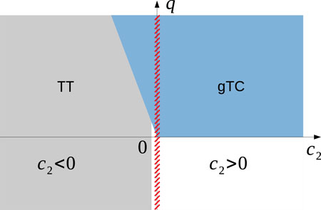
FIGURE 1. Time order phase diagram for spin-1 atomic BEC, where TT and gTC, respectively, denote time trivial and generalized time crystalline order. The region of (hashed) line segments surrounding c₂ = 0 for the non-interacting system is to be excluded.

More detailed discussions including the dependence of time order phases on system size, possible approaches to detect them, and extension to thermal state phases can be found in Section 4.

2.3 Time Order Phase Diagram for Quantum Rabi Model

As a second example, we consider time order phases of the quantum Rabi model described by the Hamiltonian as follows:

${\widehat{H}}_{\text{Rabi}}={\omega }_0{\widehat{a}}^{†}\widehat{a}+\frac{\mathrm{\Omega }}{2}{\widehat{\sigma }}_z-\lambda (\widehat{a}+{\widehat{a}}^{†}){\widehat{\sigma }}_x,(9)$

where ${\widehat{\sigma }}_{x,z}$ is the Pauli matrix of a two-level system (transition frequency Ω), $\widehat{a}({\widehat{a}}^{†})$ is the annihilation (creation) operator for a single bosonic field mode (of frequency ω₀), and λ is their coupling strength.

It is known that the aforementioned model exhibits a QPT to a superradiant state, despite its simplicity [29]. The transition occurs at the critical point g_c ≡ 1, with the dimensionless parameter $g\equiv 2\lambda /\sqrt{{\omega }_0\mathrm{\Omega }}$. The equivalent thermodynamic limit is approached by taking Ω/ω₀ → ∞. Though the system only has finite components, the QPT herein is well established. According to the studies in Ref. [29], an almost exact effective low-energy Hamiltonian for the normal phase (g < 1) is given by the following equation:

${\widehat{H}}_{\text{np}}={\omega }_0{\widehat{a}}^{†}\widehat{a}-\frac{{\omega }_0{g}^2}{4}{(\widehat{a}+{\widehat{a}}^{†})}^2-\frac{\mathrm{\Omega }}{2},(10)$

whose low-energy eigen-states are $|{\varphi }_{\text{np}}^m(g)\rangle =\widehat{\mathcal{S}}[r_{\text{np}}(g)]|m\rangle |\downarrow \rangle$ for g ≤ 1, with $\widehat{\mathcal{S}}[x]=\exp [x({\widehat{a}}^{†2}-{\widehat{a}}^2)/2]$ and r_np(g) = − [ln(1 − g²)]/4, and the energy eigen-values are $E_{\text{np}}^m(g)=m{ϵ}_{\text{np}}(g)+E_{\text{G,np}}(g)$, with ${ϵ}_{\text{np}}(g)={\omega }_0\sqrt{1-g^2}$ and E_G,np(g) = [ϵ_np(g) − ω₀]/2 − Ω/2. For the superradiant phase (g > 1), the effective low energy Hamiltonian becomes

${\widehat{H}}_{\text{sp}}={\omega }_0{\widehat{a}}^{†}\widehat{a}-\frac{{\omega }_0}{4g^4}{(\widehat{a}+{\widehat{a}}^{†})}^2-\frac{\mathrm{\Omega }}{4}(g^2+g^{-2}),(11)$

whose eigen-states are given by $|{\varphi }_{\text{sp}}^m{(g)\rangle }_{\pm }=\widehat{\mathcal{D}}[\pm {\alpha }_g]\widehat{\mathcal{S}}[r_{\text{sp}}(g)]|m\rangle |{\downarrow }^{\pm }\rangle$, with r_sp(g) = − [ln(1 − g⁻⁴)]/4, ${\alpha }_g=\sqrt{(\mathrm{\Omega }/4g^2{\omega }_0)(g^4-1)}$, and $\widehat{\mathcal{D}}[\alpha ]=e^{\alpha ({\widehat{a}}^{†}-\widehat{a})}$. The displacement-dependent spin states are $|{\downarrow }^{\pm }\rangle =\mp \sqrt{(1-g^{-2})/2}|\uparrow \rangle +\sqrt{(1+g^{-2})/2}|\downarrow \rangle$, while the energy eigen-values take the form $E_{\text{sp}}^m(g)=m{ϵ}_{\text{sp}}(g)+E_{\text{G,sp}}(g)$, with ${ϵ}_{\text{sp}}(g)={\omega }_0\sqrt{1-g^{-4}}$ and $E_{\mathrm{G},\mathrm{sp}}(g)=[{ϵ}_{\text{sp}}(g)-{\omega }_0]/2-\Omega (g^2+g^{-2})/4$. More details can be found in the supplementary material of Ref. [29].

For this model, the scaled average cavity photon number ${\widehat{n}}_c={\omega }_0{\widehat{a}}^{†}\widehat{a}/\mathrm{\Omega }$ is a suitable order parameter with Ω/ω₀ assuming the role of system size. The corresponding bulk order parameter then becomes ${\widehat{N}}_c={\widehat{a}}^{†}\widehat{a}$ or the average cavity photon number, and

$\begin{array}{cc}\hfill f(t)& ={\lim }_{\mathrm{\Omega }/{\omega }_0\to \infty }⟨{\widehat{n}}_c(t){\widehat{n}}_c(0)⟩,\hfill \\ \hfill F(t)& ={\lim }_{\mathrm{\Omega }/{\omega }_0\to \infty }⟨{\widehat{N}}_c(t){\widehat{N}}_c(0)⟩.\hfill \end{array}(12)$

For g < 1, we find

$\begin{array}{cc}\hfill f(t)& =0,\hfill \\ \hfill F(t)& ={\eta }_0+{\eta }_2{e}^{-i(2{ϵ}_{\text{np}})t},\hfill \end{array}(13)$

respectively, where η₀ =  sinh⁴(r_np) and η₂ =  cosh²(r_np) sinh²(r_np). For g > 1, we obtain the following equation:

$f(t)=\frac{{(g^2-g^{-2})}^2}{16}.(14)$

The time order phase diagram is shown in Figure 2. When g < 1, the system ground state corresponds to a generalized time crystalline order phase, while the system exhibits time trivial order when g > 1. Despites such a simple model composed of a two-level system and a bosonic field mode, the ground state of the quantum Rabi model displays an intriguing temporal phase structure accompanied by a finite-component quantum phase transition.

FIGURE 2

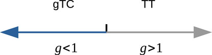
FIGURE 2. Time order phase diagram for the quantum Rabi model, where TT and gTC, respectively, denote time trivial and generalized time crystalline order.

2.4 Non-Hermitian Many-Body Interaction Model

Finally, we consider two effective models with many-body spin–spin interaction and non-Hermitian effects. The first is described by the Hamiltonian:

$\widehat{H}=-\frac{1}{N(N-1)}\sum _{1\le i<j\le N}(\lambda +\mathrm{i}\gamma ){\sigma }_1^x{\sigma }_2^x\cdots {\sigma }_{(i)}^y\cdots {\sigma }_{(j)}^y\cdots {\sigma }_N^x,(15)$

with two σ^y operators at sites i and j in a string of otherwise σ^x N-body spin interaction. 1/[N(N − 1)] is the normalization factor, λ is the spin interaction strength, and γ represents an effective dissipation rate. λ > 0 and γ ≥ 0 are both real numbers.

We observe that the Greenberger–Horne–Zeilinger (GHZ) states

$|G_{\pm }⟩=\frac{1}{\sqrt{2}}\left(|{0⟩}^{\otimes N}\pm |{1⟩}^{\otimes N}\right),(16)$

correspond to two non-degenerate system eigen-states with eigen-energies ± (λ + iγ)/2. The spectra of this model system are bounded inside the circle of radius $\sqrt{{\lambda }^2+{\gamma }^2}/2$ in the complex plane. The eigen-state whose eigen-value has the largest imaginary part is taken as the ground state, or |GS⟩ = |G₊⟩ with eigen-energy ϵ₀ = (λ + iγ)/2. The highest excited state is |G₋⟩, whose corresponding eigen-energy is ${ϵ}_{2^N-1}=-(\lambda +\mathrm{i}\gamma )/2$.

An appropriate order parameter operator in this case becomes the average magnetization $\widehat{m}={\sum }_{i=1}^N{\sigma }_i^z/N$. The twisted vector becomes $|v\rangle =\widehat{m}|\mathrm{G}\mathrm{S}\rangle =|G_{-}\rangle$, and the auto-correlator can be easily worked out to be $f(t)={\lim }_{N\to \infty }⟨\widehat{m}(t)\widehat{m}(0)⟩=e^{-i\lambda t}{e}^{\gamma t}$. When γ = 0, the system ground state exists time-crystalline order phase and corresponds to a continuous time crystal [33]. When γ ≠ 0, the system exhibits time functional order, with an exploding f(t) as time evolves.

A second non-Hermitian model Hamiltonian is given by

$\widehat{H}=(\lambda +\mathrm{i}\gamma )\left({\sigma }_1^x{\sigma }_2^x\cdots {\sigma }_{[N/2]}^x-{\sigma }_{[N/2]+1}^x\cdots {\sigma }_N^x\right)-\sum _{j=1}^N{\sigma }_j^z{\sigma }_{j+1}^z,(17)$

where [⋅] denotes the integer part, σ_N+1 ≡σ₁ corresponds to the periodic boundary condition, and λ and γ are spin-string interaction strength and dissipation strength, respectively, as in the previous model, and are real numbers. This Hamiltonian contains [(N + 1)/2]-body interaction terms and supports GHZ state |G₊⟩ as a non-degenerate excited state [18] with eigen-energy ϵ₊ = − N. The other two eigen-states of concern are $|{\mathrm{\Psi }}^{(\pm )}\rangle \equiv ({\alpha }_1|G_{-}\rangle +{\alpha }_2|{\tilde{G}}_{-,\mathcal{I}}\rangle )/\sqrt{|{\alpha }_1{|}^2+|{\alpha }_2{|}^2}$ with α₁ = 1 and α₂ = − (N + ϵ^(±))/2(λ + iγ), where

$|{\tilde{G}}_{-,\mathcal{I}}⟩=\frac{1}{\sqrt{2}}(|{0⟩}_1\cdots |{0⟩}_{[N/2]}|{1⟩}_{[N/2]+1}\cdots |{1⟩}_N-|{1⟩}_1\cdots |{1⟩}_{[N/2]}|{0⟩}_{[N/2]+1}\cdots |{0⟩}_N).(18)$

The eigen-energies for |Ψ^(±)⟩ are given by ${ϵ}^{(\pm )}=-N+2\pm 2\sqrt{1+{(\lambda +\mathrm{i}\gamma )}^2}$, with more details of the derivation given in Section 4. For the same order parameter operator $\widehat{m}$, we find $\widehat{m}|{\mathrm{\Psi }}_0\rangle \stackrel{N\to \infty }{\to }{\alpha }_1|G_{+}\rangle /\sqrt{|{\alpha }_1{|}^2+|{\alpha }_2{|}^2}$.

At γ = 0, the above non-Hermitian Hamiltonian Eq. 17 reduces to a Hermitian one, whose ground state |Ψ₀⟩ corresponds to the one with smaller ϵ from |Ψ⁽⁻⁾⟩ and |Ψ⁽⁺⁾⟩, or ${ϵ}_0=-N-2(\sqrt{1+{\lambda }^2}-1)$. The ground state |Ψ₀⟩ for this non-Hermitian system is therefore chosen from |Ψ⁽⁻⁾⟩ or |Ψ⁽⁺⁾⟩ to be the one that deforms into the right Hermitian case one when γ approaches zero. However, the criteria for the ground state energy ϵ₀ correspond to choosing the smaller one from ϵ^(±) when ϵ is real and choosing the one with the larger imaginary part when ϵ is complex.

Therefore, we directly obtain the following equation:

$f(t)={\lim }_{N\to \infty }⟨\widehat{m}(t)\widehat{m}(0)⟩=\frac{|{\alpha }_1{|}^2}{|{\alpha }_1{|}^2+|{\alpha }_2{|}^2}{e}^{-\mathrm{i}({ϵ}_{+}-{ϵ}_0)t}.(19)$

When λ ≠ 0 and γ ≠ 0, the system exists in time functional order phase and again results from the non-Hermitian Hamiltonian. When λ ≠ 0 but γ = 0, the auto-correlation function reduces to

$f(t)=\frac{1}{2}\left(1+\frac{1}{\sqrt{1+{\lambda }^2}}\right)e^{-2\mathrm{i}(\sqrt{1+{\lambda }^2}-1)t},(20)$

as for a genuine time crystal of the WO type exhibiting time crystalline order. When λ = 0 and 0 < |γ| ≤ 1, we find

$f(t)=\frac{1}{2}(1+\sqrt{1-{\gamma }^2})e^{-2\mathrm{i}(\sqrt{1-{\gamma }^2}-1)t}.(21)$

The system ground state again exhibits time-crystalline order. When λ = 0 and |γ| > 1, we obtain

$f(t)=\frac{1}{2}{e}^{2\mathrm{i}t}{e}^{-2\sqrt{{\gamma }^2-1}t},(22)$

by choosing ${ϵ}_0=-N+2+2\mathrm{i}\sqrt{{\gamma }^2-1}$ as the ground state eigen-energy from the two eigen-values $-N+2\pm 2\mathrm{i}\sqrt{{\gamma }^2-1}$. The system ground state now exhibits time functional order phase, with a decaying f(t) as time evolves. When λ = γ = 0,

$f(t)=1,(23)$

the ground state reduces to the time trivial order phase.

The above two non-Hermitian models represent direct generalizations of the Hermitian system as considered in Refs. [18, 33]. While slightly more complicated, they remain sufficiently simple for compact analytical treatment, thus helping to reveal interesting and clear physical meanings of the underlying time order.

2.5 Some Remarks About Continuous Time Crystal

According to the WO no-go theorem [62], f(t) for the ground state or the Gibbs ensemble of a general many-body Hamiltonian whose interactions are not-too-long ranged exhibits no temporal dependence; hence, it belongs to time trivial order according to our classification scheme. At first sight, this seems to sweep many important models of condensed matter physics into the same boring class of the time trivial order phase. However, it remains to explore, for instance, many-body systems with more than two-body (or k-body) interactions, or non-Hermitian systems, which might support the existence of CTC. Inspired by the recent results on CTC [33], we believe more time crystalline phases will be uncovered and further understanding will be gained in the future.

The two-time auto-correlation function f(t) measures the CTC phase as in earlier studies [33, 62], while both auto-correlation functions f(t) and F(t) together define different time-order phases we propose in this work. The absence of the local temporal behavior f(t) = 0 does not imply the absence of any temporal property in the bulk, when F(t) could have various temporal behaviors. Based on this, our operational definitions of time order are developed. We also extend the scope of CTC to include both TC order and gTC order phases. This distinction between f(t) and F(t) gives more insights into quantum many-body phases.

As emphasized earlier, continuous time crystal results from spontaneously breaking continuous time translation symmetry. Due to the genuine time periodicity contained in CTC, it might be possible to explore and design new types of clocks based on macroscopic many-body systems, as the time period is directly related to energy spectra, and whose physical meaning is clearly the same as for atomic clock states. Furthermore, they are not affected by finite size effect in contrast to periodicity in DTC.

3 Discussion and Conclusion

While ground-state phases of a quantum many-body system are mostly classified with their Hamiltonian based on the following two paradigms: LGW symmetry breaking order parameter or topological order, this work proposes to study phases from time dimension using time order or more specifically with the proposed symmetry-based time order. Compared to the recent progress and understanding gained for topological order [66, 67], one could try to develop a framework for entanglement-based time order instead of the symmetry-based time order we employ here in this study. Quantum entanglement in a many-body system is responsible for topological order, whose origin lies at the tensor product structure of the quantum many-body Hilbert space ${\mathcal{H}}_{\text{tot}}={\otimes }_i{\mathcal{H}}_i$ with ${\mathcal{H}}_i$ the finite-dimensional Hilbert space for site-i. An entanglement-based time order therefore calls for a combined investigation to exploit quantum entanglement and temporal properties of a quantum many-body system.

Through time order, one focuses on temporal structure of the evolution operator $e^{-i\widehat{H}t}$. The symmetry-based time order therefore unifies the LGW paradigm with the concept of time order, while an entanglement-based time order could amalgamate the topological order paradigm (or entanglement beyond that) with time order. For this to happen, a more basic definition for time order will be required, which will likely expand into further in-depth investigations.

In conclusion, understanding the phases of matter constitutes a cornerstone of contemporary physics. Capitalizing on the concept of CTC for the many-body ground state with perpetual time dependence, this study argues that information from time domain can be employed to classify the quantum phase as well, which provides a new perspective toward the understanding of ground-state time dependence, significantly beyond existing studies on CTC. We introduce time order, provide its operational definition in terms of two-time auto-correlation function of an appropriate symmetry order operator, bestow physical meaning to characteristic frequencies and amplitudes of the correlation function, and present a complete classification of time order phases. Time order phase diagrams for a spin-1 BEC system and the quantum Rabi model are fully worked out. Interesting time order phases in non-Hermitian spin models with multi-body interaction are presented. In addition to the time crystalline order which already attracts broad attention from its studies in terms of CTC, other phases we identify, for example, time quasi-crystalline order and time functional order, represent exciting new possibilities.

4 Methods and Calculation Details

Here, in this section, we provide more supporting material for our main results and related details for the aforementioned presentation. It is organized as follows: in Section 4.1, we extend the discussion of time order to finite temperature; in Section 4.2, we present calculation details related to the spin-1 atomic BEC example considered and give intriguing results for finite temperature scenario in spin-1 BEC; in Section 4.3,as a more straightforward approach to understand numerical results, we present a variational approach for treating the polar ground state of a spin-1 BEC. Finally, we give the details about ground state and eigen-energy calculation in the non-Hermitian quantum many-body model with multi-body interaction in Section 4.4.

4.1 Time Order at Finite Temperature

At finite temperature T, excited states will be populated, which can be taken into account with the Gibbs ensemble $\widehat{\rho }\equiv e^{-\beta \widehat{H}}/Z$, where $Z\equiv \text{Tr}{e}^{-\beta \widehat{H}}$ denotes the partition function and β ≡ 1/T the inverse temperature. We then find

$\begin{array}{ll}\hfill f(t)\to & {\lim }_{V\to \infty }\text{Tr}\left(e^{i\widehat{H}t}\widehat{\varphi }(0)e^{-i\widehat{H}t}\widehat{\varphi }(0)\widehat{\rho }\right)\hfill \\ \hfill =& {\lim }_{V\to \infty }\sum _{k=0}^{\infty }\langle {\psi }_k|e^{i\widehat{H}t}\widehat{\varphi }(0)e^{-i\widehat{H}t}\widehat{\varphi }(0)\frac{e^{-\beta \widehat{H}}}{Z}|{\psi }_k\rangle \hfill \\ \hfill =& {\lim }_{V\to \infty }\sum _{k=0}^{\infty }\frac{1}{Z}{e}^{i{ϵ}_{k}t-\beta {ϵ}_k}\langle v_k|e^{-i\widehat{H}t}|v_k\rangle \hfill \\ \hfill =& {\lim }_{V\to \infty }\sum _{k=0}^{\infty }\sum _{j=0}^{\infty }\frac{1}{Z}{c}_{jk}{e}^{-\beta {ϵ}_k}{e}^{-i({ϵ}_j-{ϵ}_k)t},\hfill \end{array}(24)$

where |v_k⟩ is the eigen-state twisted vector for |ψ_k⟩ and c_jk is its associated weight. Analogously, for the non-Hermitian case, we find

$\begin{array}{ll}\hfill f(t)=& {\lim }_{V\to \infty }\sum _{k=0}^{\infty }\frac{1}{Z}{e}^{i{ϵ}_{k}t-\beta {ϵ}_k}⟨v_k^{(l)}|e^{-i\widehat{H}t}|v_k^{(r)}⟩\hfill \\ \hfill =& {\lim }_{V\to \infty }\sum _{k=0}^{\infty }\sum _{j=0}^{\infty }\frac{1}{Z}{c}_{jk}{e}^{-\beta {ϵ}_k}{e}^{-i({ϵ}_j-{ϵ}_k)t},\hfill \end{array}(25)$

where $|v_k^{(l)}\rangle$ and $|v_k^{(r)}\rangle$ are the left and right twisted vectors for eigen-state |ψ_k⟩, respectively, and c_jk is the corresponding weight.

It is easily noted that f(t) at finite temperature contains contributions from all eigen-states of the quantum many-body system $\widehat{H}$, with a temperature-dependent weight factor for different energy levels, but f(t) remains to include contributions from different periodic functions. Hence, the quantum phase classification task essentially remains the same (including its possible reference to F(t)) as is shown in Table 1 for the ground state. At finite temperature, due to thermal excitations to the ground state, the temporal behavior will be more complex, thus opening up for more interesting possibilities, for example, to control time order phases and to study crossover or driven phase transitions between different time order phases.

4.2 Time Order in a Spin-1 Atomic BEC

For typical interaction parameters of a spin-1 BEC (e.g., of ground state ⁸⁷Rb or ²³Na atoms) in a tight trap, spin domain formation is energetically suppressed when the atom number is not too large as spin-dependent interaction strength is much weaker than spin-independent interaction [26, 32, 36, 58]. This facilitates a single-spatial-mode approximation (SMA) by assuming all spin states share the same spatial wave function ϕ(r), which effectively decouples the spatial degrees of freedom from the spin and results in the Hamiltonian [36, 44] in Eq. 6 for the model many-body system, where ${\widehat{a}}_{m_F}(m_F=0,\pm 1)$ is the annihilation operator of the ground manifold state |F = 1, m_F⟩ with corresponding number operator ${\widehat{N}}_{m_F}={\widehat{a}}_{m_F}^{†}{\widehat{a}}_{m_F}$. p and q are linear and quadratic Zeeman shifts which could be tuned independently in experiments [38], while c₂ denotes the spin exchange interaction strength. Unless otherwise noted, we will take |c₂| = 1 as unit of energy in this work. The total particle number operator $\widehat{N}={\widehat{N}}_1+{\widehat{N}}_0+{\widehat{N}}_{-1}$ and the longitudinal magnetization operator ${\widehat{F}}_z={\widehat{N}}_1-{\widehat{N}}_{-1}$ are both conserved. Thus, linear Zeeman shift can be set to p = 0 effectively.

As discussed in the main text, a suitable order parameter for this model system is ${\widehat{n}}_{\text{sum}}\equiv {\widehat{N}}_{\text{sum}}/N$ $({\widehat{N}}_{\text{sum}}={\widehat{N}}_1+{\widehat{N}}_{-1}=N-{\widehat{N}}_0)$, which measures the fractional atomic population in the states |1, 1⟩ and |1, − 1⟩, and N assumes the role of system size. Following our formulation and denoting the system energy eigen-state by |ψ_i⟩ (i = 0, 1, 2, ⋯) with increasing eigen-energy ϵ_i, the ground-state twisted vector becomes $|v\rangle \equiv {\widehat{n}}_{\text{sum}}|{\psi }_0\rangle ={\sum }_{i=0}^{\infty }{a}_i|{\psi }_i\rangle$, with a_i = ⟨ψ_i|v⟩ its expansion coefficient on the eigen-state |ψ_i⟩. We find

$f(t)={\lim }_{N\to \infty }⟨{\widehat{n}}_{\text{sum}}(t){\widehat{n}}_{\text{sum}}(0)⟩={\lim }_{N\to \infty }\sum _{j=0}^{\infty }{b}_j{e}^{-i({ϵ}_j-{ϵ}_0)t},(26)$

where b_j ≡|a_j|² is the weight of the ground-state twisted vector, $b\equiv {\sum }_{j=0}^{\infty }{b}_j$ the total weight, and

$F(t)={\lim }_{N\to \infty }⟨{\widehat{N}}_{\text{sum}}(t){\widehat{N}}_{\text{sum}}(0)⟩={\lim }_{N\to \infty }\sum _{j=0}^{\infty }{B}_j{e}^{-i({ϵ}_j-{ϵ}_0)t},(27)$

where A_i = N⟨ψ_i|v⟩, B_j ≡|A_j|² is the weight of the enlarged ground state twisted vector, and $B\equiv {\sum }_{j=0}^{\infty }{B}_j$ the total weight.

Our study below is for the zero magnetization F_z = 0 subspace and employs exact diagonalization (ED) to calculate eigen-states as well as eigen-energies. The overall time order phase diagram for spin-1 BEC is shown in Figure 1. For ferromagnetic interaction c₂ < 0, the critical quadratic Zeeman energy q/|c₂| = 2 splits the whole region into the time trivial order (TT) phase for smaller q that observes TTS, and the generalized time crystalline (gTC) order phase for q/|c₂| > 2 where TTS is spontaneously broken. The latter (gTC phase) is found to coincide with the ground-state polar phase. The available computation resource limits the calculation to a finite system size, which prevents us from mapping out the exact details in the immediate neighborhood of q = 2, where further elaboration is needed for its time order properties. On the other hand, for antiferromagnetic interactions, we find q = 0 separates TT phase from gTC order.

In Figure 3, the weights for the ground state as well as for the low-lying excited states are shown as functions of q for a typical system size of N = 10 000. Only the ground-state weight b₀ is non-vanishing in the q < 2 (q < 0) region for ferromagnetic (antiferromagnetic) interactions, but total weight b is zero in the q > 2 (q > 0) region for ferromagnetic (antiferromagnetic) interaction, which prompts us to examine further the enlarged weights B_i corresponding to the bulk order parameter. For ground and the first excited states, the volume enlarged weights B_0,1 are found to be non-vanishing, although both decrease as q increases and grow with N as q approaches q = 2 (q = 0) for ferromagnetic (antiferromagnetic) interaction. However, as mentioned above, limited to a system size of N = 10 000 by computation resource in the ED calculation, we cannot exactly map out the behavior near q = 2 (q = 0) for ferromagnetic (antiferromagnetic) interaction. This consequently leaves empty for q in region [2.0, 2.02] ([0, 0.01]) for ferromagnetic (antiferromagnetic) interaction.

FIGURE 3

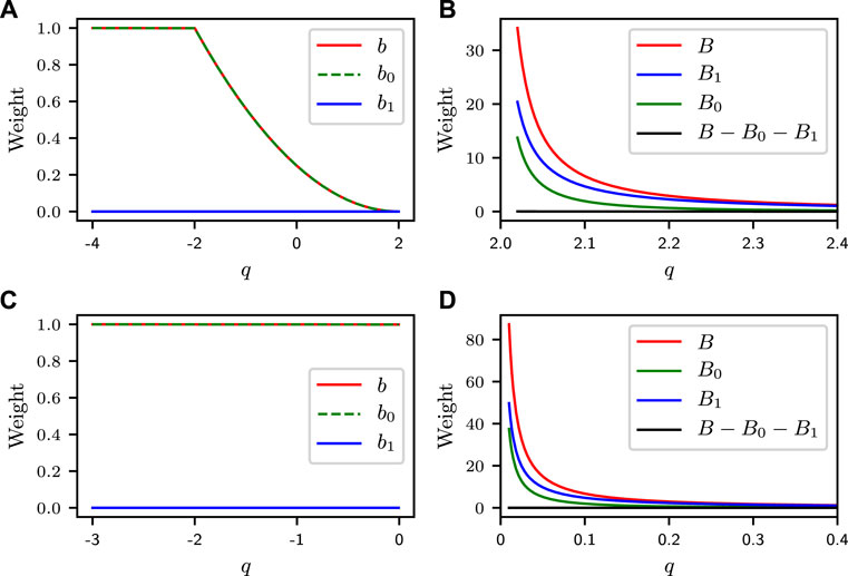
FIGURE 3. Weights of ground-state twisted vector in the ground and low-lying excited states as functions of q at system size N = 10 000. The upper panel is for ferromagnetic interaction, where weights b_i for q < 2 are shown in (A), while weights B_i for q > 2 are shown in (B). The lower panel is for antiferromagnetic interaction, where weights b_i for q < 0 are shown in (C), while weights B_i for q > 0 are shown in (D).

The dependence on system size N is clearly revealed by Figure 4, with the enlarged weights in the gTC regime attaining fixed values as the system approaches thermodynamic limit (N → ∞). In regions away from q = 2 (q = 0) for ferromagnetic (antiferromagnetic) interaction, ED numerics can always approach thermodynamic limit, except for the immediate neighborhood near q = 2 (q = 0), where we infer with confidence the tendencies to divergence of the weights B_0,1 as q approaches q = 2 (q = 0).

FIGURE 4

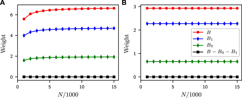
FIGURE 4. Weights of ground-state twisted vector in the ground and low-lying excited states as functions of system size N at q = 2.1 for ferromagnetic interaction (A) and at q = 0.2 for antiferromagnetic interaction (B).

The time evolution of two-time auto-correlation function F(t) is plotted in Figures 5A,C for ferromagnetic and for antiferromagnetic interactions, while Figures 5B,D display energy gaps between ground and the first excited states as a function of q for ferromagnetic and antiferromagnetic interactions, respectively, at a system size of N = 5000. The behavior of F(t) is quantitatively consistent with that of the weights B_i(q) (i = 0, 1) shown in Figure 3 and the energy gap ϵ₁ − ϵ₀ shown in Figures 5B,D.

FIGURE 5

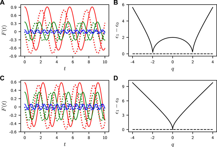
FIGURE 5. F(t) for different q as a function of time t. The solid and dotted lines correspond to Re(F) and Im(F), respectively. The red, green, and blue lines correspond to q = 2.5, q = 3, and q = 5, respectively, for ferromagnetic interaction (A). The red, green, and blue lines correspond to q = 0.7, q = 1, and q = 3, respectively for antiferromagnetic interaction (C). The energy gap between ground and the first excited state ϵ₁ − ϵ₀ as a function of q for ferromagnetic (B) and antiferromagnetic interactions (D), at system size N = 5000.

At finite temperature, excited states come into play by also contributing to the correlation function. We find the gTC order hosted in the polar phase persists for both ferromagnetic and antiferromagnetic interactions. The corresponding time evolution and Fourier transform of F(t) are shown in Figure 6, calculated for N = 500 at a temperature of β ≡ 1/T = 1. The Fourier transform is performed for Re(F) over t = [0, 1000] with the zero frequency (DC) component subtracted or for Im(F). The upper (lower) panel corresponds to ferromagnetic (antiferromagnetic) interaction at q = 3 (q = 2). For ferromagnetic interaction, two distinct frequency components are clearly identified for q = 3, associated with the two different energy level gaps. The beautiful beat pattern for F(t) would appear, while we only show the short time behavior in Figure 6 (a). Thus, the gTC phase remains at a finite temperature. Moreover, we also find a generalized time quasi-crystalline order phase assuming the two frequencies are incommensurate, by fine-tuning their corresponding energy gaps such that the relation Δ₁/Δ₂ = m₁/m₂ with m₁ and m₂ being co-primes is not satisfied. The gTC phase at finite temperature here is robust which is in contrast to the melting behavior of continuous time crystal (CTC) shown in Ref. [33].

FIGURE 6

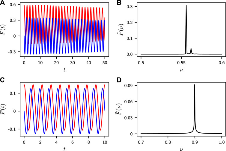
FIGURE 6. F(t) as a function of time t at q = 3 for ferromagnetic interaction (A) and q = 2 for antiferromagnetic interaction (C). The red and blue solid lines, respectively, correspond to Re(F) and Im(F). The Fourier transform spectrum $\tilde{F}(\nu )$ of Re(F) or Im(F) with ν = 1/T the frequency, T the period, for ferromagnetic (B) and antiferromagnetic (D) interactions, at temperature β = 1 and system size N = 500.

Finally, we hope to address the critical question about how could this time order, sort of a perpetual time dependence, can be observed. We note the bulk two-time auto-correlation function introduced $F(t)={\lim }_{N\to \infty }⟨{\widehat{N}}_{\text{sum}}(t){\widehat{N}}_{\text{sum}}(0)⟩$ denotes nothing but the ground-state (averaged) conditional outcome of measuring N_sum(t) at t after starting with N_sum(0) initially. The dynamics of F(t) follows that of N_sum(t) as in the quantum regression theorem. Given the system is well controlled, highly reproducible, one can simply detect F(t) by measuring N_sum(t), although for each measurement at an instant t, a condensate is destroyed, and a follow-up one will have to be prepared as closely as possible in every respects (through selection and post-selection) and be measured at a different t′ > t. Thus, a plausible way to detect the ground-state time dependence will require reconstructing the time dependence of F(t)/N_sum(0). As long as the oscillation amplitude is more than a few percent, it will be easily observable with not too much difficulty, although such a reconstruction will still be difficult as N_sum(0) can be rather small compared to N₀ ∼ N in the polar state. Alternatively, one can perhaps start from a twin-Fock state, that is, by preparing an initial state with N_sum(0) ∼ N.

In Figure 7A, we show the behavior of oscillation amplitude for F(t)/N_sum(0). The time dependence of F(t)/N_sum(0) at q = 2.5 for ferromagnetic interaction is shown in Figure 7B.

FIGURE 7

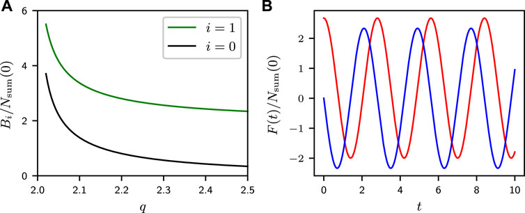
FIGURE 7. (A) B_i/N_sum(0) as a function of q for ferromagnetic interaction. (B) F(t)/N_sum(0) as a function of time t at q = 2.5 for ferromagnetic interaction. The red and blue solid lines correspond to the real and imaginary part of F(t)/N_sum(0), respectively.

4.3 A Variational Polar State for Ferromagnetic Spin-1 BEC

One might naively expect that nothing particularly interesting could happen in the polar phase of a ferromagnetic spin-1 BEC, where essentially all atoms reside in the single particle state |1, 0⟩. Nevertheless, due to the competition between spin exchange interaction c₂ and quadratic Zeeman shift q, the ground state of our system differs from |N₁ = 0, N₀ = N, N₋₁ = 0⟩, which can be affirmed based on a simple variational analytical calculation given in this section.

We use the number-state basis |N₁, N₀, N₋₁⟩ ≡|[N], M, k⟩, where $N_{m_F}$ denotes the occupation number of the m_F magnetic state, M ≡ N₁ − N₋₁, and k ≡ N₋₁. We take the following ground-state variational ansatz $|{\psi }_0\rangle =\frac{1}{\sqrt{1+|a{|}^2}}\left(|0,N,0\rangle +a|1,N-\mathrm{2,1}\rangle \right)$ for the polar state of ferromagnetic spin-1 BEC, where a = re^iϕ is a (complex) variational parameter with r and ϕ as real parameters. From Eq. 6 and (assumed) p = 0, the ground-state energy follows from

$\begin{array}{ll}\hfill E=& \frac{\langle {\psi }_0|H|{\psi }_0\rangle }{\langle {\psi }_0|{\psi }_0\rangle }\hfill \\ \hfill =& \frac{1}{1+a\ast a}\left[\left(\frac{c_2(2N-5)}{N}+2q\right)a\ast a+c_2\sqrt{\frac{N-1}{N}}(a\ast +a)\right]\hfill \\ \hfill =& \frac{1}{1+r^2}\left[\left(\frac{c_2(2N-5)}{N}+2q\right)r^2+2c_2\sqrt{\frac{N-1}{N}}r\cos (\varphi )\right].\hfill \end{array}(28)$

We see the extreme value (the minimum) of E is reached when cos(ϕ) = ±1, that is, for a real variational parameter a, which will be assumed from now on. This gives the following equation:

$E=\frac{x_1{a}^2+x_{2}a}{1+a^2},(29)$

with $x_1=\frac{c_2(2N-5)}{N}+2q$ and $x_2=2c_2\sqrt{\frac{N-1}{N}}$. The derivative of the energy function E(a) is as follows:

$E^{\prime }(a)=\frac{-x_2{a}^2+2x_{1}a+x_2}{{(1+a^2)}^2},(30)$

which determines the locations for the extreme values.

$a_{\pm }=\frac{1}{2c_2\sqrt{N(N-1)}}\left[c_2(2N-5)+2Nq\pm N\sqrt{\frac{c_2^2(8N^2-24N+25)}{N^2}+\frac{4c_{2}q(2N-5)}{N}+4q^2}\right],(31)$

and the corresponding extreme values are as follows:

$E_{\pm }=c_2+q\pm \frac{1}{2}\sqrt{4q^2+8c_{2}q+8c_2^2+\frac{-24c_2^2-10c_{2}q}{N}+\frac{25c_2^2}{N^2}}-\frac{5c_2}{2N}.(32)$

In the thermodynamic limit N → ∞, they reduce, respectively, to $a_{\pm }=1+\frac{q}{c_2}\pm \frac{\sqrt{2c_2^2+2c_{2}q+q^2}}{c_2}$ and $E_{\pm }=c_2+q\pm \sqrt{2c_2^2+2c_{2}q+q^2}$. The left and right asymptotic value for the energy function E(a) is therefore

$E(a)=c_2\left(2-\frac{5}{N}\right)+2q,(\text{when}a\to \pm \infty ).(33)$

For ferromagnetic interaction (c₂ < 0), E₋ assumes the minimum, which corresponds to the ground state $|{\psi }_0\rangle =\frac{1}{\sqrt{1+a_{-}^2}}\left(|0,N,0\rangle +a_{-}|1,N-\mathrm{2,1}\rangle \right)$ with $N_{\text{sum}}=2a_{-}^2/(1+a_{-}^2)$, and $a_{-}=1+\frac{q}{c_2}-\frac{\sqrt{2c_2^2+2c_{2}q+q^2}}{c_2}$ in the thermodynamic limit N → ∞.

Despite the vanishing order parameter n_sum in the polar phase (here the gTC order phase from the time order perspective), the enlarged quantity N_sum retains a finite value. Hence, the physics we present here clearly belongs to the realm of quantum effects, beyond the reach of mean-field theory.

4.4 The Non-Hermitian Spin Model With Multi-Body Interaction

The non-Hermitian quantum many-body model Hamiltonian is

$\widehat{H}={\widehat{H}}_0+(\lambda +\gamma \mathrm{i}){\widehat{H}}_1,(34)$

with

$\begin{array}{cc}\hfill {\widehat{H}}_0& =-\sum _{j=1}^N{\sigma }_j^z{\sigma }_{j+1}^z,\hfill \\ \hfill {\widehat{H}}_1& ={\sigma }_1^x{\sigma }_2^x\cdots {\sigma }_{[N/2]}^x-{\sigma }_{[N/2]+1}^x\cdots {\sigma }_N^x,\hfill \end{array}(35)$

where [⋅] denotes the integral part, σ_N+1 ≡σ₁, λ, and γ are spin-string interaction strength and dissipation strength, respectively. λ and γ are both real numbers. i is the imaginary unit. σ^x,y,z are Pauli operators. N is the qubit number of the system. The Hamiltonian has the [(N + 1)/2]-body interaction term and supports the GHZ state |G₊⟩ as a non-degenerate excited state.

First, the Greenberger–Horne–Zeilinger (GHZ) states are denoted as follows:

$|G_{\pm }⟩=\frac{1}{2}(|{0⟩}^{\otimes N}\pm |{1⟩}^{\otimes N}),(36)$

and

$|{\tilde{G}}_{-,\mathcal{I}}⟩=\frac{1}{\sqrt{2}}\left(|{0⟩}_1\cdots |{0⟩}_{[N/2]}|{1⟩}_{[N/2]+1}\cdots |{1⟩}_N-|{1⟩}_1\cdots |{1⟩}_{[N/2]}|{0⟩}_{[N/2]+1}\cdots |{0⟩}_N\right),(37)$

where $\mathcal{I}=([N/2]+1,[N/2]+2,\dots ,N)$ is a multi-index.

We immediately know that |G_±⟩ is the degenerate ground state of the ferromagnetic Ising Hamiltonian ${\widehat{H}}_0$ with eigen-energy E₍₀₎ = − N, $|{\tilde{G}}_{-,\mathcal{I}}\rangle$ is the excited state of ${\widehat{H}}_0$ with eigen-energy E₍₁₎ = − N + 4.

The action of $\widehat{H_1}$ on |G₋⟩ $(|{\tilde{G}}_{-,\mathcal{I}}\rangle )$ gives $|{\tilde{G}}_{-,\mathcal{I}}\rangle$ (|G₋⟩) with a multiplicative factor –2.

$\begin{array}{cc}\hfill {\widehat{H}}_1|G_{-}\rangle & =-2|{\tilde{G}}_{-,\mathcal{I}}\rangle ,\hfill \\ \hfill {\widehat{H}}_1|{\tilde{G}}_{-,\mathcal{I}}\rangle & =-2|G_{-}\rangle .\hfill \end{array}(38)$

Then we know the two eigen-states of $\widehat{H}$ are a superposition of |G₋⟩ and $|{\tilde{G}}_{-,\mathcal{I}}\rangle$, and can be written as

$|\mathrm{\Psi }⟩={\alpha }_1|G_{-}⟩+{\alpha }_2|{\tilde{G}}_{-,\mathcal{I}}⟩,(39)$

where α_1,2 are the undetermined coefficients. By substituting into the Schrödinger equation $\widehat{H}\mathrm{\Psi }\rangle =ϵ|\mathrm{\Psi }\rangle$, we get

$\begin{array}{ll}\hfill {ϵ}^2-\left(E_{(0)}+E_{(1)}\right)ϵ+\left(E_{(0)}{E}_{(1)}-4{(\lambda +\gamma \mathrm{i})}^2\right)& =0,\hfill \end{array}(40)$

$\begin{array}{ll}\hfill 2(\lambda +\gamma \mathrm{i}){\alpha }_2& =(E_{(0)}-ϵ){\alpha }_1.\hfill \end{array}(41)$

We obtain the eigen-energy ${ϵ}^{(\pm )}=\frac{1}{2}[E_{(0)}+E_{(1)}\pm \sqrt{{(E_{(1)}-E_{(0)})}^2+16{(\lambda +\gamma \mathrm{i})}^2}]$. Choosing ${\alpha }_1=1$, we have ${\alpha }_2=\frac{E_{(0)}-ϵ}{2(\lambda +\gamma \mathrm{i})}$. Imposing the normalization condition, we have the following equation:

$|{\mathrm{\Psi }}^{(\pm )}⟩=\frac{{\alpha }_1}{\sqrt{|{\alpha }_1{|}^2+|{\alpha }_2{|}^2}}|G_{-}⟩+\frac{{\alpha }_2}{\sqrt{|{\alpha }_1{|}^2+|{\alpha }_2{|}^2}}|{\tilde{G}}_{-,\mathcal{I}}⟩.(42)$

If γ = 0, the Hamiltonian is Hermitian, and we have the ground state |Ψ₀⟩ ≡|Ψ⁽⁻⁾⟩ with energy ${ϵ}_0\equiv {ϵ}^{(-)}=-N-2(\sqrt{1+{\lambda }^2}-1)$ (see more details about the Hermitian version of the system in Ref. [18]). Here, we choose the eigen-state from {|Ψ⁽⁺⁾⟩, |Ψ⁽⁻⁾⟩} as the ground state |Ψ₀⟩ of our generalized non-Hermitian system, for it deforms into the ground state of the Hermitian case when γ approaches zero. If ϵ is real, then ground-state energy ϵ₀ corresponds to the smaller one from ϵ^(±). However, ground-state energy ϵ₀ corresponds to the one with the larger imaginary part when ϵ is a complex number. Ground state |Ψ₀⟩ is obtained straightforwardly.

For the GHZ state |G₊⟩, we can know it is a non-degenerate excited state with energy ϵ₊ = − N, for

${\widehat{H}}_1|G_{+}⟩=0.(43)$

Data Availability Statement

The raw data supporting the conclusions of this article will be made available by the authors, without undue reservation.

Author Contributions

T-CG proposed and conducted the research, LY supervised the research, and T-CG, LY discussed the results and wrote the manuscript.

Funding

This work is supported by the National Key R&D Program of China (grant no. 2018YFA0306504), the National Natural Science Foundation of China (NSFC) (grants nos. 11 654001 and U1930201), and the Key-Area Research and Development Program of GuangDong Province (grant no. 2019B030330001).

Conflict of Interest

The authors declare that the research was conducted in the absence of any commercial or financial relationships that could be construed as a potential conflict of interest.

Publisher’s Note

All claims expressed in this article are solely those of the authors and do not necessarily represent those of their affiliated organizations, or those of the publisher, the editors, and the reviewers. Any product that may be evaluated in this article, or claim that may be made by its manufacturer, is not guaranteed or endorsed by the publisher.

Acknowledgments

T-CG thanks Qi Liu and Ming Xue for their helpful discussion about spinor Bose–Einstein condensate.

References

1. Anquez M, Robbins BA, Bharath HM, Boguslawski M, Hoang TM, Chapman MS Quantum Kibble-Zurek Mechanism in a Spin-1 Bose-Einstein Condensate. Phys Rev Lett (2016) 116:155301. doi:10.1103/physrevlett.116.155301

PubMed Abstract | CrossRef Full Text | Google Scholar

2. Autti S, Eltsov VB, Volovik GE Observation of a Time Quasicrystal and its Transition to a Superfluid Time crystal. Phys Rev Lett (2018) 120:215301. doi:10.1103/PhysRevLett.120.215301

PubMed Abstract | CrossRef Full Text | Google Scholar

3. Bruno P Impossibility of Spontaneously Rotating Time Crystals: A No-Go Theorem. Phys Rev Lett (2013) 111:070402. doi:10.1103/PhysRevLett.111.070402

PubMed Abstract | CrossRef Full Text | Google Scholar

4. Buča B, Tindall J, Jaksch D Non-stationary Coherent Quantum many-body Dynamics through Dissipation. Nat Commun (2019) 10:1730. doi:10.1038/s41467-019-09757-y

PubMed Abstract | CrossRef Full Text | Google Scholar

5. Buča B, Jaksch D Dissipation Induced Nonstationarity in a Quantum Gas. Phys Rev Lett (2019) 123:260401. doi:10.1103/PhysRevLett.123.260401

PubMed Abstract | CrossRef Full Text | Google Scholar

6. Cai Z, Huang Y, Vincent Liu W Imaginary Time crystal of thermal Quantum Matter. Chin Phys. Lett. (2020) 37:050503. doi:10.1088/0256-307x/37/5/050503

CrossRef Full Text | Google Scholar

7. Chang M-S, Hamley CD, Barrett MD, Sauer JA, Fortier KM, Zhang W, et al. Observation of Spinor Dynamics in Optically TrappedRb87Bose-Einstein Condensates. Phys Rev Lett (2004) 92:140403. doi:10.1103/physrevlett.92.140403

PubMed Abstract | CrossRef Full Text | Google Scholar

8. Chang M-S, Qin Q, Zhang W, You L, Chapman MS Coherent Spinor Dynamics in a Spin-1 Bose Condensate. Nat Phys (2005) 1:111–6. doi:10.1038/nphys153

CrossRef Full Text | Google Scholar

9. Chen X, Burnell FJ, Vishwanath A, Fidkowski L Anomalous Symmetry Fractionalization and Surface Topological Order. Phys Rev X (2015) 5:041013. doi:10.1103/PhysRevX.5.041013

CrossRef Full Text | Google Scholar

10. Chen X, Gu Z-C, Liu Z-X, Wen X-G Symmetry Protected Topological Orders and the Group Cohomology of Their Symmetry Group. Phys Rev B (2013) 87:155114. doi:10.1103/PhysRevB.87.155114

CrossRef Full Text | Google Scholar

11. Chen X, Liu Z-X, Wen X-G Two-dimensional Symmetry-Protected Topological Orders and Their Protected Gapless Edge Excitations. Phys Rev B (2011) 84:235141. doi:10.1103/PhysRevB.84.235141

CrossRef Full Text | Google Scholar

12. Cheng M, Gu Z-C, Jiang S, Qi Y Exactly Solvable Models for Symmetry-Enriched Topological Phases. Phys Rev B (2017) 96:115107. doi:10.1103/PhysRevB.96.115107

CrossRef Full Text | Google Scholar

13. Choi S, Choi J, Landig R, Kucsko G, Zhou H, Isoya J, et al. Observation of Discrete Time-Crystalline Order in a Disordered Dipolar many-body System. Nature (2017) 543:221–5. doi:10.1038/nature21426

PubMed Abstract | CrossRef Full Text | Google Scholar

14. Cosme JG, Skulte J, Mathey L Time Crystals in a Shaken Atom-Cavity System. Phys Rev A (2019) 100:053615. doi:10.1103/PhysRevA.100.053615

CrossRef Full Text | Google Scholar

15. Damski B, Zurek WH Dynamics of a Quantum Phase Transition in a Ferromagnetic Bose-Einstein Condensate. Phys Rev Lett (2007) 99:130402. doi:10.1103/PhysRevLett.99.130402

PubMed Abstract | CrossRef Full Text | Google Scholar

16. Else DV, Bauer B, Nayak C. Floquet Time Crystals. Phys Rev Lett (2016) 117:090402. doi:10.1103/PhysRevLett.117.090402

PubMed Abstract | CrossRef Full Text | Google Scholar

17. Else DV, Monroe C, Nayak C, Yao NY Discrete Time Crystals. Annu Rev Condens Matter Phys (2020) 11:467–99. doi:10.1146/annurev-conmatphys-031119-050658

CrossRef Full Text | Google Scholar

18. Facchi P, Florio G, Pascazio S, Pepe FV Greenberger-horne-zeilinger States and Few-Body Hamiltonians. Phys Rev Lett (2011) 107:260502. doi:10.1103/PhysRevLett.107.260502

PubMed Abstract | CrossRef Full Text | Google Scholar

19. Fan C-h., Rossini D, Zhang H-X, Wu J-H, Artoni M, La Rocca GC Discrete Time crystal in a Finite Chain of Rydberg Atoms without Disorder. Phys Rev A (2020) 101:013417. doi:10.1103/PhysRevA.101.013417

CrossRef Full Text | Google Scholar

20. Fradkin E Field Theories of Condensed Matter Physics. 2nd ed. Oxford, UK: Oxford University Press (2004).

Google Scholar

21. Gambetta FM, Carollo F, Marcuzzi M, Garrahan JP, Lesanovsky I Discrete Time Crystals in the Absence of Manifest Symmetries or Disorder in Open Quantum Systems. Phys Rev Lett (2019) 122:015701. doi:10.1103/PhysRevLett.122.015701

PubMed Abstract | CrossRef Full Text | Google Scholar

22. Gong Z, Hamazaki R, Ueda M Discrete Time-Crystalline Order in Cavity and Circuit Qed Systems. Phys Rev Lett (2018) 120:040404. doi:10.1103/PhysRevLett.120.040404

PubMed Abstract | CrossRef Full Text | Google Scholar

23. Gu Z-C, Wen X-G Tensor-entanglement-filtering Renormalization Approach and Symmetry-Protected Topological Order. Phys Rev B (2009) 80:155131. doi:10.1103/PhysRevB.80.155131

CrossRef Full Text | Google Scholar

24. Guzman J, Jo G-B, Wenz AN, Murch KW, Thomas CK, Stamper-Kurn DM Long-time-scale Dynamics of Spin Textures in a Degenerate F = 1⁸⁷rb Spinor Bose Gas. Phys Rev A (2011) 84:063625. doi:10.1103/physreva.84.063625

CrossRef Full Text | Google Scholar

25. Heinrich C, Burnell F, Fidkowski L, Levin M Symmetry-enriched String Nets: Exactly Solvable Models for Set Phases. Phys Rev B (2016) 94:235136. doi:10.1103/PhysRevB.94.235136

CrossRef Full Text | Google Scholar

26. Ho T-L Spinor Bose Condensates in Optical Traps. Phys Rev Lett (1998) 81:742–5. doi:10.1103/PhysRevLett.81.742

CrossRef Full Text | Google Scholar

27. Huang B, Wu Y-H, Liu WV Clean Floquet Time Crystals: Models and Realizations in Cold Atoms. Phys Rev Lett (2018) 120:110603. doi:10.1103/PhysRevLett.120.110603

PubMed Abstract | CrossRef Full Text | Google Scholar

28. Hurtado-Gutiérrez R, Carollo F, Pérez-Espigares C, Hurtado PI Building Continuous Time Crystals from Rare Events. Phys Rev Lett (2020) 125:160601. doi:10.1103/PhysRevLett.125.160601

PubMed Abstract | CrossRef Full Text | Google Scholar

29. Hwang M-J, Puebla R, Plenio MB Quantum Phase Transition and Universal Dynamics in the Rabi Model. Phys Rev Lett (2015) 115:180404. doi:10.1103/PhysRevLett.115.180404

PubMed Abstract | CrossRef Full Text | Google Scholar

30. Iemini F, Russomanno A, Keeling J, Schirò M, Dalmonte M, Fazio R Boundary Time Crystals. Phys Rev Lett (2018) 121:035301. doi:10.1103/PhysRevLett.121.035301

PubMed Abstract | CrossRef Full Text | Google Scholar

31. Khemani V, Lazarides A, Moessner R, Sondhi SL Phase Structure of Driven Quantum Systems. Phys Rev Lett (2016) 116:250401. doi:10.1103/PhysRevLett.116.250401

PubMed Abstract | CrossRef Full Text | Google Scholar

32. Koashi M, Ueda M Exact Eigenstates and Magnetic Response of Spin-1 and Spin-2 Bose-Einstein Condensates. Phys Rev Lett (2000) 84:1066–9. doi:10.1103/PhysRevLett.84.1066

PubMed Abstract | CrossRef Full Text | Google Scholar

33. Kozin VK, Kyriienko O Quantum Time Crystals from Hamiltonians with Long-Range Interactions. Phys Rev Lett (2019) 123:210602. doi:10.1103/PhysRevLett.123.210602

PubMed Abstract | CrossRef Full Text | Google Scholar

34. Lamacraft A Quantum Quenches in a Spinor Condensate. Phys Rev Lett (2007) 98:160404. doi:10.1103/physrevlett.98.160404

PubMed Abstract | CrossRef Full Text | Google Scholar

35. Landau LD, Lifshitz E Statistical Physics. Oxford, UK: Butterworth-Heinemann (1999).

Google Scholar

36. Law CK, Pu H, Bigelow NP Quantum Spins Mixing in Spinor Bose-Einstein Condensates. Phys Rev Lett (1998) 81:5257–61. doi:10.1103/PhysRevLett.81.5257

CrossRef Full Text | Google Scholar

37. Lazarides A, Roy S, Piazza F, Moessner R Time Crystallinity in Dissipative Floquet Systems. Phys Rev Res (2020) 2:022002. doi:10.1103/PhysRevResearch.2.022002

CrossRef Full Text | Google Scholar

38. Luo XY, Zou YQ, Wu LN, Liu Q, Han MF, Tey MK, et al. Deterministic Entanglement Generation from Driving through Quantum Phase Transitions. Science (2017) 355:620–3. doi:10.1126/science.aag1106

PubMed Abstract | CrossRef Full Text | Google Scholar

39. Machado F, Else DV, Kahanamoku-Meyer GD, Nayak C, Yao NY Long-range Prethermal Phases of Nonequilibrium Matter. Phys Rev X (2020) 10:011043. doi:10.1103/PhysRevX.10.011043

CrossRef Full Text | Google Scholar

40. Medenjak M, Buča B, Jaksch D Isolated Heisenberg Magnet as a Quantum Time crystal. Phys Rev B (2020) 102:041117. doi:10.1103/PhysRevB.102.041117

CrossRef Full Text | Google Scholar

41. Mierzejewski M, Giergiel K, Sacha K Many-body Localization Caused by Temporal Disorder. Phys Rev B (2017) 96:140201. doi:10.1103/PhysRevB.96.140201

CrossRef Full Text | Google Scholar

42. Nozières P Time Crystals: Can Diamagnetic Currents Drive a Charge Density Wave into Rotation? Europhysics Lett (2013) 103:57008. doi:10.1209/0295-5075/103/57008

CrossRef Full Text | Google Scholar

43. Pal S, Nishad N, Mahesh TS, Sreejith GJ Temporal Order in Periodically Driven Spins in star-shaped Clusters. Phys Rev Lett (2018) 120:180602. doi:10.1103/PhysRevLett.120.180602

PubMed Abstract | CrossRef Full Text | Google Scholar

44. Pu H, Law CK, Raghavan S, Eberly JH, Bigelow NP Spin-mixing Dynamics of a Spinor Bose-Einstein Condensate. Phys Rev A (1999) 60:1463–70. doi:10.1103/PhysRevA.60.1463

CrossRef Full Text | Google Scholar

45. Qiu LY, Liang HY, Yang YB, Yang HX, Tian T, Xu Y, et al. Observation of Generalized Kibble-Zurek Mechanism across a First-Order Quantum Phase Transition in a Spinor Condensate. Sci Adv (2020) 6:eaba7292. doi:10.1126/sciadv.aba7292

PubMed Abstract | CrossRef Full Text | Google Scholar

46. Riera-Campeny A, Moreno-Cardoner M, Sanpera A Time Crystallinity in Open Quantum Systems. Quantum (2020) 4:270. doi:10.22331/q-2020-05-25-270

CrossRef Full Text | Google Scholar

47. Rovny J, Blum RL, Barrett SE P31 NMR Study of Discrete Time-Crystalline Signatures in an Ordered crystal of Ammonium Dihydrogen Phosphate. Phys Rev B (2018) 97:184301. doi:10.1103/PhysRevB.97.184301

CrossRef Full Text | Google Scholar

48. Rovny J, Blum RL, Barrett SE Observation of Discrete-Time-crystal Signatures in an Ordered Dipolar many-body System. Phys Rev Lett (2018) 120:180603. doi:10.1103/PhysRevLett.120.180603

PubMed Abstract | CrossRef Full Text | Google Scholar

49. Russomanno A, Iemini F, Dalmonte M, Fazio R Floquet Time crystal in the Lipkin-Meshkov-Glick Model. Phys Rev B (2017) 95:214307. doi:10.1103/PhysRevB.95.214307

CrossRef Full Text | Google Scholar

50. Sacha K Anderson Localization and mott Insulator Phase in the Time Domain. Sci Rep (2015) 5:10787. doi:10.1038/srep10787

PubMed Abstract | CrossRef Full Text | Google Scholar

51. Sacha K Modeling Spontaneous Breaking of Time-Translation Symmetry. Phys Rev A (2015) 91:033617. doi:10.1103/physreva.91.033617

CrossRef Full Text | Google Scholar

52. Sachdev S Quantum Phase Transitions. Cambridge: Cambridge University Press (1999).

Google Scholar

53. Senthil T, Vishwanath A, Balents L, Sachdev S, Fisher MPA Deconfined Quantum Critical Points. Science (2004) 303:1490–4. doi:10.1126/science.1091806

PubMed Abstract | CrossRef Full Text | Google Scholar

54. Shapere A, Wilczek F Classical Time Crystals. Phys Rev Lett (2012) 109:160402. doi:10.1103/physrevlett.109.160402

PubMed Abstract | CrossRef Full Text | Google Scholar

55. Shirley W, Slagle K, Chen X Universal Entanglement Signatures of Foliated Fracton Phases. Scipost Phys (2019) 6:15. doi:10.21468/SciPostPhys.6.1.015

CrossRef Full Text | Google Scholar

56. Shirley W, Slagle K, Wang Z, Chen X Fracton Models on General Three-Dimensional Manifolds. Phys Rev X (2018) 8:031051. doi:10.1103/PhysRevX.8.031051

CrossRef Full Text | Google Scholar

57. Smits J, Liao L, Stoof HTC, van der Straten P Observation of a Space-Time crystal in a Superfluid Quantum Gas. Phys Rev Lett (2018) 121:185301. doi:10.1103/PhysRevLett.121.185301

PubMed Abstract | CrossRef Full Text | Google Scholar

58. Stamper-Kurn DM, Ueda M Spinor Bose Gases: Symmetries, Magnetism, and Quantum Dynamics. Rev Mod Phys (2013) 85:1191–244. doi:10.1103/RevModPhys.85.1191

CrossRef Full Text | Google Scholar

59. Syrwid A, Zakrzewski J, Sacha K Time crystal Behavior of Excited Eigenstates. Phys Rev Lett (2017) 119:250602. doi:10.1103/PhysRevLett.119.250602

PubMed Abstract | CrossRef Full Text | Google Scholar

60. Vijay S, Haah J, Fu L Fracton Topological Order, Generalized Lattice Gauge Theory, and Duality. Phys Rev B (2016) 94:235157. doi:10.1103/PhysRevB.94.235157

CrossRef Full Text | Google Scholar

61. von Keyserlingk CW, Khemani V, Sondhi SL Absolute Stability and Spatiotemporal Long-Range Order in Floquet Systems. Phys Rev B (2016) 94:085112. doi:10.1103/PhysRevB.94.085112

CrossRef Full Text | Google Scholar

62. Watanabe H, Oshikawa M Absence of Quantum Time Crystals. Phys Rev Lett (2015) 114:251603. doi:10.1103/physrevlett.114.251603

PubMed Abstract | CrossRef Full Text | Google Scholar

63. Wen XG Vacuum Degeneracy of Chiral Spin States in Compactified Space. Phys Rev B (1989) 40:7387–90. doi:10.1103/PhysRevB.40.7387

CrossRef Full Text | Google Scholar

64. Wen XG Topological Orders in Rigid States. Int J Mod Phys B (1990) 04:239–71. doi:10.1142/S0217979290000139

CrossRef Full Text | Google Scholar

65. Wen XG Quantum Orders and Symmetric Spin Liquids. Phys Rev B (2002) 65:165113. doi:10.1103/physrevb.65.165113

CrossRef Full Text | Google Scholar

66. Wen XG Colloquium : Zoo of Quantum-Topological Phases of Matter. Rev Mod Phys (2017) 89:041004. doi:10.1103/RevModPhys.89.041004

CrossRef Full Text | Google Scholar

67. Wen XG. Choreographed Entanglement Dances: Topological States of Quantum Matter. Science (2019) 363:eaal3099. doi:10.1126/science.aal3099

PubMed Abstract | CrossRef Full Text | Google Scholar

68. Wen XG Quantum Field Theory of Many-Body Systems. Oxford, UK: Oxford University Press (2004).

Google Scholar

69. Wilczek F Quantum Time Crystals. Phys Rev Lett (2012) 109:160401. doi:10.1103/PhysRevLett.109.160401

PubMed Abstract | CrossRef Full Text | Google Scholar

70. Wilson K, Kogut J The Renormalization Group and the ε Expansion. Phys Rep (1974) 12:75–199. doi:10.1016/0370-1573(74)90023-4

CrossRef Full Text | Google Scholar

71. Xue M, Yin S, You L Universal Driven Critical Dynamics across a Quantum Phase Transition in Ferromagnetic Spinor Atomic Bose-Einstein Condensates. Phys Rev A (2018) 98:013619. doi:10.1103/PhysRevA.98.013619

CrossRef Full Text | Google Scholar

72. Yao NY, Potter AC, Potirniche ID, Vishwanath A Discrete Time Crystals: Rigidity, Criticality, and Realizations. Phys Rev Lett (2017) 118:030401. doi:10.1103/PhysRevLett.118.030401

PubMed Abstract | CrossRef Full Text | Google Scholar

73. Yi S, Müstecaplıoğlu ÖE, Sun CP, You L Single-mode Approximation in a Spinor-1 Atomic Condensate. Phys Rev A (2002) 66:011601. doi:10.1103/PhysRevA.66.011601

CrossRef Full Text | Google Scholar

74. Zeng B, Wen XG Gapped Quantum Liquids and Topological Order, Stochastic Local Transformations and Emergence of Unitarity. Phys Rev B (2015) 91:125121. doi:10.1103/PhysRevB.91.125121

CrossRef Full Text | Google Scholar

75. Zhang J, Hess PW, Kyprianidis A, Becker P, Lee A, Smith J, et al. Observation of a Discrete Time crystal. Nature (2017) 543:217–20. doi:10.1038/nature21413

PubMed Abstract | CrossRef Full Text | Google Scholar

76. Zhang W, Sun B, Chapman M, You L Localization of Spin Mixing Dynamics in a Spin-1 Bose-Einstein Condensate. Phys Rev A (2010) 81:033602. doi:10.1103/physreva.81.033602

CrossRef Full Text | Google Scholar