Adjusting the Trapping Process of a Directed Weighted Edge-Iteration Network

Controlling the trapping process is one of the important themes in the study of random walk in real complex systems. We studied two types of random walks that are different from the traditional random walk on a directed weighted network. The first type of random walk is the weighted random walk controlled by the weight θ, and the other is the delayed-weighted random walk affected by both delay probability p and weight θ. Furthermore, we derived analytically the average trapping time (ATT) measuring the efficiency of the two types of trapping processes; the result shows that the ATT grows sub-linearly, linearly, and super-linearly with the network order when the weight satisfies $\theta <\frac{3}{2}$, $\theta =\frac{3}{2}$, and $\theta >\frac{3}{2}$ , respectively. The weight θ of the directed network can be adjusted by direction, the delay parameter p only changes the pre-factor of the ATT, and the weight θ modifies both the pre-factor and scaling of the ATT.

1 Introduction

In addition to the topological structure and characteristic of complex networks, the dynamic process in the network is also worth exploring because of its wide range of applications. Random walk, as a fundamental tool to describe the dynamic process of network, has been widely used to evaluate dynamical properties of different complex networks, involving practical problems such as page searching [1], epidemic spreading [2], target searching [3, 4], and energy transporting [5, 6]. As a main sub-topic in the research of random walks, the trapping problem refers to a special random walk in which a trap is placed at a given trap. A related basic quantity is the mean first passage time (MFPT), which represents the expected time required for the walker to reach the trap from the node i for the first time. The average trapping time (ATT) is the average of MFPTs over all starting nodes except the trap; the ATT is used as an index to measure the trapping efficiency of the trapping process [7, 8].

In order to improve the trapping efficiency, it is highly desirable to seek an effective method to adjust the trapping process in complex systems, such as treelike fractals [9] and one-dimensional systems. Researchers have studied the dynamic process of several types of networks without weight and direction, such as the Sierpinski network [10, 11], Koch network [12], and fractal lattice [13]. In view of the fact that many research studies on random walks mainly focus on undirected and unweighted networks, Zhang et al. [14] discussed two types of random walks for a class of weighted and undirected networks. Dai et al. [15–18] introduced several weighted random walks on the complex network. In fact, many real networks contain the relationships between individuals with different weights in different directions. For example, the degree of understanding between individuals in social networks, the traffic flow between two places on the transportation network, and the number of vaccines put in the epidemic prevention process are all related to the direction and weight of real networks [19, 20].

There are delays existing in some complex systems; this is the result of transportation or chemical reactions that require action time. The random walks that reveal the effects of delay have been proposed and studied through a mathematical framework [21]. On the other hand, a large amount of work on the trap problem of undirected networks cannot fully describe the real complex networks. The difference between the out-degree and in-degree of the node is considered in a directed network, and the weight of network is combined; we have explored the ATT of a class of directed weighted networks, and the random walk in the directed weighted network can be made more efficient by adjusting the weight factor and delay parameter, thus achieving the purpose of adjusting the random walk process.

The main contents of this study are divided into the following sections. First, we introduced some basic concepts related to random walks. In section 3, we designed a class of directed weighted edge-iteration networks, in which each pair of nodes is connected by two edges in opposite directions, and the weight of edge is controlled by the weight parameter θ; the delay phenomenon is measured by the delay parameter p. In section 4, we derived the exact analytical expression of the ATT for a given target node and found that the ATT of this network grows sub-linearly, linearly, and super-linearly, the three ways when parameter θ goes from 0 to infinity. Also, the delay parameter p not only changes the pre-factor of the ATT but also the weight θ can modify the pre-factor and scaling of the ATT.

2 Preliminaries

We focused on two types of biased random walks with a given target node. The directed weighted network constructed in this study is abbreviated as $\vec{G}(t)$. We labeled all its nodes, according to the following rules: the two nodes generated at t = 0 in $\vec{G}(0)$ are marked as 1 and 2, and they are initial nodes. All newly added nodes at the time step t are labeled N_t−1 + 1, N_t−1 + 2, … , N_t in order. We set the target node on the node labeled 1. The key role in the random walk process is the transition matrix P_t, whose entries p_ij(t) represent the transition probability of walking from the node i to node j in each time step; they satisfy $p_{ij}(t)=\frac{w_{i\to j}}{s_i^{+}(t)}$ and make the equation ${\sum }_{i=1}^{N_t}{p}_{ij}(t)=1$ true, where $s_i^{+}(t)$ is the out-strength of node i.

The mean first passage time for a walker moving from node i to the target node in the network $\vec{G}(t)$ is denoted as $T_i^{(t)}$, then

$\begin{array}{ll}\hfill T_i^{\left(t\right)}& =\sum _{j=1}^{N_t}{p}_{ij}\left(t\right)\left(T_j^{\left(t\right)}+1\right)\hfill \\ \hfill & =p_{i1}\cdot 1+\sum _{j=2}^{N_t}{p}_{ij}\left(t\right)\left(T_j^{\left(t\right)}+1\right)\hfill \\ \hfill & =\sum _{j=2}^{N_t}{p}_{ij}\left(t\right)T_j^{\left(t\right)}+1.\hfill \end{array}(1)$

Furthermore, Eq. 1 can be transformed into the following matrix form;

${\widehat{T}}_t={\widehat{P}}_t{\widehat{T}}_t+{\widehat{e}}_t,(2)$

where ${\widehat{T}}_t={(T_2^{(t)},T_3^{(t)},\dots ,T_{N_t}^{(t)})}^T$ is an (N_t − 1)-dimension column vector, and ${\widehat{e}}_t$ is the (N_t − 1)-dimension column vector whose entries are equal to 1; the transition probability matrix ${\widehat{P}}_t={(p_{ij})}_{(N_t-1)\times (N_t-1)}$ is obtained from ${\widehat{P}}_t$ by deleting the row and column corresponding to the trap node. After shifting the terms of Eq. 2, we can obtain

${\widehat{T}}_t={\left({\widehat{I}}_t-{\widehat{P}}_t\right)}^{-1}{\widehat{e}}_t,(3)$

${\widehat{I}}_t$ is the (N_t − 1) × (N_t − 1)-order matrix whose diagonal entries are 1, and other entries are 0.

The ATT is defined as the mean of $T_i^{(t)}$ starting from all sources of nodes over the whole network $\vec{G}(t)$ to the trap, abbreviated as ⟨T⟩_t; we described the ATT by the following equation:

${⟨T⟩}_t=\frac{1}{N_t-1}\sum _{i=2}^{N_t}{T}_i^{\left(t\right)}=\frac{1}{N_t-1}\sum _{i=2}^{N_t}\sum _{j=2}^{N_t}{\tau }_{ij},(4)$

where τ_ij is essentially the ij-th entry of matrix (I − P)⁻¹ combining Eq.3.

The aforementioned equation shows that the calculation of the ATT can be simplified as summing all the entries of the matrix (I − P)⁻¹. It is worth noting that the network order N_t increases exponentially with t when t → +∞; this calculation for a large t is very time-consuming. However, we can use Eq. 4 to verify the analytical solution of the ATT.

3 Design of a DWEI-Network

Many problems can be abstracted as graphs for research [22–24]. In view of the differences between the out-degree and in-degree of node in the real network, we proposed a network operator called the directed weighted edge-iteration transformation (DWEI-transformation) to construct our network by an iterative method. We set w_i→j as the weight of an edge from node i to node j in our network; it satisfies

$w_{i\to j}=\left\{\begin{array}{cccc}\hfill & >0\hfill & \hfill ,& i\mathrm{a}\mathrm{n}\mathrm{d}j\mathrm{a}\mathrm{r}\mathrm{e}\mathrm{a}\mathrm{d}\mathrm{j}\mathrm{a}\mathrm{c}\mathrm{e}\mathrm{n}\mathrm{t},\hfill \\ \hfill & =0\hfill & \hfill ,& \text{otherwise}.\hfill \end{array}\right.(5)$

Directed weighted edge-iteration transformation (DWEI-transformation). For an edge e = AB with two end nodes A and B, the two weights of this edge are w_A→B and w_B→A. A new edge with end nodes C and D is added; then, two new edges are connected between A and C, and B and D, respectively; the weights of new edges are distributed according to the following rules.

(a) w_A→C = θw_A→B and w_C→A = w_B→A;

(b) w_C→D = θw_C→A and w_D→C = w_A→C;

(c) w_B→D = θw_B→A and w_D→B = w_A→B.

Figure 1 is a schematic diagram of the DWEI-transformation.

FIGURE 1

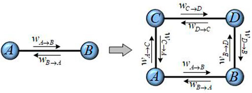
FIGURE 1. DWEI transformation of edge e = AB.

Let $\vec{G}(t)$ be the DWEI-network after t time steps; we generated a DWEI-network model, according to Algorithm 1. For the initial time step, the network $\vec{G}(0)$ is composed of an edge connect two nodes are labeled 1 and 2; set w_1→2 = w_2→1 = 1. When t ≥ 1, the DWEI-transformation is performed on every edge that exists in $\vec{G}(t-1)$, and this process continues until the network reaches the desired size. Figures 2, 3 show the DWEI-network at four-time steps t = 0, 1, 2, 3.

FIGURE 2

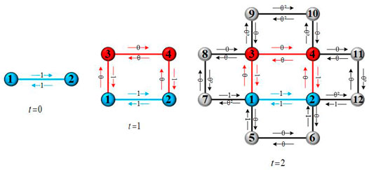
FIGURE 2. DWEI network at t =0, 1, 2.

FIGURE 3

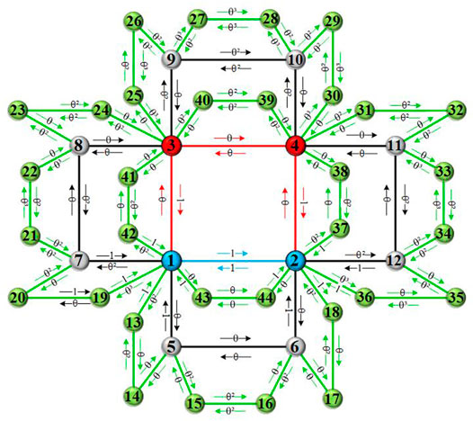
FIGURE 3. DWEI network at t = 3.

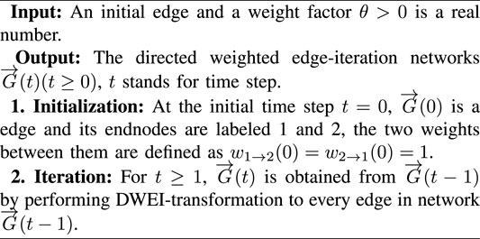
Algorithm 1. DWEI-network construction algorithm.

The out-strength of node i at time step t is defined as the sum of all weights of the edges starting from node i in −˗G(t), denoted as s + i (t) = PNt j=1 wi˗j (t). Meanwhile, the in-strength of node i represents the sum of the weights of all edges whose terminating nodes are i, expressed as s − i (t) = PNt j=1 wj˗i(t). The growth pattern determined by the node of network allows us to calculate the total number of nodes in −˗G(t) is Nt = 2 3 (4t + 2). Let ki(t) be the degree of a node i in network −˗G(t), the relationship between the degree of node i is ki(t) = 2ki(t − 1) in two consecutive time steps t − 1 and t. We can also get s + i (t) = (1 + Θ) t−ti+1 according to the definition of s+i(t), ti represents the time step when node i joined the network.

4 ATT for Weighted Walks

Different from the method of calculating the ATT by eigenvalues [25, 26], we derived a relationship governing the evolution for $T_i^{(t)}$ at generation t, according to the construction process of DWEI networks. Let Ω_t denote the set of all nodes in $\vec{G}(t)$; in order to clearly describe all the nodes in the derivation of the ATT, we divided the nodes in $\vec{G}(t)$ into two categories; the nodes that join the network at a time step t in $\vec{G}(t)$ are called new nodes, denoted by ${\widehat{\mathrm{\Omega }}}_t$; the nodes that join the network at a time step t − 1 and before are called old nodes, denoted as Ω_t−1.

Lemma 1. For the weighted walks of the DWEI network $\vec{G}(t+1)$, let θ > 0 be its weight factor, and the mean first passage time of any node i ∈ Ω_t satisfies the recursive relation

$T_i^{\left(t+1\right)}=\left(1+2\theta \right)T_i^{\left(t\right)}.(6)$

Proof. : The mean first-passage time between any two nodes in the DWEI network can be divided into the following three categories, and their simplified representation is as follows. Let X be the MFPT starting from the node i to any of its k_i(t − 1) old neighbors, which are directly connected to node i at the time step t − 1. Y represents the MFPT from any of k_i(t − 1) new neighbors of node i to one of its k_i(t − 1) old neighbors, and Z is the MFPT for starting from others new neighbors other than the aforementioned new nodes of node i to one of its k_i(t − 1) old neighbors. Thus, considering two consecutive time steps, we found that X, Y, Z satisfy the following equations:

$\left\{\begin{array}{cc}\hfill & X=\frac{1}{1+\theta }+\frac{\theta }{1+\theta }\left(1+Y\right),\hfill \\ \hfill & Y=\frac{1}{1+\theta }\left(1+X\right)+\frac{\theta }{1+\theta }\left(1+Z\right),\hfill \\ \hfill & Z=\frac{1}{1+\theta }+\frac{\theta }{1+\theta }\left(1+Y\right).\hfill \end{array}\right.(7)$

We get a solution X = 1 + 2θ by solving the aforementioned formula; it means that from the time step t to the next time t + 1, the trapping time for an arbitrary node i increases 1 + 2θ times the previous moment, that is, $T_i^{(t+1)}=(1+2\theta )T_i^{(t)}$. Owing to the network, $\vec{G}(t+1)$ is obtained by the network $\vec{G}(t)$ iteratively, so the relationship shown in Eq.6 is important in deriving the exact solution of ATT. □The sum of $T_i^{(t)}$ for all nodes in $\vec{G}(t)$ is recorded as $T_{t,tot}^{(t)}$. In addition, we also proposed intermediary quantities for 1 ≤ τ ≤ t; the sum of the MFPT of all nodes at time step τ is denoted as

$T_{\tau ,tot}^{\left(t\right)}=\sum _{i\in {\mathrm{\Omega }}_{\tau }}{T}_i^{\left(t\right)},(8)$

and the sum of the MFPT of all new nodes at a time step τ is formulated as

${\widehat{T}}_{\tau ,tot}^{\left(t\right)}=\sum _{i\in {\widehat{\mathrm{\Omega }}}_{\tau }}{T}_i^{\left(t\right)}.(9)$

Then, the average trapping time ⟨T⟩_t of the DWEI network $\vec{G}(t)$ is given by the following formula:

${⟨T⟩}_t=\frac{1}{N_t-1}\sum _{i=2}^{N_t}{T}_i^{\left(t\right)}=\frac{1}{N_t-1}{T}_{t,tot}^{\left(t\right)}.(10)$

Theorem 2. For the weighted random walks, N_t is the DWEI network order, let θ > 0 be the weight factor and t be the time step, then

(1) For $\theta =\frac{3}{2}$, the ATT of the DWEI network is

${⟨T⟩}_t=\frac{3}{2\times 4^t+1}\left[4^{t-1}\left(\frac{5}{3}t+\frac{154}{9}\right)+\frac{11}{18}\times 16^t\right].(11)$

The dominating term of ⟨T⟩_t is ⟨T⟩_t ∼ N_t for t → ∞.

(2) When $\theta \ne \frac{3}{2}$, the ATT of the DWEI network is

$\begin{array}{cc}\hfill {⟨T⟩}_t& =\frac{3}{2\times 4^t+1}\left\{\frac{{\left(1+2\theta \right)}^{t-2}}{6\theta \left(2\theta -3\right)}\left[\left(48+6\times 4^{t+1}\right){\theta }^4\right.\right.\hfill \\ \hfill & +\left(16-4^{t+1}\right){\theta }^3+\left(-20+34\times 4^t\right){\theta }^2\hfill \\ \hfill & \left.\left.+\left(-8-19\times 4^t\right)\theta -3\times 4^t\right]\right\},\hfill \end{array}(12)$

the relationship between ⟨T⟩_t and the network order N_t satisfy ${⟨T⟩}_t\sim N_t^{{\log }_4(1+2\theta )}$ for t → ∞.

Proof. It can be seen that the problem for evaluating ⟨T⟩_t is reduced to determining $T_{t,tot}^{(t)}$ from Eq.10. We considered the MFPT of all nodes in the light of the classification of new nodes and old nodes, which is written as the following formula:

$\begin{array}{cc}\hfill T_{t,tot}^{\left(t\right)}& =T_{t-1,tot}^{\left(t\right)}+{\widehat{T}}_{t,tot}^{\left(t\right)}\hfill \\ \hfill & =\left(1+2\theta \right)T_{t-1,tot}^{\left(t-1\right)}+{\widehat{T}}_{t,tot}^{\left(t\right)}.\hfill \end{array}(13)$

Obviously, once we calculated the result of ${\widehat{T}}_{t,tot}^{(t)}$ about the new nodes, we can obtain a recursive equation for $T_{t,tot}^{(t)}$.Referring to the DWEI transformation of all edges in the network, we found that each new node must have two neighbors for the nodes in ${\widehat{\mathrm{\Omega }}}_t$; one of the two neighbors is a new node generated at the time step t, and the other is an old node added before the time step t. There are two new nodes in the next time step for each edge e = uv; we labeled them as x₁ and x₂, respectively. If the MFPTs of the four nodes u, v, x₁, x₂ at a certain moment are expressed as T(u), T(v), T (x₁), T (x₂), the relationships between the MFPTs of new nodes x₁, x₂ and its neighbors can be derived as

$\left\{\begin{array}{cc}\hfill & T\left(x_1\right)=\frac{1}{1+\theta }\left(1+T\left(u\right)\right)+\frac{\theta }{1+\theta }\left(1+T\left(x_2\right)\right),\hfill \\ \hfill & T\left(x_2\right)=\frac{1}{1+\theta }\left(1+T\left(v\right)\right)+\frac{\theta }{1+\theta }\left(1+T\left(x_1\right)\right).\hfill \end{array}\right.(14)$

Combining the two formulas in Eq. 14, we can get

$T\left(x_1\right)+T\left(x_2\right)=2\left(1+\theta \right)+T\left(u\right)+T\left(v\right).(15)$

For the DWEI network corresponding to the first few time steps, since the number of nodes in the network is small, we can directly calculate the value of ${\widehat{T}}_{i,tot}^{(i)}$ and $T_{i,tot}^{(i)}$ for 0 ≤ i ≤ t. For example, when t = 1, the way to obtain the value of ${\widehat{T}}_{1,tot}^{(1)}$ and $T_{1,tot}^{(1)}$ is as follows: we first listed the relations between the four nodes in $\vec{G}(1)$. There are a total of four nodes in $\vec{G}(1)$: node 1 is set as a trap, so we have $T_1^{(1)}=0$, and the out-degree of node 2 is 1 + θ. The weights on its edges to node 1 and node 4 are 1 and 0, respectively; then, the second equation in Eq.16 holds, the equations related to node 3 and 4 can be obtained similarly.

$\left\{\begin{array}{cc}\hfill & T_1^{\left(1\right)}=0,\hfill \\ \hfill & T_2^{\left(1\right)}=\frac{1}{1+\theta }\left(1+T_1^{\left(1\right)}\right)+\frac{\theta }{1+\theta }\left(1+T_4^{\left(1\right)}\right),\hfill \\ \hfill & T_3^{\left(1\right)}=\frac{1}{1+\theta }\left(1+T_1^{\left(1\right)}\right)+\frac{\theta }{1+\theta }\left(1+T_4^{\left(1\right)}\right),\hfill \\ \hfill & T_4^{\left(1\right)}=\frac{1}{1+\theta }\left(1+T_2^{\left(1\right)}\right)+\frac{\theta }{1+\theta }\left(1+T_3^{\left(1\right)}\right).\hfill \end{array}\right.(16)$

Among the four nodes, the two nodes labeled 1 and 2 are called old nodes, and 3 and 4 are called new nodes; thus, the sum of MFPTs of all new nodes is equal to

$\begin{array}{cc}\hfill {\widehat{T}}_{1,tot}^{\left(1\right)}& =\sum _{i\in {\widehat{\mathrm{\Omega }}}_1}{T}_i^{\left(t\right)}=T_3^{\left(1\right)}+T_4^{\left(1\right)}\hfill \\ \hfill & =4\theta +3=2\left(1+\theta \right)+{\widehat{T}}_{0,tot}^{\left(1\right)}.\hfill \end{array}(17)$

Therefore, the sum of MFPTs of all nodes in the network $\vec{G}(1)$ can be expressed as

$\begin{array}{cc}\hfill T_{1,tot}^{\left(1\right)}& =T_1^{\left(1\right)}+T_2^{\left(1\right)}+T_3^{\left(1\right)}+T_4^{\left(1\right)}\hfill \\ \hfill & =6\theta +4.\hfill \end{array}(18)$

Considering Eq. 15 and summing this equation over all new nodes in ${\widehat{\mathrm{\Omega }}}_t$, then we obtain

$\begin{array}{cc}\hfill {\widehat{T}}_{t,tot}^{\left(t\right)}& =\sum _{i\in {\widehat{\mathrm{\Omega }}}_t}{T}_i^{\left(t\right)}=\left(1+\theta \right)|{\widehat{\mathrm{\Omega }}}_t|+\sum _{i\in {\mathrm{\Omega }}_{t-1}}\left[k_i\left(t-1\right)\times T_i^{\left(t\right)}\right]\hfill \\ \hfill & =2\left(1+\theta \right)\times 4^{t-1}+2{\widehat{T}}_{t-1,tot}^{\left(t\right)}+2^2{\widehat{T}}_{t-2,tot}^{\left(t\right)}+\cdots \hfill \\ \hfill & +2^{t-1}{\widehat{T}}_{1,tot}^{\left(t\right)}+2^t{\widehat{T}}_{0,tot}^{\left(t\right)}.\hfill \end{array}(19)$

Similarly, the following equation about ${\widehat{T}}_{t+1,tot}^{(t+1)}$ is also valid; refer to Eq.19

$\begin{array}{cc}\hfill {\widehat{T}}_{t+1,tot}^{\left(t+1\right)}& =2\left(1+\theta \right)\times 4^t+2{\widehat{T}}_{t,tot}^{\left(t+1\right)}+2^2{\widehat{T}}_{t-1,tot}^{\left(t+1\right)}+\cdots \hfill \\ \hfill & +2^t{\widehat{T}}_{1,tot}^{\left(t+1\right)}+2^{t+1}{\widehat{T}}_{0,tot}^{\left(t+1\right)}.\hfill \end{array}(20)$

Then, subtracting the product of Eq.19 multiplied by 2 (1 + 2θ) from Eq. 20, we have

$\begin{array}{cc}\hfill & {\widehat{T}}_{t+1,tot}^{\left(t+1\right)}-2\left(1+2\theta \right){\widehat{T}}_{t,tot}^{\left(t\right)}\hfill \\ \hfill & =2\left(1+\theta \right)\times 4^t-4^t\left(1+\theta \right)\left(1+2\theta \right)\hfill \\ \hfill & +2\left(1+2\theta \right){\widehat{T}}_{t,tot}^{\left(t\right)}.\hfill \end{array}(21)$

After merging ${\widehat{T}}_{t,tot}^{(t)}$ on both sides of Eq. 21, we get the following recursive relation:

${\widehat{T}}_{t+1,tot}^{\left(t+1\right)}=4\left(1+2\theta \right){\bar{T}}_{t,tot}^{\left(t\right)}+4^t\left(1+\theta \right)\left(1-2\theta \right).(22)$

Considering a value ${\widehat{T}}_{1,tot}^{(1)}=4\theta +3$ that we have already solved as an initial condition, a closed-form solution of Eq.22 can be derived:

$\begin{array}{cc}\hfill {\widehat{T}}_{t,tot}^{\left(t\right)}& =\frac{6{\theta }^2+5\theta +1}{2\theta }\times {\left[4\left(1+2\theta \right)\right]}^{t-1}\hfill \\ \hfill & -\frac{\left(1+\theta \right)\left(1-2\theta \right)}{2\theta }\times 4^{t-1}.\hfill \end{array}(23)$

1) For $\theta =\frac{3}{2}$, we get ${\widehat{T}}_{t,tot}^{(t)}=\frac{22}{3}\times 16^{t-1}+\frac{5}{3}\times 4^{t-1}$. Substituting this equation and $\theta =\frac{3}{2}$ into Eq. 13, we get

$T_{t,tot}^{\left(t\right)}=\left(\frac{5}{3}t-\frac{22}{3}\right)\times 4^{t-1}+\frac{88}{9}\left(16^{t-1}-4^{t-1}\right).(24)$

We can get $t={\log }_4(\frac{3}{2}{N}_t-2)$ from $N_t=\frac{2}{3}(4^t+2)$. Considering Eq. 10, we obtain the result shown in Eq.11:

$\begin{array}{cc}\hfill {⟨T⟩}_t& =\frac{3}{2\times 4^t+1}\left[4^{t-1}\left(\frac{5}{3}t+\frac{154}{9}\right)+\frac{11}{18}\times 16^t\right]\hfill \\ \hfill & \sim N_t.\hfill \end{array}(25)$

2) When $\theta \ne \frac{3}{2}$, the sum of MFPT of all nodes satisfies the following recurrence relation:

$\begin{array}{cc}\hfill T_{t,tot}^{\left(t\right)}& =\left(1+2\theta \right)T_{t-1,tot}^{\left(t-1\right)}+{\widehat{T}}_{t,tot}^{\left(t\right)}\hfill \\ \hfill & =\left(1+2\theta \right)T_{t-1,tot}^{\left(t-1\right)}+\left(4\theta +3\right){\left[4\left(1+2\theta \right)\right]}^{t-1}\hfill \\ \hfill & +\frac{4^{t-1}\left(1+\theta \right)\left(1-2\theta \right)}{2\theta }\left[{\left(1+2\theta \right)}^{t-1}-1\right].\hfill \end{array}(26)$

With the help of a condition $T_{1,tot}^{(1)}=6\theta +4$ in Eq. 18, then Eq.26 is resolved to obtain a solution about $T_{t,tot}^{(t)}$:

$\begin{array}{cc}\hfill T_{t,tot}^{\left(t\right)}& =\frac{{\left(1+2\theta \right)}^{t-2}}{6\theta \left(2\theta -3\right)}\left[\left(48+6\times 4^{t+1}\right){\theta }^4+\left(16-4^{t+1}\right){\theta }^3\right.\hfill \\ \hfill & +\left(34\times 4^t-20\right){\theta }^2-\left(8+19\times 4^t\right)\theta \hfill \\ \hfill & \left.3\times 4^t\right].\hfill \end{array}(27)$

Furthermore, substituting Eq.27 into Eq. 10, we get the average of all MFPTs in the network $\vec{G}(t)$:

$\begin{array}{cc}\hfill {⟨T⟩}_t& =\frac{1}{N_t-1}{T}_{t,tot}^{\left(t\right)}\hfill \\ \hfill & =\frac{3}{2\times 4^t+1}\left\{\frac{{\left(1+2\theta \right)}^{t-2}}{6\theta \left(2\theta -3\right)}\left[\left(48+6\times 4^{t+1}\right){\theta }^4\right.\right.\hfill \\ \hfill & +\left(16-4^{t+1}\right){\theta }^3+\left(-20+34\times 4^t\right){\theta }^2\hfill \\ \hfill & \left.\left.+\left(-8-19\times 4^t\right)\theta -3\times 4^t\right]\right\}.\hfill \end{array}(28)$

Actually, the DWEI network can be regarded as a binary network for a special case θ = 1; based on this situation, the value of ⟨T⟩_t we obtained is consistent with the result in the literature [27]. Next, we showed how to express ⟨T⟩_t in terms of the network order N_t; Substituting $t={\log }_4(\frac{3}{2}{N}_t-2)$ into Eq. 28, then we have

$\begin{array}{cc}\hfill {⟨T⟩}_t& \approx \frac{24{\theta }^4-4{\theta }^3+34{\theta }^2-19\theta -3}{\left(12{\theta }^2-18\theta \right){\left(1+2\theta \right)}^2}{\left(\frac{3}{2}{N}_t\right)}^{{\log }_4\left(1+2\theta \right)}\hfill \\ \hfill & \sim {\left(N_t\right)}^{{\log }_4\left(1+2\theta \right)},\hfill \end{array}(29)$

as t → ∞. According to Eq. 29, we found that the weight θ can not only modify the pre-factor of ⟨T⟩_t but also the scaling log₄ (1 + 2θ) of ⟨T⟩_t. In addition, we can obtain the following conclusions in weighted random walks by analyzing Eqs 25, 29, when $\theta =\frac{3}{2}$, ⟨T⟩_t grows linearly with N_t; however, ⟨T⟩_t grows sub-linearly and super-linearly with the network order N_t for $\theta <\frac{3}{2}$ and $\theta >\frac{3}{2}$, respectively; the results are shown in Figure 4.

FIGURE 4

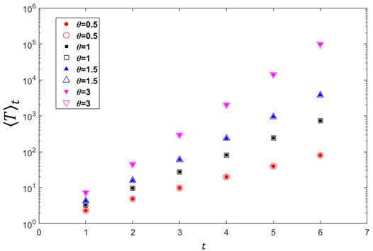
FIGURE 4. Solids indicate the numerical results, and the hollows indicate the results of our analytical results.

5 ATT for Delayed Weighted Walks

In this section, a delay probability 0 ≤ p ≤ 1 is introduced to explore its impact on the ATT of our network in the weighted random walk with delay [28]. The delayed weighted random walk is defined as follows; for delay probability 0 ≤ p ≤ 1, the walker in network $\vec{G}(t-1)$ is allowed to move to any neighbor either in $\vec{G}(t-1)$ or in $\vec{G}(t)$ with probability p and 1 − p, respectively, which is the transition probability p_ij for the walker jumping from node i to another node j and is formulated as

$p_{ij}=\left\{\begin{array}{cccc}\hfill & p\times \frac{w_{i\to j}\left(t\right)}{s_i^{+}\left(t-1\right)}\hfill & \hfill ,& i\in {\mathrm{\Omega }}_{t-1},j\in {\mathrm{\Omega }}_{t-1},\hfill \\ \hfill & \left(1-p\right)\times \frac{w_{i\to j}\left(t\right)}{s_i^{+}\left(t\right)}\hfill & \hfill ,& i\in {\mathrm{\Omega }}_{t-1},j\in {\widehat{\mathrm{\Omega }}}_t,\hfill \\ \hfill & \frac{w_{i\to j}\left(t\right)}{s_j^{+}\left(t\right)}\hfill & \hfill ,& \text{if}i\in {\widehat{\mathrm{\Omega }}}_t,j\in {\mathrm{\Omega }}_t.\hfill \end{array}\right.(30)$

The two special cases of delayed weighted random walks are as follows:

1) When p = 0, delayed weighted random walks reduce to regular weighted random walks discussed in the previous section because the walker moves from node i to any neighboring node j with transition probability $p_{ij}(t)=\frac{w_{i\to j}(t)}{s_i^{+}(t)}$.

2) When p = 1, if node i is created before the time step t, then the walker jumping from the current node i to any neighboring node j in $\vec{G}(t-1)$ with the transition probability $p_{ij}(t)=\frac{w_{i\to j}(t)}{s_i^{+}(t-1)}$. Otherwise, the walker moves from the current node i to any neighbor node j on $\vec{G}(t)$ with the transition probability $p_{ij}(t)=\frac{w_{i\to j}(t)}{s_i^{+}(t)}$.

Lemma 3. For the delayed weighted random walks of the DWEI network $\vec{G}(t+1)$; let θ > 0 be a weight factor and 0 ≤ p ≤ 1 represents a delay probability, $T_i^{(t)}$ is the MFPT corresponding to the regular weighted random walks; the relationship between MFPT $F_i^{(t+1)}$ of delayed weighted random walks and $T_i^{(t)}$ for node i is

$F_i^{\left(t+1\right)}=\frac{\left(2-2p\right){\theta }^2+\left(p+3\right)\theta +1}{\theta -\theta p+1}{T}_i^{\left(t\right)}.(31)$

Proof. : Let $F_i^{(t)}$ be the MFPT in the delayed weighted random walks, similar to the study of weighted random walks, we classified all the nodes according to the type of walks. The definition of three quantities X, Y, and Z is the same as section 4, and they satisfy the following three equations in the delayed weighted random walks:

$\left\{\begin{array}{cc}\hfill & X=p+\left(1-p\right)\left[\frac{1}{1+\theta }+\frac{\theta }{1+\theta }\left(1+Y\right)\right],\hfill \\ \hfill & Y=\frac{1}{1+\theta }\left(1+X\right)+\frac{\theta }{1+\theta }\left(1+Z\right),\hfill \\ \hfill & Z=\frac{1}{1+\theta }+\frac{\theta }{1+\theta }\left(1+Y\right).\hfill \end{array}\right.(32)$

The solved X involves the delay probability p and the weight factor θ; its expression is

$X=\frac{\left(2-2p\right){\theta }^2+\left(p+3\right)\theta +1}{\theta -\theta p+1}.(33)$

Therefore, we have deduced the relationship between $F_i^{(t+1)}$ and $T_i^{(t)}$, as shown in Eq.31.

Theorem 4. For the delayed weighted random walks, let θ > 0 and t ≥ 0 be the weight factor and time step, N_t is the DWEI-network order; then, the exact dependence of ATT on the network order N_t is as follows:

(1) For $\theta =\frac{3}{2}$,

$\begin{array}{cc}\hfill {⟨F⟩}_t& \approx \left[\frac{110-33p}{144\left(5-3p\right)}+\frac{110-33p}{16\left(15-9p\right)}\right]N_t\hfill \\ \hfill & \sim N_t.\hfill \end{array}(34)$

2) When $\theta \ne \frac{3}{2}$,

${⟨F⟩}_t\sim N_t^{{\log }_4\left(1+2\theta \right)}.(35)$

for t → ∞.

Proof. : We defined ⟨F⟩_t as the ATT for delayed weighted random walks in the network $\vec{G}(t)$; in order to obtain the closed-form solution of ⟨F⟩_t, two quantities $F_{\tau ,tot}^{(t)}={\sum }_{i\in {\mathrm{\Omega }}_{\tau }}{F}_i^{(t)}$ and ${\widehat{F}}_{\tau ,tot}^{(t)}={\sum }_{i\in {\widehat{\mathrm{\Omega }}}_{\tau }}{F}_i^{(t)}$ are proposed for the time step τ ≤ t. Extending Eq.10 to the delayed weighted random walks, a formula about ⟨F⟩_t is as follows:

${⟨F⟩}_t=\frac{1}{N_t-1}{F}_{t,tot}^{\left(t\right)}.(36)$

The sum of MFPT of all nodes in the network is composed of the sum of MFPT of old nodes and new nodes; it can be formulated as

$\begin{array}{cc}\hfill F_{t,tot}^{\left(t\right)}& =F_{t-1,tot}^{\left(t\right)}+{\widehat{F}}_{t,tot}^{\left(t\right)}\hfill \\ \hfill & =\frac{\left(2-2p\right){\theta }^2+\left(p+3\right)\theta +1}{\theta -\theta p+1}{T}_{t-1,tot}^{\left(t-1\right)}+{\widehat{F}}_{t,tot}^{\left(t\right)}.\hfill \end{array}(37)$

Similar to the calculation of Eqs 13, 17, it shows that our calculation focuses on solving ${\widehat{F}}_{t,tot}^{(t)}$; we specified the sum of MFPT of all new nodes as

$\begin{array}{cc}\hfill {\widehat{F}}_{t,tot}^{\left(t\right)}& =\left(1+\theta \right)|{\widehat{\mathrm{\Omega }}}_t|+\sum _{i\in {\widehat{\mathrm{\Omega }}}_{t-1}}\left[k_i\left(t-1\right)\right.\hfill \\ \hfill & \left.\times \frac{\left(2-2p\right){\theta }^2+\left(p+3\right)\theta +1}{\theta -\theta p+1}{T}_i^{\left(t-1\right)}\right].\hfill \end{array}(38)$

We can directly get ${\widehat{F}}_{t+1,tot}^{(t+1)}$, according to the aforementioned equation for time step t + 1:

$\begin{array}{cc}\hfill {\widehat{F}}_{t+1,tot}^{\left(t+1\right)}& =\left(1+\theta \right)|{\widehat{\mathrm{\Omega }}}_{t+1}|+\sum _{i\in {\widehat{\mathrm{\Omega }}}_t}\left[k_i\left(t\right)\right.\hfill \\ \hfill & \left.\times \frac{\left(2-2p\right){\theta }^2+\left(p+3\right)\theta +1}{\theta -\theta p+1}{T}_i^{\left(t\right)}\right].\hfill \end{array}(39)$

Multiplying Eq.38 with 2 (1 + 2θ) and subtracting the result from Eq. 39, we derived the recursive connection between ${\widehat{F}}_{t+1,tot}^{(t+1)}$ and ${\widehat{F}}_{t,tot}^{(t)}$ from the results obtained:

$\begin{array}{cc}\hfill & {\widehat{F}}_{t+1,tot}^{\left(t+1\right)}-2\left(1+2\theta \right){\widehat{F}}_{t,tot}^{\left(t\right)}\hfill \\ \hfill & =\left(1+\theta \right)\left[|{\widehat{\mathrm{\Omega }}}_{t+1}|-2\left(1+2\theta \right)|{\widehat{\mathrm{\Omega }}}_t|\right]\hfill \\ \hfill & +2\times \frac{\left(2-2p\right){\theta }^2+\left(p+3\right)\theta +1}{\theta -\theta p+1}\sum _{i\in {\widehat{\mathrm{\Omega }}}_t}{T}_i^{\left(t\right)},\hfill \end{array}(40)$

where ${\sum }_{i\in {\widehat{\mathrm{\Omega }}}_t}{T}_i^{(t)}={\widehat{T}}_{t,tot}^{(t)}$ is obvious, and the number of nodes newly added to the network at the time step t is $|{\widehat{\mathrm{\Omega }}}_t|=2\times 4^{t-1}$, plugging Eq.23 into Eq. 40, and combining a condition ${\widehat{F}}_{1,tot}^{(1)}=\frac{1}{\theta p+\theta +1}[4{\theta }^2+(7+p)\theta +3]$, then

$\begin{array}{cc}\hfill {\widehat{F}}_{t,tot}^{\left(t\right)}& ={\left(2+4\theta \right)}^{t-1}\times \frac{4{\theta }^2+\left(7+p\right)\theta +3}{\theta p+\theta +1}+\frac{1}{{\theta }^2-p{\theta }^2+\theta \left.\right)}\hfill \\ \hfill & \times \left[\left(4p-4\right){\theta }^4+\left(4p-4\right){\theta }^3+\left(3-p\right){\theta }^2+\left(2-p\right)\theta \right.\hfill \\ \hfill & \left.-1\right]\times \frac{1}{2\theta -1}\left[{\left(2+4\theta \right)}^{t-2}\times \left(1+2\theta \right)-2\times 4^{t-2}\right]\hfill \\ \hfill & +\frac{1}{{\theta }^2-{\theta }^{2}p+\theta }\left[\left(12-12p\right){\theta }^4+\left(28-4p\right){\theta }^3\right.\hfill \\ \hfill & \left.+\left(3p+23\right){\theta }^2+\left(p+8\right)\theta +1\right]\hfill \\ \hfill & \times \frac{{\left(4+8\theta \right)}^{t-1}-{\left(2+4\theta \right)}^{t-1}}{2+4\theta }.\hfill \end{array}(41)$

1) When the weight factor satisfies $\theta =\frac{3}{2}$, we obtain

$\begin{array}{cc}\hfill {\widehat{F}}_{t,tot}^{\left(t\right)}& =\frac{3p+45}{3p+5}\times 8^{t-1}+\frac{4\left(30p-25\right)}{15-9p}\times \left(2\times 8^{t-2}-4^{t-2}\right)\hfill \\ \hfill & +\frac{\left(110-33p\right)\left(16^{t-1}-8^{t-1}\right)}{15-9p}.\hfill \end{array}(42)$

In this case, we can calculate the sum of MFPT of all nodes by combining Eqs 24, 37, 42:

$\begin{array}{cc}\hfill F_{t,tot}^{\left(t\right)}& =\frac{2\left(10-3p\right)}{5-3p}\left[\left(\frac{5}{3}t-9\right)\times 4^{t-2}+\frac{88\left(16^{t-2}-4^{t-2}\right)}{9}\right]\hfill \\ \hfill & +\frac{3p+45}{3p+5}\times 8^{t-1}+\left(\frac{120p-100}{15-9p}\right)\left(2\times 8^{t-2}-4^{t-2}\right)\hfill \\ \hfill & +\frac{\left(110-33p\right)\left(16^{t-1}-8^{t-1}\right)}{15-9p}.\hfill \end{array}(43)$

Substituting Eq.43 into Eq. 36, we can get the expression of ⟨F⟩_t. Furthermore, we deduce that the trend of ⟨F⟩_t increases with N_t for a large network:

$\begin{array}{cc}\hfill {⟨F⟩}_t& =\frac{1}{N_t-1}{F}_{t,tot}^{\left(t\right)}\hfill \\ \hfill & \approx \left[\frac{110-33p}{144\left(5-3p\right)}+\frac{110-33p}{16\left(15-9p\right)}\right]N_t\hfill \\ \hfill & \sim N_t.\hfill \end{array}(44)$

The aforementioned formula shows that ⟨F⟩_t increases linearly with N_t when $\theta =\frac{3}{2}$.2) For $\theta \ne \frac{3}{2}$, plugging Eq.41 into Eq. 37, we have obtained the analytical formula of $F_{t,tot}^{(t)}$. For simplicity, we replaced the three coefficients with A, B, and C, respectively, which are all controlled by the weight factor θ and have no dependencies on the time step t.

$\begin{array}{cc}\hfill F_{t,tot}^{\left(t\right)}& =A{\left(1+2\theta \right)}^{t-3}\times \left[4^t\left(6{\theta }^4-{\theta }^3+\frac{17}{2}{\theta }^2-\frac{19}{4}\theta -\frac{3}{4}\right)\right.\hfill \\ \hfill & \left.+48{\theta }^4+16{\theta }^3-20{\theta }^2-8\theta \right]+2^{t-1}{\left(1+2\theta \right)}^{t-1}\hfill \\ \hfill & \times \frac{4{\theta }^2+\left(7+p\right)\theta +3}{\theta p+\theta +1}+\frac{B}{2\theta -1}\left[2^{t-2}{\left(1+2\theta \right)}^{t-1}\right.\hfill \\ \hfill & \left.-2\times 4^{t-1}\right]+C\times \frac{\left(4^{t-1}-2^{t-1}\right){\left(1+2\theta \right)}^t}{2{\left(1+2\theta \right)}^2}.\hfill \end{array}(45)$

Among them, three variables A, B, C equal to

$\begin{array}{cc}\hfill A& =\frac{\left(2-2p\right){\theta }^2+\left(p+3\right)\theta +1}{6\theta \left(2\theta -3\right)\left(\theta -\theta p+1\right)},\hfill \\ \hfill B& =\frac{1}{{\theta }^2-p{\theta }^2+\theta }\left[\left(4p-1\right){\theta }^4+\left(4p-4\right){\theta }^3\right.\hfill \\ \hfill & \left.+\left(3-p\right){\theta }^2+\left(2-p\right)\theta -1\right],\hfill \\ \hfill C& =\frac{1}{{\theta }^2-p{\theta }^2+\theta \left.\right)}\left[\left(12-12p\right){\theta }^4+\left(28-4p\right){\theta }^3\right.\hfill \\ \hfill & \left.+\left(3p+23\right){\theta }^2+\left(p+8\right)\theta +1\right].\hfill \end{array}(46)$

Next, we gave the average of MFPT for all nodes except the trap node; substituting Eq.45 into Eq. 36, we obtain

$\begin{array}{cc}\hfill {⟨F⟩}_t& =\frac{1}{N_t-1}{F}_{t,tot}^{\left(t\right)}\hfill \\ \hfill & =\frac{3}{2\times 4^t+1}\left\{A{\left(1+2\theta \right)}^{t-3}\times \left[4^t\left(6{\theta }^4-{\theta }^3+\frac{17}{2}{\theta }^2\right.\right.\right.\hfill \\ \hfill & \left.\left.-\frac{19}{4}\theta -\frac{3}{4}\right)+48{\theta }^4+16{\theta }^3-20{\theta }^2-8\theta \right]\hfill \\ \hfill & +2^{t-1}{\left(1+2\theta \right)}^{t-1}\times \frac{4{\theta }^2+\left(7+p\right)\theta +3}{\theta p+\theta +1}\hfill \\ \hfill & +\frac{B}{2\theta -1}\left[2^{t-2}{\left(1+2\theta \right)}^{t-1}-2\times 4^{t-1}\right]\hfill \\ \hfill & \left.+C\times \frac{\left(4^{t-1}-2^{t-1}\right){\left(1+2\theta \right)}^t}{2{\left(1+2\theta \right)}^2}\right\}.\hfill \end{array}(47)$

Considering $t={\log }_4(\frac{3}{2}{N}_t-2)$, the expression of ⟨F⟩_t in Eq.47 can be represented in terms of the network order N_t in the following form:

$\begin{array}{cc}\hfill {⟨F⟩}_t& =\frac{1}{N_t-1}\left\{\frac{A}{{\left(1+2\theta \right)}^3}{\left(\frac{3}{2}{N}_t-2\right)}^{{\log }_4\left(1+2\theta \right)}\right.\hfill \\ \hfill & \times \left[\left(\frac{3}{2}{N}_t-2\right)\left(6{\theta }^4-{\theta }^3+\frac{17}{2}{\theta }^2-\frac{19}{4}\theta -\frac{3}{4}\right.\right.\hfill \\ \hfill & \left.\left.+48{\theta }^4+16{\theta }^3-20{\theta }^2-8\theta \right)\right]+\frac{1}{2\left(1+2\theta \right)}\hfill \\ \hfill & \times {\left(\frac{3}{2}{N}_t-2\right)}^{{\log }_4\left(1+2\theta \right)+\frac{1}{2}}\times \frac{4{\theta }^2+\left(7+p\right)\theta +3}{\theta p+\theta +1}\hfill \\ \hfill & +\frac{B}{2\theta -1}\left[\frac{1}{4\left(1+2\theta \right)}{\left(\frac{3}{2}{N}_t-2\right)}^{{\log }_4\left(1+2\theta \right)+\frac{1}{2}}\right.\hfill \\ \hfill & \left.-\frac{1}{2}\left(\frac{3}{2}{N}_t-2\right)\right]+C\times \left.\right[[\frac{\frac{1}{4}{\left(\frac{3}{2}{N}_t-2\right)}^{1+{\log }_4\left(1+2\theta \right)}}{2{\left(1+2\theta \right)}^2}\hfill \\ \hfill & \left.-\frac{\frac{1}{2}{\left(\frac{3}{2}{N}_t-2\right)}^{\frac{1}{2}+{\log }_4\left(1+2\theta \right)}}{2{\left(1+2\theta \right)}^2}]\right\}.\hfill \end{array}(48)$

For a large t, we have the following expression for the dominating term of ⟨F⟩_t:

$\begin{array}{cc}\hfill {⟨F⟩}_t& \approx \left[\frac{A\left(6{\theta }^4-{\theta }^3+\frac{17}{2}{\theta }^2-\frac{19}{4}\theta -\frac{3}{4}\right)}{{\left(1+2\theta \right)}^3}+\frac{C}{8{\left(1+2\theta \right)}^2}\right]\hfill \\ \hfill & \times {\left(\frac{3}{2}{N}_t-2\right)}^{{\log }_4\left(1+2\theta \right)}\hfill \\ \hfill & \sim N_t^{{\log }_4\left(1+2\theta \right)}.\hfill \end{array}(49)$

Therefore, Eq.49 shows that ⟨F⟩_t grows sub-linearly and super-linearly with the network size, when $\theta <\frac{3}{2}$ and $\theta >\frac{3}{2}$,respectively; when $\theta =\frac{3}{2}$, we know that ⟨F⟩_t grows linearly with the network size from Eq.44. The coefficient $\frac{1}{{\left(1+2\theta \right)}^3}\left[A\left(6{\theta }^4-{\theta }^3+\frac{17}{2}{\theta }^2-\frac{19}{4}\theta -\frac{3}{4}\right)\right]+\frac{1}{8{\left(1+2\theta \right)}^2}\times C$ in Eq.49 is obviously affected by the delay probability p and the weight factor θ. However, the exponent log₄ (1 + 2θ) of N_t is only controlled by the weight factor θ and has no dependencies on the delay probability p. Also, we have known that the delay parameter p can only change the coefficient of the ATT; it has less influence on the trapping efficiency.

6 Conclusion

Based on the undirected unweighted network, we considered the weight and the out-degree and in-degree of nodes in complex systems. We proposed a network operator and a class of directed weighted edge-iteration networks and derived the closed form solution of the average trapping time of two different random walks with a given trap node; one of the random walks is based on the weight θ alone acting on the transition probability, and the other is the weight factor θ and delay parameter p impacting on the transition probability at the same time. The solution shows that the directed weighted construction has a significant effect on the trapping efficiency, and the leading scale of the ATT can be sub-linearly, linearly, and super-linearly with the network size when $\theta <\frac{3}{2}$, $\theta =\frac{3}{2}$, and $\theta >\frac{3}{2}$, respectively. In view of the importance of weight to control the efficiency of random walks, we can extend the undirected network to a directed weighted network or adjust the weights of the edges in the two directions of the directed network so as to achieve the purpose of modifying the weight. Our next goal is to reveal the influence of other factors in directed networks on random walks, such as both nodes and edges having weights. We need to find more variables that can control the trapping process in combination with the real network and give a guiding analytical process.

Data Availability Statement

The original contributions presented in the study are included in the article/Supplementary Material; further inquiries can be directed to the corresponding author.

Author Contributions

JS provided this topic and wrote the manuscript. MM and MZ discussed and drew all figures. BY modified and guided the manuscript. All authors contributed to the manuscript and approved the submitted version.

Funding

This research was supported by the National Key Research and Development Plan under the Grant No. 2019YFA0706401 and the National Natural Science Foundation of China under Grants Nos. 61872166 and 61662066, the Technological Innovation Guidance Program of Gansu Province: Soft Science Special Project (21CX1ZA285), and the Northwest China Financial Research Center Project of Lanzhou University of Finance and Economics (JYYZ201905).

Conflict of Interest

The authors declare that the research was conducted in the absence of any commercial or financial relationships that could be construed as a potential conflict of interest.

Publisher’s Note

All claims expressed in this article are solely those of the authors and do not necessarily represent those of their affiliated organizations, or those of the publisher, the editors and the reviewers. Any product that may be evaluated in this article, or claim that may be made by its manufacturer, is not guaranteed or endorsed by the publisher.

References

1. Hwang S, Lee DS, Kahng B. First Passage Time for Random Walks in Heterogeneous Networks. Phys Rev Lett (2012) 109(8):088701. doi:10.1103/PhysRevLett.109.088701

PubMed Abstract | CrossRef Full Text | Google Scholar

2. Bestehorn M, Riascos AP, Michelitsch TM, Collet BA. A Markovian Random Walk Model of Epidemic Spreading. Continuum Mech Thermodyn (2021) 33:1207–21. doi:10.1007/s00161-021-00970-z

CrossRef Full Text | Google Scholar

3. Shirsat A, Elamvazhuthi K, Berman S. Multi-Robot Target Search Using Probabilistic Consensus on Discrete Markov Chains. In: 2020 IEEE International Symposium on Safety, Security, and Rescue Robotics (SSRR). Abu Dhabi, UAE: IEEE (2020). doi:10.1109/ssrr50563.2020.9292589

CrossRef Full Text | Google Scholar

4. El Hadidy MAA. Generalised Linear Search Plan for a D-Dimensional Random Walk Target. Ijmor (2019) 15(2):211. doi:10.1504/ijmor.2019.10022970

CrossRef Full Text | Google Scholar

5. Blumen A, Zumofen G. Energy Transfer as a Random Walk on Regular Lattices. J Chem Phys (1981) 75:892–907. doi:10.1063/1.442086

CrossRef Full Text | Google Scholar

6. Sokolov IM, Mai J, Blumen A. Paradoxal Diffusion in Chemical Space for Nearest-Neighbor Walks over Polymer Chains. Phys Rev Lett (1997) 79:857–60. doi:10.1103/physrevlett.79.857

CrossRef Full Text | Google Scholar

7. Zhang Z, Julaiti A, Hou B, Zhang H, Chen G. Mean First-Passage Time for Random Walks on Undirected Networks. Eur Phys J B (2011) 84(4):691–7. doi:10.1140/epjb/e2011-20834-1

CrossRef Full Text | Google Scholar

8. LinZhang YZZ, Zhang Z. Random Walks in Weighted Networks with a Perfect Trap: an Application of Laplacian Spectra. Phys Rev E Stat Nonlin Soft Matter Phys (2013) 87(6):062140. doi:10.1103/PhysRevE.87.062140

PubMed Abstract | CrossRef Full Text | Google Scholar

9. Wu B, Zhang Z. Controlling the Efficiency of Trapping in Treelike Fractals. J Chem Phys (2013) 139(2):024106. doi:10.1063/1.4812690

PubMed Abstract | CrossRef Full Text | Google Scholar

10. Bentz JL, Turner JW, Kozak JJ. Analytic Expression for the Mean Time to Absorption for a Random walker on the Sierpinski Gasket. Ii. The Eigenvalue Spectrum. Phys Rev E Stat Nonlin Soft Matter Phys (2010) 82(1):011137. doi:10.1103/PhysRevE.82.011137

PubMed Abstract | CrossRef Full Text | Google Scholar

11. Kozak JJ, Balakrishnan V. Analytic Expression for the Mean Time to Absorption for a Random walker on the Sierpinski Gasket. Phys Rev E Stat Nonlin Soft Matter Phys (2002) 65(1):021105. doi:10.1103/PhysRevE.65.021105

PubMed Abstract | CrossRef Full Text | Google Scholar

12. Zhang Z, Zhou S, Xie W, Chen L, Lin Y, Guan J. Standard Random Walks and Trapping on the Koch Network with Scale-free Behavior and Small-World Effect. Phys Rev E Stat Nonlin Soft Matter Phys (2009) 79(6):061113. doi:10.1103/PhysRevE.79.061113

PubMed Abstract | CrossRef Full Text | Google Scholar

13. Haynes CP, Roberts AP. Global First-Passage Times of Fractal Lattices. Phys Rev E Stat Nonlin Soft Matter Phys (2008) 78(1):041111. doi:10.1103/PhysRevE.78.041111

PubMed Abstract | CrossRef Full Text | Google Scholar

14. Lin Y, Zhang Z. Controlling the Efficiency of Trapping in a Scale-free Small-World Network. Sci Rep (2014) 4:6274. doi:10.1038/srep06274

PubMed Abstract | CrossRef Full Text | Google Scholar

15. Zhu F, Dai M, Dong Y, Liu J. Random Walk and First Passage Time on a Weighted Hierarchical Network. Int J Mod Phys C (2014) 25(9):1450037. doi:10.1142/s0129183114500375

CrossRef Full Text | Google Scholar

16. Dai M, Ye D, Li X, Hou J. Average Weighted Receiving Time in Recursive Weighted Koch Networks. Pramana - J Phys (2016) 86(6):1173–82. doi:10.1007/s12043-016-1196-8

CrossRef Full Text | Google Scholar

17. Chen Y, Dai M, Wang X, Sun Y, Su W. Multifractal Analysis of One-Dimensional Biased Walks. Fractals (2018) 26:1850030. doi:10.1142/s0218348x18500305

CrossRef Full Text | Google Scholar

18. Dai M, Dai C, Ju T, Shen J, Sun Y, Su W. Mean First-Passage Times for Two Biased Walks on the Weighted Rose Networks. Physica A: Stat Mech its Appl (2019) 523:268–78. doi:10.1016/j.physa.2019.01.112

CrossRef Full Text | Google Scholar

19. Chennubhotla C, Bahar I. Signal Propagation in Proteins and Relation to Equilibrium Fluctuations. Plos Comput Biol (2007) 3(10):1716–26. doi:10.1371/journal.pcbi.0030172

PubMed Abstract | CrossRef Full Text | Google Scholar

20. Wu Z, Gao Y. Average Trapping Time on Weighted Directed Koch Network. Sci Rep (2019) 9(1):14609–11. doi:10.1038/s41598-019-51229-2

PubMed Abstract | CrossRef Full Text | Google Scholar

21. Ohira T, Yamane T. Delayed Stochastic Systems. Phys Rev E (2000) 61(2):1247–57. doi:10.1103/physreve.61.1247

CrossRef Full Text | Google Scholar

22. Zhu E, Jiang F, Liu C, Xu J. Partition Independent Set and Reduction-Based Approach for Partition Coloring Problem. IEEE Trans Cybern (2020) 99:1–10. doi:10.1109/tcyb.2020.3025819

PubMed Abstract | CrossRef Full Text | Google Scholar

23. Liu C. A Note on Domination Number in Maximal Outerplanar Graphs. Discrete Appl Maths (2021) 293(1):90–4. doi:10.1016/j.dam.2021.01.021

CrossRef Full Text | Google Scholar

24. Liu C, Zhu E, Zhang Y, Zhang Q, Wei X. Characterization, Verification and Generation of Strategies in Games with Resource Constraints. Automatica (2022) 140:110254. doi:10.1016/j.automatica.2022.110254

CrossRef Full Text | Google Scholar

25. Xie P, Zhang Z, Comellas F. The Normalized Laplacian Spectrum of Subdivisions of a Graph. Appl Maths Comput (2016) 286:250–6. doi:10.1016/j.amc.2016.04.033

CrossRef Full Text | Google Scholar

26. Xie PC, Zhang ZZ, Comellas F. On the Spectrum of the Normalized Laplacian of Iterated Triangulations of Graphs. Appl Maths Comput (2015) 273:1123–9.

Google Scholar

27. Zhang Z, Xie W, Zhou S, Li M, Guan J. Distinct Scalings for Mean First-Passage Time of Random Walks on Scale-free Networks with the Same Degree Sequence. Phys Rev E Stat Nonlin Soft Matter Phys (2009) 80(6):061111. doi:10.1103/PhysRevE.80.061111

PubMed Abstract | CrossRef Full Text | Google Scholar

28. Zhang H, Zhang HJ. Determining Average Trapping Time of Delayed Random Walks on Apollonian Network. Mod Phys Lett B (2019) 33(5520):1950231. doi:10.1142/s0217984919502312

CrossRef Full Text | Google Scholar