Carroll Symmetry, Dark Energy and Inflation

Carroll symmetry arises from Poincaré symmetry upon taking the limit of vanishing speed of light. We determine the constraints on the energy-momentum tensor implied by Carroll symmetry and show that for energy-momentum tensors of perfect fluid form, these imply an equation of state $\mathcal{E}+P=0$ for energy density plus pressure. Therefore Carroll symmetry might be relevant for dark energy and inflation. In the Carroll limit, the Hubble radius goes to zero and outside it recessional velocities are naturally large compared to the speed of light. The de Sitter group of isometries, after the limit, becomes the conformal group in Euclidean flat space. We also study the Carroll limit of chaotic inflation, and show that the scalar field is naturally driven to have an equation of state with w = − 1. Finally we show that the freeze-out of scalar perturbations in the two point function at horizon crossing is a consequence of Carroll symmetry. To make the paper self-contained, we include a brief pedagogical review of Carroll symmetry, Carroll particles and Carroll field theories that contains some new material as well. In particular we show, using an expansion around speed of light going to zero, that for scalar and Maxwell type theories one can take two different Carroll limits at the level of the action. In the Maxwell case these correspond to the electric and magnetic limit. For point particles we show that there are two types of Carroll particles: those that cannot move in space and particles that cannot stand still.

1 Introduction

In cosmology, the equation of state of a perfect fluid determines the evolution of the Universe. The parameter w relating the pressure and energy density, $P=w\mathcal{E}$, of the fluid, fixes the scale factor a(t) in the Friedmann-Lemaître-Robertson-Walker (FLRW) metric via the Einstein equations. For instance, w = 1/3 and w = 0 correspond to ultra-relativistic matter and non-relativistic matter respectively. Generically we have $a(t)\sim t^{\frac{2}{3(1+w)}}$ for a spatially flat Universe (which is what we will consider in this paper). The case w = − 1 is special and produces an exponentially expanding Universe a(t) ∼ e^Ht with H the Hubble constant. In cosmological models based on a single scalar field of which the energy-momentum tensor takes the form of a perfect fluid, we have

$w=\frac{\frac{1}{2c^2}{\dot{\varphi }}^2-V\left(\varphi \right)}{\frac{1}{2c^2}{\dot{\varphi }}^2+V\left(\varphi \right)},(1)$

where we suppressed the spatial derivatives ∂_iϕ as they are treated as inhomogeneous fluctuations in perturbation theory. According to the inflationary paradigm, at early times the inflaton field moves slowly and one gets w = − 1 since the time derivatives $\dot{\varphi }$ are small compared to the potential energy V(ϕ).

There is a different way of saying the same thing, but it relates to the Carroll limit¹ that we discuss in this paper. Using the conjugate momentum fields ${\pi }_{\varphi }=\frac{1}{c^2}\dot{\varphi }$, we can rewrite (1) as

$w=\frac{\frac{1}{2}{c}^2{\pi }_{\varphi }^2-V\left(\varphi \right)}{\frac{1}{2}{c}^2{\pi }_{\varphi }^2+V\left(\varphi \right)}=-1+\frac{{\pi }_{\varphi }^2}{V}{c}^2+\mathcal{O}\left(c^4\right).(2)$

In the last equation we have taken c → 0 and assumed that the potential is non-zero and stays finite in the c → 0 limit, otherwise w = + 1. The leading term in the c → 0 expansion corresponds to a perfect fluid with w = − 1 and the other terms are suppressed in terms of higher powers in c. It is important that in this limit the momentum π_ϕ stays finite instead of the quantity $\dot{\varphi }$. Keeping π_ϕ finite when c → 0 can only happen when $\dot{\varphi }\to 0$, in other words, the field is slowly varying. This is precisely the regime in which inflation works, and we will work out the example of chaotic inflation in the last section of this paper.

There is an intuitive argument as to why we might want to consider small values of the speed of light. According to the Hubble-Lemaître law, the recessional velocity v of an object with respect to an observer separated by proper distance d, is given by v = Hd. If the object is far outside the Hubble sphere defined by the Hubble radius R_H = cH⁻¹, its recessional velocity satisfies v ≫ c. For a nice discussion and review of this argument, see e.g. [3]. Thus we are in an opposite limit of the Newtonian, or non-relativistic, regime. In cosmological terms, these super-Hubble scales define the regime in which Carrollian symmetry will arise, that is our claim. As we send the speed of light to zero, the Hubble radius goes to zero, so essentially the entire Universe becomes super-Hubble and hence Carrollian. The Hubble radius defines the causal patch of an observer, and as the Hubble radius goes to zero, the theory becomes ultralocal, one of the main characteristics of Carrollian physics.

As we will show in this paper, Carroll symmetry applied to an energy-momentum tensor that takes the form of a perfect fluid implies $\mathcal{E}+P=0$, a necessary condition for dark energy. It is not a sufficient condition since both $\mathcal{E}$ and P could vanish in the Carroll limit. The case of a free relativistic scalar field without potential (so w = + 1) is a concrete example of a situation in which both energy and pressure vanish when c → 0. What we show in this paper is that Carroll fluids (energy-momentum tensors of the form of a perfect fluid) with nonzero energy density must satisfy w = − 1 and therefore model dark energy. When w is time dependent, as e.g. with scalar field inflation, it will be driven to w = − 1 in the Carroll limit. Another consequence of Carroll symmetry is that scalar perturbations freeze out when they cross the horizon, as we demonstrate at the end of this paper.

The general philosophy we advocate is not only to understand the Carroll point itself, but to understand properties of the Universe in an expansion in c around the value c = 0. We build up spacetime in terms of small Hubble cells, with radius cH⁻¹, the Hubble horizon, and as we expand away from c → 0, we make the Hubble cells local patches in which observers live. For small values of c, the physics is ultralocal, and lightcones close up, which is the hallmark of Carroll spacetime geometry. As c increases the Hubble radius grows, so that more and more degrees of freedom can enter the Hubble horizon and we build up the relativistic properties of the Universe.

A remark is in order on what we mean when we send the speed of light to zero, since only dimensionless parameters have physical meaning. Thus in practice we take limits in which the ratio c/v_c goes to zero with v_c a characteristic velocity of the setup in question². When considering the dynamics of particles in the Carroll limit, v_c is obviously the velocity of the particle, while in e.g. Carrollian electrodynamics it will be an appropriate combination of the size of the electric and magnetic fields. As explained above, in the context of cosmology we can consider the recessional velocity v_c = Hd of an observer at some distance d outside the de Sitter horizon. There might also be interesting situations in condensed matter models, in which c is not the speed of light but instead a Fermi-velocity, or a sound velocity. Supersonic phenomena should then obey the constraints imposed by Carroll symmetry, we expect.

The Carroll symmetry of the limiting point where c = 0 may provide an organizing principle in the study of the perturbative expansion around it. For instance, this vantage point has recently proven to be beneficial in the study of the opposite limit, namely the non-relativistic limit c → ∞. More concretely, a non-relativistic expansion of the relativistic Lie algebra reveals the underlying structure of the 1/c² expansion in general relativity coupled to matter [4–6]. Although we will not address exhaustively the c² expansion in the present work, we do adopt this approach to obtain useful insights into Carroll scalars and electrodynamics. Notably, we construct a Lagrangian that reproduces the magnetic sector of Carroll electrodynamics, which was previously unknown. More generally, before turning to these field theory considerations, we briefly review as an aid to the reader Carroll symmetry and Carroll particles. This part will also include some new results. In particular, we show that a zero energy particle always moves while a nonzero energy particle cannot move in space.

The Carroll limit and corresponding symmetry algebra were initially studied in [1, 2]. It turns out that this limit is also non-trivial from the following points of view, e.g., in [7] it was demonstrated that non-trivial dynamics for coupled Carroll particles can be realized and in [8–11] Carrollian field theories were studied. Models with tachyonic aspects respecting Carrollian symmetries were considered in, e.g. [12–14], and will furthermore feature in this work. Aspects of Carrollian gravity have received attention in e.g. [15–29].

As has been argued in this introduction, in the context of cosmology, the manifestation of Carroll symmetry in hydrodynamics can be important. Carroll fluids have previously been addressed in [30–33].

The outline of this article is as follows. In Section 2 we review some basics of Carroll transformations and representations of the Carroll algebra. We furthermore investigate the Carroll limit of de Sitter space. In Section 3 we treat Carroll particles and their realisation from an extended phase space approach. We delve into Carroll field theory in Section 4 and through an expansion in small c we systematically obtain Carroll boost invariant field theoretical realisations of scalar fields and Maxwell fields. We notably present an action that yields the equations of motion for the magnetic Carroll section. In Section 5 we establish the general equation of state $\mathcal{E}+P=0$ for perfect Carroll invariant fluids. The Carroll limit of the Friedmann equations is investigated in Section 6 and in Section 7 we analyze what happens to inflation in the Carroll limit. Finally, in Section 8 we study scalar perturbations during inflation and consider freeze out in the context of the Carroll limit. We conclude with an outlook in Section 9.

1.1 Note Added

As this work was nearing its completion the preprint [34] appeared. In that work the authors consider a method to obtain inequivalent Carroll contractions of Poincaré invariant field theories at the level of the action. Our results of the Carroll ‘magnetic’ and ‘electric’ contractions of the scalar action and the Maxwell action, presented in Section 4, overlap and agree with their results. However, rather than adopting a Hamiltonian perspective, we employ a complementary approach as we view these contractions as arising in the context of an expansion around c → 0.

2 Carroll Transformations and Carroll Limits

2.1 Carroll Transformations and Algebra

It might seem counter-intuitive that the limit c → 0 gives something non-trivial, but it is well-documented in the literature (see e.g. Refs. [1, 7–9]) that such a limit can be taken on the Lorentz boosts to yield

$t^{\prime }=t-\vec{b}\cdot \vec{x},{\vec{x}}^{{}^{\prime }}=\vec{x}.(3)$

This can easily be derived from the Lorentz boost generators $L_i\equiv \frac{1}{c}{x}^i{\partial }_t+ct{\partial }_i$. In the limit of c → 0, and redefining the generators C_i ≡ cL_i, we find that C_i → xⁱ∂_t, which generate the Carroll boost transformations given in Eq. 3. We will take a detailed look at the Carroll limit in the next subsection.

An interesting consequence is that velocities transform under Carroll boosts as rescalings,

$v^{\prime i}=\frac{\mathrm{d}{x}^{\prime i}}{\mathrm{d}{t}^{\prime }}=\frac{v^i}{1-\vec{b}\cdot \vec{v}}.(4)$

This implies one has to consider the cases of zero and nonzero velocities separately, as they are not related by Carroll boosts, contrary to the Lorentzian and Galilean cases. A useful quantity is the unit-norm velocity vector

$n^i\equiv \frac{v^i}{|\vec{v}|},n^{\prime i}=\pm n^i,(5)$

which has the property that it stays finite in the zero velocity limit. It is boost invariant, up to a possible sign flip that can arise if the boost parameter is large enough, i.e. for $\vec{b}\cdot \vec{v}>0$. In fact, there is a discontinuity at $\vec{b}=\vec{v}/v^2$ above which the velocity changes direction under boosts. Actually there is a discontinuity for any $\vec{b}=\vec{v}/v^2+{\vec{b}}_{\perp }$ where ${\vec{b}}_{\perp }$ is orthogonal to $\vec{v}$.

The Carroll boosts together with the translations and spatial rotations form the Carroll algebra. The Hamiltonian in the Carroll algebra is a central charge. It commutes with all generators, and appears as a central charge in the commutator of translations and boosts:

$\left[P_i,C_j\right]={\delta }_{ij}H,i=1,\dots ,d,(6)$

with H = ∂_t and P_i = ∂_i. Observe that the Hamiltonian is Carroll boost invariant since ${\partial }_t^{\prime }={\partial }_t$. This is to be contrasted with Lorentzian or Newtonian notions of energy, which transform under boosts.

Because of translation symmetry in space and time, there will exist a conserved energy-momentum tensor. In the case of Lorentz symmetry, the energy-momentum tensor of a relativistic system is symmetric in the indices, and so the question arises: what is the equivalent for Carroll symmetry? The rotation symmetry of course still requires symmetry in spatial indices, but the Carroll boost will give something new. Writing the generators of the Lorentz and Carroll boosts as $L_i\equiv L_i^{\mu }{\partial }_{\mu }$ and $C_i\equiv C_i^{\mu }{\partial }_{\mu }$ respectively, we find from the Lorentz symmetry that the energy-momentum tensor is indeed symmetric

${\partial }_{\mu }\left({T^{\mu }}_{\nu }{L}_i^{\nu }\right)=0\to \frac{1}{c}{T^i}_t+c{T^t}_i=0,(7)$

whereas from imposing Carrollian symmetry we get³

${\partial }_{\mu }\left({T^{\mu }}_{\nu }{C}_i^{\nu }\right)=0\to {T^i}_t=0.(8)$

Notice that (Eq. 8) follows from (Eq. 7) by taking c → 0 while keeping ${T^t}_i$, finite. So the hallmark of Carroll symmetry is that ${T^i}_t=0$. In Section 5, we prove that for a perfect fluid, this implies $\mathcal{E}+P=0$.

It will be useful to have the Carroll-covariant transformation law on the energy-momentum tensor. Under a general coordinate transformation x^μ → x′^μ = x′^μ(x) we have, ${T^{\prime \mu }}_{\nu }=\frac{\partial x^{\prime \mu }}{\partial x^{\rho }}\frac{\partial x^{\lambda }}{\partial x^{\prime \nu }}{T^{\rho }}_{\lambda }$. Under a Carroll boost, we find ${T^{\prime i}}_t={T^i}_t$ and for the other components

${T^{\prime t}}_t={T^t}_t-b_i{T^i}_t,{T^{\prime i}}_j={T^i}_j+b_j{T^i}_t,{T^{\prime t}}_i={T^t}_i+b_i{T^t}_t-b_j{T^j}_i-b_i{b}_j{T^j}_t,(9)$

where we used the Carroll boost transformations (3) and one can further simplify these expressions by setting ${T^i}_t=0$.

The fact that in Carroll spacetime ${T^i}_t=0$, implies that there is no energy flux possible and that the energy enclosed in any fixed volume is necessarily conserved. This is very strange, but as we shall see, it means that if the energy of a particle is non-zero, this particle cannot move (and there is only rest-energy), but if the particle can move, its energy must be zero. So it is possible to have momentum ${T^t}_i$, but no energy flux ${T^i}_t$. We illustrate this further in Figure 1.

FIGURE 1

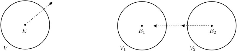
FIGURE 1. Consequences of a zero energy flux. Left: consider a particle with energy E enclosed by a volume V. If the particle can move, it could leave V and energy inside V is not conserved unless E = 0. If the particle cannot move, then there can be a non-zero rest energy E₀ which stays inside V. Particle decay of a particle with non-zero rest energy can also not happen. Right: interactions are possible, but only between particles of zero and non-zero energy, or between particles with zero energy. In this figure, particle 2 is attracted to particle 1, but to be consistent with zero-energy flux through V₂, it must have vanishing energy E₂ = 0. When it enters V₁, the total energy inside V₁ is then still conserved. Particle 1 is all the time at rest with rest energy E₁. Under Carroll boosts, energies stay the same, but velocities are rescaled.

2.2 Carroll Transformations From Lorentz Transformations

In this subsection, we derive the Carroll transformations from the Lorentz transformations by taking the limit of vanishing speed of light. We denote the Lorentz boost transformation parameter by $\vec{\beta }$ with $0\le |\vec{\beta }|<1$ and under a Lorentz boost we have

$c{t}^{\prime }={\gamma }_{\beta }\left(ct-\vec{\beta }\cdot \vec{x}\right),{\vec{x}}_{\parallel }^{{}^{\prime }}={\gamma }_{\beta }\left({\vec{x}}_{\parallel }-\vec{\beta }ct\right),{\vec{x}}_{\perp }^{{}^{\prime }}={\vec{x}}_{\perp },{\gamma }_{\beta }=\frac{1}{\sqrt{1-{\vec{\beta }}^2}},(10)$

with $\vec{x}={\vec{x}}_{\parallel }+{\vec{x}}_{\perp }$ the decomposition into components parallel and perpendicular to the boost parameter $\vec{\beta }$. To get the Carroll transformations from this, we consider the scaling limit (following [8])

$\vec{\beta }\equiv c\vec{b},c\to ϵc,ϵ\to 0.(11)$

The parameter $\vec{b}$ becomes the Carroll boost parameter, and its norm runs from zero to infinity. We keep it fixed in the limit ϵ → 0, and get

$t^{\prime }=t-\vec{b}\cdot \vec{x},{\vec{x}}^{{}^{\prime }}=\vec{x}.(12)$

These are the Carroll boosts. Under two consecutive Carroll boosts with parameters ${\vec{b}}_1$ and ${\vec{b}}_2$, we generate another one with boost parameter ${\vec{b}}_3={\vec{b}}_1+{\vec{b}}_2$. Notice the difference with the non-relativistic Galilei limit which is obtained by setting $\vec{\beta }=c^{-1}\vec{b}$ and then sending c → ∞. This gives the Galilei algebra as one can easily check. In a Galilei Universe, time is absolute, whereas in a Carroll Universe, space is absolute. Since the Lorentz boost factor γ_β → 1 in the Carroll limit, there is no Lorentz length contraction. There is no time dilation in a Carroll spacetime, but there is a time shift for events that are spatially separated. If a Carroll observer measures a time difference Δt between two events separated by $\mathrm{\Delta }\vec{x}$, then a boosted Carroll observer measures the same distance, but a shifted time difference given by

$\mathrm{\Delta }{t}^{\prime }=\mathrm{\Delta }t-\vec{b}\cdot \mathrm{\Delta }\vec{x}.(13)$

In other words, in a Carroll world time is relative, in contrast to the Galilean case, where space is relative. If a particle travels over a distance $\mathrm{\Delta }\vec{x}$ in a time Δt, then after a boost with $\vec{b}\cdot \vec{v}>1$ with $\vec{v}=\mathrm{\Delta }\vec{x}/\mathrm{\Delta }t$, we get Δt′ < 0. What this all really means is that the coordinate time is not a good clock to describe the motion of a particle. Instead we will in the next section introduce a proper time, the affine parameter along the worldline of the particle. This proper time serves as an evolution parameter describing the motion of a particle.

Since we can have Δt > 0 and Δt′ < 0, two Carroll observers do not necessarily agree on which event happened first. This sounds like a violation of causality, but it is not because for it to be a violation of causality physical information would have to be sent from one event to the other and since they are outside each other’s Carroll light cone (as a result of the physical separation and the fact that light cones are lines at a fixed point in space) this would require a particle with a nonzero velocity. In a Carroll Universe the latter is tantamount to a tachyonic particle. We will show further below that such particles exist and they in principle can lead to a violation of causality.

Spacetime distances become spatial distances in the c → 0 limit. The Minkowski metric degenerates as $\mathrm{d}{s}^2=-c^2\mathrm{d}{t}^2+\mathrm{d}{\vec{x}}^2\to \mathrm{d}{\vec{x}}^2$. Spatial distances are invariant under the Carroll group. Notice also that the Lorentz invariant $-c^2{t}^2+{\vec{x}}^2$ becomes the Carroll invariant ${\vec{x}}^2$ in the limit. Lightrays, for which this invariant is zero, in Carroll spacetime become $\vec{x}=0$ and t arbitrary. Therefore, the coordinate t parametrises the light cone. If $\vec{x}=0$, this means that light is not moving in space and the light cone has closed up.

Now we consider the contraction for the Lorentz transformations on energy and momentum

${\vec{p}}_{\parallel }^{\prime }={\gamma }_{\beta }\left({\vec{p}}_{\parallel }-\vec{\beta }\frac{E}{c}\right),{\vec{p}}_{\perp }^{\prime }={\vec{p}}_{\perp },\frac{E^{\prime }}{c}={\gamma }_{\beta }\left(\frac{E}{c}-\vec{\beta }\cdot \vec{p}\right),(14)$

with $\vec{p}={\vec{p}}_{\parallel }+{\vec{p}}_{\perp }$. In the Carroll limit we get

${\vec{p}}^{\prime }=\vec{p}-\vec{b}E,E^{\prime }=E.(15)$

These are indeed the correct transformation rules in Carroll spacetime (as dictated by the Carroll algebra), and we have rederived that the Hamiltonian is Carroll boost invariant.

We can also look at the velocity of a particle, $\vec{u}\equiv \mathrm{d}\vec{x}/\mathrm{d}t$. Under Lorentz boosts, the parallel and perpendicular components transform as

${\vec{u}}_{\parallel }^{\prime }\left(t^{\prime }\right)=\frac{{\vec{u}}_{\parallel }-\vec{\beta }c}{\left(1-\frac{\vec{\beta }\cdot \vec{u}}{c}\right)},{\vec{u}}_{\perp }^{\prime }\left(t^{\prime }\right)=\frac{{\vec{u}}_{\perp }\left(t\right)}{{\gamma }_{\beta }\left(1-\frac{\vec{\beta }\cdot \vec{u}}{c}\right)}.(16)$

Taking the limit of (Eq. 16) yields

${\vec{u}}^{\prime }\left(t^{\prime }\right)=\frac{\vec{u}\left(t\right)}{\left(1-\vec{b}\cdot \vec{u}\right)},(17)$

which was also obtained directly in Carroll spacetime, see (4). As we mentioned there, the transformation law of velocity is quite strange. If the velocity was zero, it remains zero after a (finite) Carroll boost. These are the particles, considered e.g. in [7]. If it was non-zero, we can boost it to any other value, as large as we want. Hence we have two distinct classes, not related by Carroll boosts: particles with zero velocity and particles with non-zero velocity. We can even change the direction of the velocity vector under a large enough Carroll boost. That is by itself not surprising, but for small enough boost parameters with $\vec{b}\cdot \vec{v}<1$, this will not happen.

Particles with non-zero velocity in the Carroll limit, satisfy v > c → 0, and hence they are tachyonic. As discussed above, they can cause violation of causality. Clearly this is unphysical. The strict c = 0 limit is unphysical. But this is not so different from the opposite limit, c → ∞. The strict c = ∞ limit is an unphysical theory as well, as it causes action at a distance. It nevertheless is useful to study the symmetries and dynamics that emerge in this limit. The proper way of thinking about both Carrollian and Galilei limits is to consider them as expansions in c/v and v/c respectively. We will discuss in more detail the dynamics of Carroll particles in the next section.

2.3 Representations of the Carroll Algebra

We will next discuss representations of the Carroll algebra in analogy with the massive and massless representations of the Poincaré algebra that are characterised by the eigenvalues of the momentum squared and the norm of the Pauli–Lubanski vector. Our results agree with those of [35].

The Carroll algebra consists of the generators H (Hamiltonian), P_i (spatial momenta), C_i (Carroll boosts), and J_ij = − J_ji (spatial rotations). The nonzero commutators are given by

$\begin{array}{ccc}\hfill & \hfill & \left[P_i,C_j\right]={\delta }_{ij}H,\hfill \end{array}(18)$

$\begin{array}{ccc}\hfill & \hfill & \left[J_{ij},P_k\right]={\delta }_{ik}{P}_j-{\delta }_{jk}{P}_i,\hfill \end{array}(19)$

$\begin{array}{ccc}\hfill & \hfill & \left[J_{ij},C_k\right]={\delta }_{ik}{C}_j-{\delta }_{jk}{C}_i,\hfill \end{array}(20)$

$\begin{array}{ccc}\hfill & \hfill & \left[J_{ij},J_{kl}\right]={\delta }_{ik}{J}_{jl}-{\delta }_{jk}{J}_{il}+{\delta }_{jl}{J}_{ik}-{\delta }_{il}{J}_{jk},\hfill \end{array}(21)$

where i, j, k, l run over 1, …, d. Representations are labelled by the eigenvalues of the central element H and the quartic Casimir $M^2=\frac{1}{2}{M}_{ij}{M}_{ij}$ where

$M_{ij}=H{J}_{ij}+C_i{P}_j-C_j{P}_i.(22)$

We will momentarily specialize to d = 3 and be quite explicit. Before doing so, we can describe the representations for general d a bit more heuristically. There are basically two cases, H = 0 and H ≠ 0. When H = 0, P and C commute and so they can be simultaneously diagonalized and states can be labeled by their eigenvalues. Rotations act on these eigenvalues and, possibly, simultaneously on an internal vector space. Once we extract an irreducible representation of the rotation algebra we can construct an irreducible representation of the Carroll algebra. In the absence of the internal vector space the zero energy irreducible representations can be labeled by P_iP_i, P_iC_i, and C_iC_i.

For H ≠ 0 the commutation relations of P_i and C_i are just like those of coordinates and momentum and can be represented by wave functions of P_i or equivalently C_i. We can combine these wave functions with a representation V of the rotation group, and then the rotation group acts simultaneously on this representation and by rotating P_i and C_i. States in the irreducible representation take the form |P_i⟩ ⊗ |ψ⟩ with $\left|\psi \right.⟩\in V$.

We now describe the case of d = 3 spatial dimensions more explicitly. For further details we refer to Supplementary Appendix SA. Here we summarise the main points.

For d = 3 it is useful to define W_k and S_k via

$M_{ij}={\epsilon }_{ijk}{W}_k,J_{ij}={\epsilon }_{ijk}{S}_k,(23)$

where ɛ_ijk is the Levi-Civita symbol. In d = 3 we can also define the operator L = S_iP_i (which is closely related to the helicity operator). The Carroll algebra is a semi-direct sum of the Abelian ideal spanned by {H, P_i} and the Euclidean algebra $\mathfrak{i}\mathfrak{s}\mathfrak{o}(d)$ spanned by {J_ij, C_i}, so one can consider induced representations using the little group method. Our findings are:

• When E ≠ 0 we can always go to a frame where p_i = 0 by performing a Carroll boost. In this case the little group is SO(3) and the eigenvalues of W_iW_i are E²s(s + 1) with s = 0, 1/2, 1, …. We can always go to a frame in which the states are of the form $|E\ne 0,\vec{p}=0,s,m\rangle$ where m = − s, − s + 1, …, s is the eigenvalue of S₃, the spin along the z-axis.

• When E = 0 the momentum p_i is Carroll boost invariant. Using a rotation we can without loss of generality set $\vec{p}=p{\widehat{e}}_3$ where ${\widehat{e}}_3$ is the unit vector along the z-axis. On such states W_i = ɛ_ijkC_jP_k so that W₃ = 0. The little group is ISO(2) and is generated by W₁, W₂, L. This case splits into two subcases. One for which W_iW_i = 0 and one for which W_iW_i > 0. We will always only consider the former. When W_iW_i = 0 we can always go to a frame in which the states are of the form $|E=0,\vec{p}=p{\widehat{e}}_3,\lambda \rangle$ where the helicity λ is the eigenvalue of S₃.

Further below we will see examples of either of these two representations.

2.4 Carroll Limit of de Sitter Space

In gravity, spacetime is curved, so it is important to study the Carroll limit of Lorentzian metrics. For the purposes of this paper, we look at one particular example relevant for cosmology, namely de Sitter space consisting of pure dark energy. The exponentially expanding Universe is described by the de Sitter metric, which in planar coordinates takes the form

$\mathrm{d}{s}^2=-c^2\mathrm{d}{t}^2+e^{2Ht}\mathrm{d}{\vec{x}}^2,(24)$

with H the Hubble constant and with isometry group SO(4, 1) in four spacetime dimensions. The isometry group contains three rotations and three spatial translations, and furthermore the isometries corresponding to scale and special conformal transformations which infinitesimally take the form

$\begin{array}{ccc}\hfill \delta t=-\frac{\alpha }{H},& \hfill & \delta \vec{x}=\alpha \vec{x},\hfill \end{array}(25)$

$\begin{array}{ccc}\hfill \delta t=-\frac{\vec{b}\cdot \vec{x}}{H},& \hfill & \delta \vec{x}=\left(\vec{b}\cdot \vec{x}\right)\vec{x}+\frac{\vec{b}}{2}\left(\frac{c^2}{H^2}{e}^{-2Ht}-{\vec{x}}^2\right).\hfill \end{array}(26)$

All factors of c are made explicit here, and so in the limit c → 0, keeping H fixed, the b-isometry becomes the Carroll isometry

${\delta }_{C}t=-\frac{\vec{b}\cdot \vec{x}}{H},{\delta }_C\vec{x}=\left(\vec{b}\cdot \vec{x}\right)\vec{x}-\frac{\vec{b}}{2}{\vec{x}}^2,(27)$

leaving the Carroll metric⁴ $\mathrm{d}{s}^2=e^{2Ht}\mathrm{d}{\vec{x}}^2$ invariant.⁵ In fact, this isometry is the infinitesimal special conformal transformation on ${\mathbb{R}}^3$, and the complete isometry group of this Carroll metric is the conformal group on ${\mathbb{R}}^3$. This hints towards a holographic description of (3 + 1)-dimensional de Sitter cosmology in terms of a three-dimensional Euclidean conformal field theory [38, 39] (see also [40, 41]), and generalizes straightforwardly to other dimensions. We obtained it here in the limit c → 0, but one finds the same conformal transformations at late times, t → ∞. This suggests that late time de Sitter cosmology is governed by Euclidean conformal correlators, and this conformal symmetry can be understood from the Carroll symmetry that is present at super-Hubble scales.

The metric in (Eq. 24) is written in planar coordinates and they fit into the FLRW ansatz. One can also use conformal time, τ = − 1/(aH), then we obtain the Carroll metric

$\mathrm{d}{s}^2=\frac{-c^2\mathrm{d}{\tau }^2+\mathrm{d}{\vec{x}}^2}{H^2{\tau }^2}\stackrel{c\to 0}{\to }\frac{1}{H^2{\tau }^2}\mathrm{d}{\vec{x}}^2,(28)$

which is again the metric on three-dimensional Euclidean space, up to a conformal factor.

3 Carroll Particles

In this section we consider various aspects of Carroll particles. Point particles can conveniently be described in an extended phase space system, which is useful for Carroll particles (see e.g. also [7]) as generic Carroll systems do not seem to have a well-defined initial value problem with respect to coordinate time. This follows from the fact that, as discussed in the previous section, Carroll transformations can change the direction of trajectories and even make them frozen in time. To have a well-defined initial value problem one can employ particles which use some internal clock time (cf. proper time) which can be used to define dynamics.

3.1 Extended Phase Space

We first briefly recap how the extended phase space formulation works for ordinary particles. Consider the worldline action for a particle given by

$S_0=-\int \text{d}s(E\cdot \dot{t}-\vec{p}\cdot \dot{\stackrel{⃗}{x}}),(29)$

which describes an extended phase space with d + 1 coordinates and d + 1 momenta (d equals the number of spatial coordinates) and zero Hamiltonian. Notice that the combination $E\cdot \dot{t}-\vec{p}\cdot \dot{\stackrel{⃗}{x}}$ is invariant under both Lorentz and Carroll boosts.

To reproduce some familiar systems from this we consider the class of actions

$S=-\int \text{d}s(E\cdot \dot{t}-\vec{p}\cdot \dot{\stackrel{⃗}{x}}-{\lambda }_{\alpha }{O}_{\alpha }+H),(30)$

where O_α are some constraints with Lagrange multipliers λ_α and H is some Hamiltonian on the extended phase space. In order for this to make sense we need that {H, O_α} = c_αβO_β so that time evolution preserves the constraint surface. We can have first class (commuting on the constraint surface) or second class constraints. In the first case the Lagrange multipliers will not be fixed as a reflection of the gauge symmetry which first class constraints typically generate. In the second case the Lagrange multipliers will typically be fixed by the constraints and the equations of motion, and we can pass to the reduced phase space. One way to find the actual dynamics of the system, is by examining the resulting field equations.

If the system has a set of symmetry generators on the extended phase space, the constraints and Hamiltonian must be compatible with these symmetries in order to preserve them. This can be studied canonically (i.e. through Poisson brackets of O_α and H with the symmetry generators) but also through the action (i.e. verifying that it is invariant under these symmetries). Now, let us consider some cases:

1) O₁ = E − p²/2m, H = 0. This includes a first class constraint. The field equations are

$\dot{t}={\lambda }_1,\dot{E}=0,\dot{\stackrel{⃗}{p}}=0,\dot{\stackrel{⃗}{x}}=\frac{{\lambda }_1}{m}\vec{p},(31)$

and one sees that these still depend on λ₁. The action is s-reparametrization invariant, where one also needs to transform λ₁. We can eliminate λ₁ to obtain $\mathrm{d}E/\mathrm{d}t=\mathrm{d}\vec{p}/\mathrm{d}t=0$ and $\vec{p}=m\mathrm{d}\vec{x}/\mathrm{d}t$ where everything depends on t rather than s. Moreover E = p²/2m. This describes a standard free massive non-relativistic particle. Eliminating the constraints in the action gives the usual form

$S=\int \text{d}t\frac{p^2}{2m}=\frac{m}{2}\int \text{d}t{\dot{\stackrel{⃗}{x}}}^2,(32)$

where the dot in the last equation now stands for the derivative with respect to t.

2) O₁ = E − p²/2m, O₂ = t − s; H = 0. We now have second class constraints and the field equations are

$\dot{t}={\lambda }_1,\dot{E}=-{\lambda }_2,\dot{\stackrel{⃗}{p}}=0,\dot{\stackrel{⃗}{x}}=\frac{{\lambda }_1}{m}\vec{p}.(33)$

If we combine these with the constraints we find λ₂ = 0 and λ₁ = 1, so the Lagrange multipliers are completely fixed. Again, one finds a standard non-relativistic particle, since the extra constraint simply relates t to s but does not have any essential impact.

3) O₁ = E, H = p²/2m. This includes a first class constraint plus a non-trivial Hamiltonian. The field equations are

$\dot{t}={\lambda }_1,\dot{E}=0,\dot{p}=0,\dot{\stackrel{⃗}{x}}=\vec{p}/m,(34)$

which is once more a standard particle. However, t is no longer the usual time variable, as this role has been taken over by s. In fact the dynamics in t and E completely decouples. The energy is not given by E but by the Hamiltonian H.

4) $O_1=E-\mathcal{H}(p,x),H=0$. This is a another first class constraint and case 1 above is a special case of this. Rather than looking at the field equations, we integrate out E and λ₁ which yields $\dot{t}={\lambda }_1$ and $E=\mathcal{H}(p)$. Plugging this into the action we obtain

$S=\int \text{d}t\left(\vec{p}\cdot \frac{\text{d}\vec{x}}{\text{d}t}-\mathcal{H}(p,x)\right),(35)$

which is just the Lagrangian in first order form. So such a first class constraint corresponds to standard dynamics in general.

3.2 Carroll Symmetry and Single Carroll Particles

We now apply the extended phase space technique to the dynamics of Carroll particles, starting with a single particle. The standard Carroll algebra has generators

$E,E{x}_i,p_j,x_{[i}{p}_{j]},i,j=1,\dots ,d,(36)$

for time translations, Carroll boosts, space translations and rotations respectively. It follows again that E commutes with the other generators, and hence is a central charge. One could imagine more complicated realizations of this algebra on a given phase space, but we will restrict to this simple choice.

To add a constraint consistent with Carroll symmetry, it must Poisson commute with these generators. Because of time and space translational invariance (or Poisson commutability with E and $\vec{p}$) the constraint can only depend on E and $\vec{p}$, and rotational invariance restricts it to a function of E and p². But this can only commute with the generators $E\vec{x}$ if it does not depend on p². It follows that E − E₀ is the only constraint that we can introduce. This produces the rather trivial case of a particle with energy E₀ and unconstrained momenta, which is also seen in the representation theory in section 2.3. The extended phase space action based on this constraints reads

$S=-\int \mathrm{d}s\left(E\cdot \dot{t}-\vec{p}\cdot \dot{\stackrel{⃗}{x}}-\lambda \left(E-E_0\right)\right),(37)$

giving rise to the equations of motion

$\dot{t}=\lambda ,\dot{E}=0,\dot{\stackrel{⃗}{x}}=0,\dot{\stackrel{⃗}{p}}=0.(38)$

This corresponds to the Carroll particle at rest. It has zero velocity and constant energy E₀. This is to be expected since in the Carroll limit, the light-cone closes and only particles with zero velocity can survive the c → 0 limit.

There is, however, an interesting alternative choice corresponding to the introduction of two constraints, E = 0 and $p^2=p_0^2$. This is consistent because the commutator of the constraint $p^2-p_0^2$ with $E\vec{x}$ is proportional to the first constraint. This possibility was not included in the phase space analysis of [7]. It is easy to write down an action for this case. Using the extended phase space action (30) with constraints $O_1=E,O_2=p^2-p_0^2$ and H = 0 for some constant p₀. One can subsequently eliminate the Lagrange multipliers to get ${\lambda }_1=\dot{t}$ and

${\lambda }_2=-\frac{1}{2p_0}\sqrt{{\dot{\stackrel{⃗}{x}}}^2},(39)$

such that the action becomes

$S\left[\vec{x}\right]=p_0\int \mathrm{d}s\sqrt{\dot{\stackrel{⃗}{x}}\cdot \dot{\stackrel{⃗}{x}}},L\left(\vec{x},\dot{\stackrel{⃗}{x}}\right)=p_0\sqrt{\dot{\stackrel{⃗}{x}}\cdot \dot{\stackrel{⃗}{x}}}.(40)$

Indeed, from the Lagrangian follows the momentum

$\vec{p}=\frac{\partial L}{\partial \dot{\stackrel{⃗}{x}}}=p_0\frac{\dot{\stackrel{⃗}{x}}}{\sqrt{{\dot{\stackrel{⃗}{x}}}^2}}=p_0\vec{n},(41)$

which satisfies the contraint

$O_2\equiv {\vec{p}}^2-p_0^2=0,(42)$

as it should. The equation of motion says that $\vec{p}$ and therefore $\vec{n}$ is constant in time. E and t decouple from the dynamics and there is still reparametrization symmetry on the worldline. One can use this to fix a gauge $|\dot{\stackrel{⃗}{x}}|=p_0$. Then the particle trajectories are of the form $\vec{x}(s)={\vec{p}}_{0}s+{\vec{x}}_0$ for some vector ${\vec{p}}_0$ with $|{\vec{p}}_0|=p_0$. The solution for the momentum then becomes $\vec{p}={\vec{p}}_0$, and we recall that the energy is zero.

We thus confirm the properties concluded in the previous section as a consequence of having a zero energy flux: If particles can move, they must have zero energy, and if they have non-zero energy, they cannot move and there is only rest energy. Having established this, we now turn to the question of how these particles can arise from a relativistic theory by taking the limit c → 0.

3.3 Carroll Particles From Relativistic Particles

Let us consider a free relativistic particle with energy E, mass m and momentum $\vec{p}$. We denote the velocity of the particle by $\vec{u}=\mathrm{d}\vec{x}/\mathrm{d}t$ and $u^2=\vec{u}\cdot \vec{u}$. The relations between them are given by

$\vec{p}=\frac{m\vec{u}}{\sqrt{1-\frac{u^2}{c^2}}},E=\frac{m{c}^2}{\sqrt{1-\frac{u^2}{c^2}}},E^2={\vec{p}}^2{c}^2+m^2{c}^4,(43)$

and hold in any Lorentz frame.

We now encounter a subtlety when taking the Carroll limit. The gamma-factor associated with the particle with velocity $\vec{u}$ does not seem to have a well-defined limit

${\gamma }_u=\frac{1}{\sqrt{1-\frac{u^2}{c^2}}}\underrightarrow{c\to 0}?(44)$

Notice that this is a different object compared with the gamma-factor in the Lorentz transformation that contains the boost parameter $\vec{\beta }$, which always goes to unity in the Carroll limit: γ_β → 1. Here we are not contracting the boost parameter, instead we are searching for a consistent limit of physical quantities under a Carroll contraction.

If we keep u fixed and non-zero, this expression becomes imaginary in the Carroll limit. It seems there are two options: either we require that the Carroll velocity identically vanishes, u = 0, and then γ_u → 1, or we allow for imaginary values

${\gamma }_u\to \mp i\frac{c}{u},u\equiv |\vec{u}|,(45)$

where we allow for the two branches of the square root. This expression for γ_u vanishes in the strict Carroll limit, but this is the leading term in the small c expansion.

The case of zero velocity, $\vec{u}=0$ corresponds to the Carroll particle at rest. The limit c → 0 is rather trivial, but we take the limit such that there is still rest energy E₀. To achieve this we keep the combination mc² fixed in the Carroll limit. The energy and momenta for these particles then are

$E=E_0=m{c}^2,\vec{p}=0.(46)$

We now consider the more interesting case in which ${\gamma }_u=\mp i\frac{c}{u}$. Substituting this into the expression for the momentum, we find

$\vec{p}=\mp \left(imc\right)\frac{\vec{u}}{u}=\mp \left(imc\right)\vec{n}.(47)$

This can only make sense and yield real and non-zero values of the momentum if we keep mc fixed and the original relativistic particle was a tachyon, so

$p_0\equiv -imc,(48)$

for some real p₀ and therefore m² < 0. That tachyons enter into the picture is not so surprising since (45) also follows from u² > c². Notice furthermore that the scaling law on the mass m is different as compared to the case of the relativistic massive particle with zero velocity, where the mass m scales like ϵ⁻² in the Carroll limit. The momentum of these tachyon-like particles satisfies the constraint $p^2=p_0^2$ since $\vec{n}$ is of unit norm. Furthermore, we find that the Carroll particle has zero energy because of the cancellation ${\vec{p}}^2{c}^2+m^2{c}^4={\vec{p}}^2{c}^2-p_0^2{c}^2=0$ (thanks to the tachyon!), and hence the energy and momenta for these particles are

$E=0,\vec{p}=\pm p_0\vec{n}.(49)$

Notice the ± sign in the momentum, which is a consequence of the fact that the momentum as a function of the velocity is no longer single-valued (as follows from (Eq. 45)). The velocity u is undetermined and arbitrary but non-vanishing. These Carroll particles, for p₀ ≠ 0, cannot be put to rest by a boost, they always move.

It is interesting to contrast Eq. 49 with (Eq. 41). The latter does not have a sign ambiguity. To go from (41–49) we need to divide the numerator and the denominator of (Eq. 41) by $\dot{t}$. However $\dot{t}$ can have either sign which is the origin of the sign ambiguity of $\vec{p}$ when expressed in terms of the velocity $\vec{u}=\dot{\stackrel{⃗}{x}}/\dot{t}$. This illustrates what was stated previously, namely that the more convenient evolution parameter is the proper time s as opposed to coordinate time t.

A similar representation with zero energy can be found from the Carroll limit of massless particles. These have dispersion relation E = pc, and for fixed p, we have E → 0 in the Carroll limit.

3.4 Many-Particle Carroll Systems

It is relatively easy to generalize the extended phase space approach to many particles which we label by a = 1, …, N. The action on extended phase space is now

$S=-\int ds\left(E_a{\dot{t}}_a-{\vec{p}}_a\cdot {\dot{\stackrel{⃗}{x}}}_a-{\lambda }_{\alpha }{O}_{\alpha }+H\right),(50)$

where we sum over a (the number of particles) and α (the number of constraints). To get a standard classical mechanical system of many particles, we can either choose a set of first class constraints $E_a-\mathcal{H}({\vec{x}}_a,{\vec{p}}_a)=0$ for all a with $\mathcal{H}$ the total Hamiltonian (that we assume to be time independent) and H = 0, or choose first class constraints E_a = 0 and add an explicit Hamiltonian H just as we did for the single particle case. In either case, using the gauge symmetries, this leads to standard actions for multiple particles with a single time variable $t={\sum }_{a=1}^N{t}_a$.

We now apply this to a system of many Carroll particles, as was also considered in Ref. [7]. In the case of N particles, and can realise the generators of the Carroll algebra as

$\sum _a{E}_a,\sum _a{E}_a{\vec{x}}_a,\sum _a{\vec{p}}_a,\sum _a{x}_a^{\left[k\right.}{p}_a^{\left.l\right]},a=1,\dots ,N.(51)$

Apart from rotations, the following set of building blocks commute with the Carroll algebra:

$E_a,{\vec{x}}_a-{\vec{x}}_b,E_a{\vec{p}}_b-E_b{\vec{p}}_a,(52)$

but also the combinations

$E_a{t}_{bc}-{\vec{p}}_a\cdot {\vec{x}}_{bc},(53)$

with t_ab = t_a − t_b and ${\vec{x}}_{ab}={\vec{x}}_a-{\vec{x}}_b$. The building blocks (52) and (53) form a closed algebra under the Poisson bracket⁶ and are thus first class.

To construct an interacting Carroll system, we need to find a set of commuting constraints, or as shown above, a set of commuting constraints plus a Hamiltonian. In fact, we only need that the variation of the Hamiltonian and the constraints is proportional to the constraints, as in that case we can make the theory invariant by letting the Lagrange multipliers transform.

For Carroll symmetry this means that we can take first class constraints of the form E_a − H where H is now some rotationally invariant function of the invariants (52). Any H which is a function of (Eq. 52), and rotationally invariant, can in principle be used, giving rise to a fairly rich spectrum of possible interacting Carroll particles. This does not contradict the representation theory as that only applies to the center of mass degree of freedom. These examples were studied in [7].

It is also possible to take the other point of view where we for example impose first class constraints E_a = 0 for all a and add an explicit Hamiltonian H. But now something interesting happens. As long as the Hamiltonian does not involve the time coordinates, its Poisson bracket with the generator of Carroll boosts will be proportional to a linear combination of the E_a. This is not zero, but we can compensate for this by a suitable transformation rule for the Lagrange multipliers. Therefore, we need not worry about boost invariance of H, and in fact any H which preserves translations and rotations is admissible. This is no different from standard many-particle dynamics. It looks like any many-particle Hamiltonian can be dressed with a Carroll symmetric center of mass degree of freedom to provide a Carroll invariant system of particles each with zero energy. This case was not considered in [7], and it might be instructive to get these systems directly as a c → 0 limit of a relativistic many-particle system.

4 Carroll Field Theory

In this section, we switch to field theory, and prepare for the application to cosmology we have in mind. The starting point is to construct Lagrangians that are Carroll invariant and can be obtained from a c → 0 limit of a relativistic theory or through an expansion in small c. We treat here the real scalar field and the Maxwell field as examples.

4.1 Scalar Field

Consider a relativistic real scalar field ϕ. Under a Lorentz boost, it transforms as

$\delta \varphi =ct\vec{\beta }\cdot \vec{\partial }\varphi +\frac{1}{c}\vec{\beta }\cdot \vec{x}{\partial }_t\varphi .(54)$

The relativistic scalar field lagrangian density

$\mathcal{L}=\frac{1}{2c^2}{\left({\partial }_t\varphi \right)}^2-\frac{1}{2}{\left({\partial }_i\varphi \right)}^2-V\left(\varphi \right).(55)$

transforms into a total derivative, as is well known. The conjugate momentum is

${\pi }_{\varphi }=\frac{1}{c^2}{\partial }_t\varphi .(56)$

The relativistic energy-momentum tensor is

${T^{\mu }}_{\nu }={{\delta }^{\mu }}_{\nu }\left(-\frac{1}{2}{\partial }_{\rho }\varphi {\partial }^{\rho }\varphi -V\left(\varphi \right)\right)+{\partial }^{\mu }\varphi {\partial }_{\nu }\varphi ,(57)$

and is symmetric when raising the indices.

For a quadratic potential of the form $V(\varphi )=\frac{1}{2}\frac{m^2{c}^2}{{\hslash }^2}{\varphi }^2$ (in SI units), we get the usual relativistic dispersion relation from a plane wave ansatz $\varphi \propto e^{i\vec{k}\cdot \vec{x}+i\omega t}$,

$E^2\equiv {\hslash }^2{\omega }^2=c^2{\vec{p}}^2+m^2{c}^4,(58)$

with $\vec{p}=\hslash \vec{k}$.

We now make an expansion around c = 0 so we write⁷

$\varphi =c^{\mathrm{\Delta }}\left({\varphi }_0+c^2{\varphi }_1+c^4{\varphi }_2+\cdots \right)=c^{\mathrm{\Delta }}\sum _{n=0}^{\infty }{\varphi }_n{c}^{2n},(59)$

for some Δ. Defining as before $\vec{\beta }=c\vec{b}$, with $\vec{b}$ the Carroll boost parameter, one finds the Carroll transformations⁸, for n > 0,

$\delta {\varphi }_0=\vec{b}\cdot \vec{x}{\partial }_t{\varphi }_0,\delta {\varphi }_n=\vec{b}\cdot \vec{x}{\partial }_t{\varphi }_n+t\vec{b}\cdot \vec{\partial }{\varphi }_{n-1}.(60)$

The field ϕ₀ is a scalar field with respect to Carroll transformations, as the Carroll generator for boosts is C_i = xⁱ∂_t. The higher order modes in the expansion are not Carroll scalars, and transform into each other under boosts.

Using this expansion, it is rather straightforward to construct Carroll invariant Lagrangians. For free fields, we find, for the two lowest orders in the small-c expansion,

${\mathcal{L}}_0=\frac{1}{2}{\dot{\varphi }}_0^2,{\mathcal{L}}_1={\dot{\varphi }}_0{\dot{\varphi }}_1-\frac{1}{2}{\partial }_i{\varphi }_0{\partial }_i{\varphi }_0,(61)$

where we defined ${\mathcal{L}}_0$ and ${\mathcal{L}}_1$ via $\mathcal{L}=c^{2\mathrm{\Delta }-2}\left({\mathcal{L}}_0+c^2{\mathcal{L}}_1+O(c^4)\right)$. One can explicitly check that both ${\mathcal{L}}_0$ and ${\mathcal{L}}_1$ transform into total derivatives so their corresponding actions are invariant with the appropriate boundary conditions. Note that ${\mathcal{L}}_1$ contains the field ϕ₁ which does not transform as a scalar field under Carroll transformations. As we discuss in more detail below ${\mathcal{L}}_1$ is not Carroll boost invariant but can be made to be by adding a Lagrange multiplier that sets ${\dot{\varphi }}_0$ equal to zero on shell.

It is easy to add interactions, starting from a Lorentz invariant potential by simply substituting the expansion 59) in the potential. Different choices can be made however, depending on how the coupling constants in the potential scale with c. We consider here the simplest example of a quadratic potential. Assuming the parameters depend homogeneously on c there are still two choices, namely keeping E₀ ≡ mc² (or ω₀ = E/ℏ) fixed, or keeping the Compton wavelength λ⁻¹ = μ ≡ mc/ℏ fixed, similar to the analysis of the relativistic particle in Section 3.3.

For fixed ω₀, we get

$\begin{array}{ccc}\hfill {\mathcal{L}}_0& =\hfill & \frac{1}{2}{\dot{\varphi }}_0^2-\frac{1}{2}{\omega }_0^2{\varphi }_0^2,\hfill \\ \hfill {\mathcal{L}}_1& =\hfill & {\dot{\varphi }}_0{\dot{\varphi }}_1-\frac{1}{2}{\partial }_i{\varphi }_0{\partial }_i{\varphi }_0-{\omega }_0^2{\varphi }_0{\varphi }_1.\hfill \end{array}(62)$

The equation of motion associated to ${\mathcal{L}}_0$ is

${\ddot{\varphi }}_0+{\omega }_0^2{\varphi }_0=0.(63)$

For ${\mathcal{L}}_1$ the equation of motion for ϕ₁ is the same as in (Eq. 63)⁹, but we get a second equation by varying ϕ₀,

${\ddot{\varphi }}_1+{\omega }_0^2{\varphi }_1={\partial }^2{\varphi }_0.(64)$

The solutions to the response of ϕ₁ to ϕ₀ can be found in terms of plane waves,

${\varphi }_0=e^{i\vec{k}\cdot \vec{x}+i{\omega }_{0}t}+c.c.,{\varphi }_1=\frac{i}{2{\omega }_0}{\vec{k}}^{2}t{e}^{i\vec{k}\cdot \vec{x}+i{\omega }_{0}t}+c.c.(65)$

Both ϕ₀ and ϕ₁ are fields arising in the expansion around c = 0, and we can use them to reconstruct the relativistic scalar using (59): ϕ = ϕ₀ + c²ϕ₁ + ⋯ , where we put Δ = 0 for simplicity. Then the full relativistic plane wave solutions are known of course, and involve the frequency in (58). We can expand the relativistic dispersion relation around c = 0 using

$\omega ={\omega }_0+c^2\frac{{\vec{k}}^2}{2{\omega }_0}+\cdots ,e^{i\omega t}=e^{i{\omega }_{0}t}\left(1+i{c}^2\frac{{\vec{k}}^2}{2{\omega }_0}t+\cdots \right),(66)$

where we remind that ω₀ = mc²/ℏ which we kept fixed in the Carroll limit. One now sees that this expansion is reproducing the expansion in ϕ using (Eq. 65), as it should. Furthermore, if we perform an infinitesimal Carroll transformation on the right hand side of the dispersion relation, we find $\delta \omega =-c^2\vec{k}\cdot \vec{b}=-c\vec{k}\cdot \vec{\beta }$, which is the first term in the expression for an infinitesimal Lorentz transformation on the energy or frequency. If we keep expanding further in the ϕ_n, we will reconstruct the full relativistic solution.

Now we consider the second possibility, in which we keep μ = mc/ℏ fixed in the Carroll limit. Then we find

$\begin{array}{ccc}\hfill {\mathcal{L}}_0& =\hfill & \frac{1}{2}{\dot{\varphi }}_0^2,\hfill \\ \hfill {\mathcal{L}}_1& =\hfill & {\dot{\varphi }}_0{\dot{\varphi }}_1-\frac{1}{2}{\partial }_i{\varphi }_0{\partial }_i{\varphi }_0-\frac{1}{2}{\mu }^2{\varphi }_0^2.\hfill \end{array}(67)$

The equations of motion for ${\mathcal{L}}_0$ is

${\ddot{\varphi }}_0=0\Rightarrow {\varphi }_0=f\left(\vec{x}\right)+g\left(\vec{x}\right)t.(68)$

For ${\mathcal{L}}_1$ the equation of motion for ϕ₁ is the same as in (Eq. 68), but we get a second equation

${\ddot{\varphi }}_1={\partial }^2{\varphi }_0-{\mu }^2{\varphi }_0.(69)$

If ${\ddot{\varphi }}_1=0$, and upon taking plane spatial waves for ϕ₀ (i.e. $f(\vec{x})=e^{i\vec{k}\cdot \vec{x}}+c.c$.), one arrives at the tachyonic modes for a single particle again, with ${\vec{k}}^2+{\mu }^2=0$. However, the interaction between ϕ₀ and ϕ₁ provides non-trivial solutions with ${\vec{k}}^2+{\mu }^2>0$.

The relativistic dispersion relation in this case is written as $\omega =\pm c\sqrt{{\vec{k}}^2+{\mu }^2}$ and vanishes in the strict Carroll limit. This corresponds to Carroll representations with vanishing energy, E = 0. The first correction is linear in c and gives already the exact result for ω.

To conclude this part of the discussion, we find again, just as for the relativistic particle, two representations in the Carroll limit, those with non-zero energy E₀ = ℏω₀ = mc² and those with zero energy where we kept mc/ℏ fixed.

We now consider some further properties of ${\mathcal{L}}_0$ and ${\mathcal{L}}_1$.

4.1.1 Energy-Momentum Tensor

We start with the Carroll invariant Lagrangian

${\mathcal{L}}_0=\frac{1}{2}{\dot{\varphi }}_0^2-V\left({\varphi }_0\right).(70)$

The corresponding energy-momentum tensor is¹⁰,

$\begin{array}{cc}\hfill {T^t}_t& =-\left(\frac{1}{2}{\dot{\varphi }}_0^2+V\right),{T^i}_t=0,\hfill \\ \hfill {T^t}_i& =-{\dot{\varphi }}_0{\partial }_i{\varphi }_0,{T^i}_j=\left(\frac{1}{2}{\dot{\varphi }}_0^2-V\right){{\delta }^i}_j.\hfill \end{array}(72)$

This energy-momentum tensor obeys the Carroll transformation laws (Eq. 9) and the constraint that ${T^i}_t=0$. Notice that spatial derivatives ∂_iϕ are absent in ${\mathcal{L}}_0$ but they do appear in the energy-momentum tensor. Their appearance is important for showing that the energy-momentum tensor is conserved on shell. Notice furthermore that this energy-momentum tensor arises as the leading order term in the expansion

${T^{\mu }}_{\nu }=T_{\left(0\right)\nu }^{\mu }+c^2{T}_{\left(1\right)\nu }^{\mu }+\cdots ,(73)$

where the left-hand side stands for the relativistic energy-momentum tensor which transforms as a tensor under Lorentz transformations. On the right-hand side, the leading term ${T_{(0)}^{\mu }}_{\nu }$ transforms as a Carroll tensor and in particular it should obey ${T^i}_t=0$. The first order correction to it, T₍₁₎ does not transform as a tensor under the Carroll group (it will transform into T₍₀₎ as well), just like ϕ₁ does not transform as a scalar under Carroll boosts. Therefore T₍₁₎ is not expected to satisfy the Carroll identity ${T^i}_t=0$, as we will explicitly see below.

The theory described by the next-to-leading order action has the Lagrangian

${\mathcal{L}}_1={\dot{\varphi }}_0{\dot{\varphi }}_1-\frac{1}{2}{\partial }_i{\varphi }_0{\partial }_i{\varphi }_0,(74)$

where we ignored possible potential terms. Using (71), adapted to a theory containing two scalar fields, the energy-momentum tensor components now read

$\begin{array}{ccc}\hfill & \hfill & {T^t}_t=-{\dot{\varphi }}_0{\dot{\varphi }}_1-\frac{1}{2}{\left({\partial }_i{\varphi }_0\right)}^2,{T^i}_t={\dot{\varphi }}_0{\partial }_i{\varphi }_0,\hfill \\ \hfill & \hfill & {T^t}_i=-{\dot{\varphi }}_1{\partial }_i{\varphi }_0-{\dot{\varphi }}_0{\partial }_i{\varphi }_1,{T^i}_j={{\delta }^i}_j{\mathcal{L}}_1+{\partial }^i{\varphi }_0{\partial }_j{\varphi }_0.\hfill \end{array}(75)$

One can check that it is conserved, but it does not satisfy the Carroll constraint ${T^i}_t=0$, as explained above. One can also check that it follows from the relativistic symmetric energy-momentum tensor by expanding in powers of c, i.e. the $T_{(1)\nu }^{\mu }$ term in (Eq. 73).

The expansion of the relativistic scalar field Lagrangian around c = 0 leads to (after appropriately rescaling the Lagrangian with c^2−2Δ) the Lagrangians ${\mathcal{L}}_0$ and ${\mathcal{L}}_1$. The Lagrangian ${\mathcal{L}}_0$ is Carroll boost invariant while the Lagrangian ${\mathcal{L}}_1$ is not.¹¹ We can however modify ${\mathcal{L}}_1$ by adding a Lagrange multiplier to make it Carroll boost invariant. The Lagrange multiplier sets to zero ${\dot{\varphi }}_0$ (so that now ${\mathcal{L}}_1$ is the leading order Lagrangian in the expansion of the free scalar theory). This leads to

$\mathcal{L}={\dot{\varphi }}_0{\dot{\varphi }}_1-\frac{1}{2}{\partial }_i{\varphi }_0{\partial }_i{\varphi }_0+\tilde{\chi }{\dot{\varphi }}_0,(76)$

with Lagrange multiplier $\tilde{\chi }$. We can absorb ${\dot{\varphi }}_1$ into $\tilde{\chi }$ leading to

$\mathcal{L}=-\frac{1}{2}{\partial }_i{\varphi }_0{\partial }_i{\varphi }_0+\chi {\dot{\varphi }}_0,(77)$

where the new Lagrange multiplier is χ.

We can obtain the latter Lagrangian also directly by taking a Carroll limit. Let us consider the following relativistic Lagrangian density consisting of two scalar fields χ and ϕ:

$\mathcal{L}=-\frac{c^2}{2}{\chi }^2+\chi {\partial }_t\varphi -\frac{1}{2}{\left({\partial }_i\varphi \right)}^2-V\left(\varphi \right).(78)$

From the equation of motion for χ,

$\chi =\frac{1}{c^2}{\partial }_t\varphi ,(79)$

it is easy to see that the Lagrangian density in (Eq. 78) is engineered such that integrating out χ yields a canonical relativistic scalar field Lagrangian as given in (Eq. 55). And of course, χ is identical to the conjugated momentum when seen in first order formalism. It is however not a scalar field under Lorentz transformations.

In the Carroll limit c → 0 keeping both χ and ϕ fixed, we find that the Lagrangian density in (Eq. 78) becomes

$\mathcal{L}=\chi \dot{\varphi }-\frac{1}{2}{\left({\partial }_i\varphi \right)}^2-V\left(\varphi \right).(80)$

The action is invariant under Carroll boosts if we assign the transformation laws

$\delta \varphi =\vec{b}\cdot \vec{x}\dot{\varphi },\delta \chi =\vec{b}\cdot \vec{x}\dot{\chi }+\vec{b}\cdot \vec{\partial }\varphi .(81)$

The field equation of χ sets $\dot{\varphi }=0$, in fact χ is a Lagrange multiplier. This is consistent with the expression (79) and the fact that both χ and ϕ are kept fixed in the c → 0 limit. The situation is then as described in the introduction, and in the small c-expansion, this means that the scalar field should be slowly varying in time.

Notice that the Lagrangian (80) is actually very similar to (74). It seems that all one needs to do is to perform the field redefinition $\chi ={\dot{\varphi }}_1$. However this changes the Lagrangian in a non-trivial way as varying ϕ₁ does not lead to the same equation of motion as varying χ. Using the on-shell constraint $\dot{\varphi }=0$, the resulting energy-momentum tensor is now given by

$\begin{array}{cc}\hfill {T^t}_t=& -\left(V+\frac{1}{2}{\left({\partial }_i\varphi \right)}^2\right),{T^i}_t=0,\hfill \\ \hfill {T^t}_j=& -\chi {\partial }_j\varphi ,{T^i}_j=-\left(V+\frac{1}{2}{\left({\partial }_i\varphi \right)}^2\right){{\delta }^i}_j+{\partial }_i\varphi {\partial }_j\varphi .\hfill \end{array}(82)$

It is conserved on-shell and indeed, as required by Carroll symmetry, ${T^i}_t=0$. We see now that if we subject ${\mathcal{L}}_1$ in (Eq. 74) to ${\dot{\varphi }}_0=0$, that the two theories are equivalent when χ plays the role of ${\dot{\varphi }}_1$ and the energy-momentum tensor in (Eq. 74) becomes the same as (82).

4.2 Maxwell Theory

We can also consider Carrollian versions of Maxwell’s theory. In analogy to the scalar field theory case treated in the previous section, we present here again two perspectives. One in which we consider an expansion for slow speed of light and the other based on taking the c → 0 limit, as has been studied in e.g. [8–11, 43]. Furthermore, in parallel with similar investigations of the non-relativistic expansion/limit (c → ∞) of Maxwell theory (see e.g. [44, 45]), one finds two distinct sectors, the electric and the magnetic.

4.2.1 Expansions

The Maxwell field A_μ transforms under Lorentz boosts as

$\delta A_{\mu }=ct\vec{\beta }\cdot \vec{\partial }{A}_{\mu }+\frac{1}{c}\vec{\beta }\cdot \vec{x}{\partial }_t{A}_{\mu }+\bar{\delta }{A}_{\mu },(83)$

where $\bar{\delta }{A}_0=\vec{\beta }\cdot \vec{A}$ and $\bar{\delta }\vec{A}=\vec{\beta }{A}_0$. Here we have used the transformation δA_μ = ξ^ν∂_νA_μ + ∂_μξ^νA_ν under a general coordinate transformation and used its restriction to a Lorentz transformation via ${\xi }^0=\vec{\beta }\cdot \vec{x}/c$, ξⁱ = x⁰/cβⁱ = tβⁱ. From now on we will use A_t = cA₀, which allows¹² for an expansion in even powers of c such that

$A_t=c^{\mathrm{\Delta }}\left(A_t^{\left(0\right)}+c^2{A}_t^{\left(1\right)}+\cdots ,\right)=c^{\mathrm{\Delta }}\sum _{n=0}^{\infty }{A}_t^{\left(n\right)}{c}^{2n},(84)$

for some Δ, and likewise for A_i with the same Δ.

Again we define $\vec{\beta }=c\vec{b}$, with $\vec{b}$ the Carroll boost parameter. The fields in the expansion above then transform as

$\delta A_t^{\left(n\right)}=\vec{b}\cdot \vec{x}{\partial }_t{A}_t^{\left(n\right)}+t\vec{b}\cdot \vec{\partial }{A}_t^{\left(n-1\right)}+\vec{b}\cdot {\vec{A}}^{\left(n-1\right)},(85)$

$\delta A_i^{\left(n\right)}=\vec{b}\cdot \vec{x}{\partial }_t{A}_i^{\left(n\right)}+b_i{A}_t^{\left(n\right)}+t\vec{b}\cdot \vec{\partial }{A}_i^{\left(n-1\right)},(86)$

where the transformations for n = 0 are included using $A_{\mu }^{(-1)}\equiv 0$. The field $(A_t^{(0)},A_i^{(0)})$ is a vector field with respect to Carroll transformations. The higher order modes in the expansion transform into each other under boosts.

Next we study the expansion of the Maxwell Lagrangian

$\mathcal{L}=\frac{1}{2c^2}{\left(E^i\right)}^2-\frac{1}{4}{\left(F_{ij}\right)}^2,(87)$

where the field strengths are

$E_i={\partial }_i{A}_t-{\partial }_t{A}_i,(88)$

$F_{ij}={\partial }_i{A}_j-{\partial }_j{A}_i.(89)$

Inserting the expansion of the vector field we thus find that the Lagrangian expands according to $\mathcal{L}=c^{2\mathrm{\Delta }-2}({\mathcal{L}}_0+c^2{\mathcal{L}}_1+\cdots )$, where the leading order Lagrangian is

${\mathcal{L}}_0=\frac{1}{2}{\left(E_i^{\left(0\right)}\right)}^2,(90)$

with

$E_i^{\left(0\right)}={\partial }_i{A}_t^{\left(0\right)}-{\partial }_t{A}_i^{\left(0\right)}.(91)$

The next to leading order Lagrangian is

${\mathcal{L}}_1=E_i^{\left(0\right)}{E}_i^{\left(1\right)}-\frac{1}{4}{\left(F_{ij}^{\left(0\right)}\right)}^2,(92)$

where

$F_{ij}^{\left(0\right)}={\partial }_i{A}_j^{\left(0\right)}-{\partial }_j{A}_i^{\left(0\right)},(93)$

$E_i^{\left(1\right)}={\partial }_i{A}_t^{\left(1\right)}-{\partial }_t{A}_i^{\left(1\right)}.(94)$

One can explicitly check that ${\mathcal{L}}_0$ and ${\mathcal{L}}_1$ are invariant under the transformations in (Eqs 85, 86), up to total derivatives.

Finally, the Bianchi identity ϵ^αλμν∂_λF_μν = 0 implies

${\partial }_i{B}_i^{\left(n\right)}=0,{\partial }_t{B}_i^{\left(n\right)}+{\left(\nabla \times E^{\left(n\right)}\right)}_i=0,(95)$

where $B_i^{(n)}=\frac{1}{2}{ϵ}_{ijk}{F}_{jk}^{(n)}$.

4.2.2 Electric Carroll Sector

Let us first focus on ${\mathcal{L}}_0$. This is the action of the electric sector of Carrollian electrodynamics previously identified in [8, 46]. It also follows directly from the strict c → 0 limit of the Maxwell action. To avoid clutter, we drop the 0-superscript on all the fields ($A_t^{(0)}$, $A_i^{(0)}$, etc.) in this specific subsection. The corresponding equations of motion are

${\partial }_i{E}_i=0,{\partial }_t{E}_i=0,(96)$

which are respectively Gauss’ law and Ampère’s law with the Ampère term switched off, as is known for the electric limit of Carroll electromagnetism [8, 46]. In addition we have the Bianchi identities (95) giving

${\partial }_i{B}_i=0,{\partial }_t{B}_i+{\left(\vec{\nabla }\times \vec{E}\right)}_i=0.(97)$

Furthermore, using the transformation rules of $(A_t^{(0)},A_i^{(0)})$ in (Eqs 85, 86), we find the Carroll transformations

$\delta E_i=\vec{b}\cdot \vec{x}{\partial }_t{E}_i,\delta B_i=\vec{b}\cdot \vec{x}{\partial }_t{B}_i-{\left(\vec{b}\times \vec{E}\right)}_i,(98)$

which indeed leave the equations of motion of the electric Carrollian sector invariant. The corresponding energy-momentum tensor is given by

$\begin{array}{cc}\hfill {T^t}_t=& -\frac{1}{2}{\left(E^i\right)}^2,{T^i}_t=0,\hfill \\ \hfill {T^t}_j=& {\left(\vec{E}\times \vec{B}\right)}_j,{T^i}_j=-E^i{E}_j+\frac{1}{2}{\left(E^i\right)}^2{{\delta }^i}_j,\hfill \end{array}(99)$

where we used the following improved formula for the energy-momentum tensor such that ${T^i}_t=0$ and ${T^i}_j={T^j}_i$

${T^{\mu }}_{\nu }=-\frac{\delta \mathcal{L}}{\delta {\partial }_{\mu }{A}_{\alpha }}{\partial }_{\nu }{A}_{\alpha }+{{\delta }^{\mu }}_{\nu }\mathcal{L}-\left({{\delta }^{\mu }}_k{\partial }_t-{{\delta }^{\mu }}_t{\partial }_k\right)\left(E^k{A}_{\nu }\right).(100)$

The resulting energy-momentum tensor is Carroll covariant and remains traceless in 3 + 1 dimensions. This result coincides with what one would get from taking the non-relativistic limit of the Lorentzian energy-momentum tensor.

Let us consider general solutions to the electric Carroll sector. From (Eq. 96) we find

$\vec{E}=\vec{\nabla }\times \vec{V}\left(\vec{x}\right),(101)$

where $\vec{V}(x,y,z)$ is some arbitrary vector field. We see that the electric field is static. From the second equation in (Eq. 97) we obtain the solution

$B_i={\psi }_i\left(\vec{x}\right)-t{\left(\vec{\nabla }\times \vec{E}\right)}_i.(102)$

From the first condition in (Eq. 97) we obtain the following solution for ψ_i: ${\partial }_i{\psi }_i(\vec{x})=0$. In contrast to the electric field, the magnetic field is found to allow for time dependence, be it only linearly.

Let us consider again the electric Carroll equations of motion given by Eqs 96, 97, but this time in momentum space. These imply that ${\partial }_t^2\vec{B}=0$ so that $\vec{B}={\vec{B}}_0+t{\vec{B}}_1$. The fields $\vec{E}$, ${\vec{B}}_0$ and ${\vec{B}}_1$ are time-independent and they obey

$\vec{\nabla }\cdot \vec{E}=0,\vec{\nabla }\cdot {\vec{B}}_0=0,\vec{\nabla }\times \vec{E}+{\vec{B}}_1=0.(103)$

If we insert a plane wave profile $\vec{E}=\vec{\mathcal{E}}{e}^{i\vec{k}\cdot \vec{x}}$, ${\vec{B}}_0={\vec{\mathcal{B}}}_0{e}^{i\vec{k}\cdot \vec{x}}$ and ${\vec{B}}_1={\vec{\mathcal{B}}}_1{e}^{i\vec{k}\cdot \vec{x}}$ this leads to the algebraic equations

$\vec{k}\cdot \vec{\mathcal{E}}=0,\vec{k}\cdot {\vec{\mathcal{B}}}_0=0,i\vec{k}\times \vec{\mathcal{E}}+{\vec{\mathcal{B}}}_1=0.(104)$

It follows that $\vec{k}$, $\vec{\mathcal{E}}$ and ${\vec{\mathcal{B}}}_1$ form an orthogonal system. Hence given $\vec{k}$ and, say $\vec{\mathcal{E}}$, we know ${\vec{\mathcal{B}}}_1$. The only freedom left is a rotation of the orthogonal pair $\vec{\mathcal{E}}$ and ${\vec{\mathcal{B}}}_1$ around the momentum $\vec{k}$. This freedom is a manifestation of the helicity discussed earlier in Section 2.3 on representations of the Carroll algebra. A similar analysis goes through for the magnetic limit.

4.2.3 Magnetic Carroll Sector

Next we turn to ${\mathcal{L}}_1$. As we will shortly see this is closely related to a (novel) action for the magnetic sector of Carrollian electrodynamics. First of all, the equations of motion obtained by varying $(A_t^{(1)},A_i^{(1)})$ will give rise to the equations of motion of ${\mathcal{L}}_0$, which is a general feature of expanded Lagrangians. Furthermore, varying the leading order fields gives the equations

${\partial }_i{E}_i^{\left(1\right)}=0,-{\partial }_t{E}_i^{\left(1\right)}+{\left(\nabla \times B^{\left(0\right)}\right)}_i=0(105)$

which exhibit respectively Gauss law and Ampère’s law, but with the electric field $E_i^{(1)}$ (instead of $E_i^{(0)}$). In addition coming from (Eq. 95) we have the Bianchi identity

${\partial }_i{B}_i^{\left(0\right)}=0,{\partial }_t{B}_i^{\left(0\right)}+{\left(\nabla \times E^{\left(0\right)}\right)}_i=0.(106)$

Let us consider the case when we force the leading term in the expanded action to be zero, i.e. $E_i^{(0)}=0$. We can achieve this by adding a Lagrange multiplier term ${\tilde{\chi }}_i{E}_i^{(0)}$ to ${\mathcal{L}}_1$ with Lagrange multiplier ${\tilde{\chi }}_i$. In that case we thus also have from (Eq. 106) that ${\partial }_t{B}_i^{(0)}=0$ which is Faraday’s law with only the magnetic induction term. Thus we recover the equations of motion of the magnetic Carroll limit [8, 46]. As a result the action ${\mathcal{L}}_1$ (which is now the leading term) becomes a Carroll invariant action for the magnetic sector, something which was previously unknown. As a further check we compute the Carroll transformations of the fields

$\delta E_i^{\left(1\right)}=\vec{b}\cdot \vec{x}{\partial }_t{E}_i^{\left(1\right)}+{\left(\vec{b}\times {\vec{B}}^{\left(0\right)}\right)}_i,\delta B_i^{\left(0\right)}=\vec{b}\cdot \vec{x}{\partial }_t{B}_i^{\left(0\right)},(107)$

which indeed leave the equations of motion of the magnetic Carrollian sector invariant.

We can also find the action for the magnetic Carroll sector using a limiting procedure analogous to the one considered for the scalar field. For this we first introduce an altered Maxwell action containing a new field χⁱ which when integrated out yields the original Maxwell action, i.e.

$\mathcal{L}=-\frac{c^2}{2}{\chi }_i{\chi }_i+{\chi }_i{E}_i-\frac{1}{4}{\left(F_{ij}\right)}^2.(108)$

Here χⁱ has to transform in a particular manner such that the Lagrangian remains invariant under Lorentz boosts. Now taking c → 0 we obtain Carroll boost invariant Lagrangian

$\mathcal{L}={\chi }_i{E}_i-\frac{1}{4}{\left(F_{ij}\right)}^2.(109)$

Here the magnetic part of the Maxwell tensor survives the Carroll limit. Furthermore, one has to require the following transformation of χ_i under Carroll boost:

$\delta {\chi }_j=\vec{b}\cdot \vec{x}{\partial }_t{\chi }_j+{\left(\vec{b}\times \vec{B}\right)}_j,(110)$

in order to keep the Lagrangian invariant under the Carroll boost. Note that the Lagrangian is precisely of the form of ${\mathcal{L}}_1$ in (Eq. 92) with the difference that instead of $E_i^{(1)}$ we have the Lagrange mutiplier χ_i. (cf. ${\dot{\varphi }}_1$ vs χ for the scalar case).

The equations of motion are easily computed. First of all the Lagrange multiplier χ_i enforces E_i = ∂_iA_t − ∂_tA_i = 0 and hence ∂_tF_ij = 0. The remaining equations of motion are then

${\partial }_i{\chi }_i=0,-{\partial }_t{\chi }_i+{\left(\vec{\nabla }\times \vec{B}\right)}_i=0.(111)$

Together with the Bianchi identity for the B-field,

${\partial }_i{B}_i=0,{\partial }_t{B}_i=0,(112)$

we thus see that these are the correction equations of motion for magnetic Carroll upon identifying χ_i with the (true) electric field ($E_i^{(1)}$ in the analysis above). Indeed the transformation of χ_i in (Eq. 110) correctly corresponds to the transformation of $E_i^{(1)}$ in (Eq. 107).

We also give here the resulting energy-momentum tensor of the novel action (Eq. 109) for magnetic Carroll. This takes the form

$\begin{array}{cc}\hfill {T^t}_t=& -\frac{1}{2}{\left(B_i\right)}^2,{T^i}_t=0,\hfill \\ \hfill {T^t}_j=& {\left(\vec{\chi }\times \vec{B}\right)}_j,{T^i}_j=-B_i{B}_j+\frac{1}{2}{\left(B_k\right)}^2{{\delta }^i}_j,\hfill \end{array}(113)$

upon using E_i = 0 as well as the improved energy-momentum tensor formula

${T^{\mu }}_{\nu }=-\frac{\delta \mathcal{L}}{\delta {\partial }_{\mu }{A}_{\alpha }}{\partial }_{\nu }{A}_{\alpha }+{{\delta }^{\mu }}_{\nu }\mathcal{L}-{{\delta }^{\mu }}_t{\partial }_i\left[{\chi }_i{A}_{\nu }\right]+{{\delta }^{\mu }}_i\left[{\partial }_t\left({\chi }_i{A}_{\nu }\right)+{\partial }_j\left(F_{ij}{A}_{\nu }\right)\right].(114)$

This energy-momentum tensor remains traceless in 3 + 1 dimensions and correctly satisfies ${T^i}_t=0$. It was noted in [8] that the electric and magnetic Carroll sectors are related via electromagnetic duality which acts as $\vec{E}\to \vec{B}$, $\vec{B}\to -\vec{E}$, as opposed to relativistic Maxwell which is invariant. This is obvious from the equations of motion. Comparing the energy momentum tensors in (Eqs. 99, 113) we see that these also respect this symmetry. Note in particular that the momentum current is the Poynting vector $\vec{E}\times \vec{B}$ which is thus invariant. Finally, using the electromagnetic duality we can also recycle the solutions to the equations of motion obtained in the electric sector for the magnetic sector.

Another way to view both sectors is by starting from a relativistic Maxwell energy-momentum tensor and considering the following dimensionless combinations

$\frac{|B|}{\left(|E|/c\right)}=c/\left(\frac{|E/c{|}^2}{|\mathcal{P}|}\right)\left(\text{electric}\right),\frac{\left(|E|/c\right)}{|B|}=c/\left(\frac{|B{|}^2}{|\mathcal{P}|}\right)\left(\text{magnetic}\right),(115)$

while keeping the relativistic momentum density flux $|\mathcal{P}|=|E\Vert B|c^{-2}$ fixed and requiring that |E/c| is fixed for the electric case or |B| fixed for the magnetic case.

4.3 Comments About Carrollian Limits of General Relativity

In both the scalar field and the Maxwell case we have seen that there are two types of Carroll limits. It is thus natural to wonder whether the same is true for general relativity. In [15] a Carroll limit of general relativity (in ADM variables) has been worked out leading to a theory with just kinetic terms (extrinsic curvature squared terms) as well as a cosmological constant, but thus without the spatial Ricci scalar term. The natural suggestion is that the other Carroll limit of general relativity requires a Lagrange multiplier term that sets the extrinsic curvature to zero on shell and which does contain a spatial Ricci scalar as well as a cosmological constant. We will report on this and other curved Carroll spacetime topics in [42].

5 Perfect Fluids

In the remainder of this paper we focus on applications of Carroll symmetry to cosmology and dark energy. We take a closer look at the arguments of the introduction, using the language of perfect fluids in a cosmological setting. Hence we will couple to gravity, in particular to the FLRW metric.

We start with some general remarks about perfect fluids as discussed in [30]. For perfect fluids with translation and rotation symmetry, but not necessarily boost symmetry, the energy-momentum tensor can be written as

${T^t}_t=-\mathcal{E},{T^i}_t=-\left(\mathcal{E}+P\right)v^i,{T^t}_j={\mathcal{P}}_j,{T^i}_j=P{{\delta }^i}_j+v^i{\mathcal{P}}_j.(116)$

This looks like the standard form of the energy-momentum tensor in a relativistic theory written in lab-frame coordinates, but it is more general, and holds also in the absence of any (i.e. Lorentz, Galilei or Carroll) boost symmetry. Here $\mathcal{E}$ and P are energy density and pressure respectively, while ${\mathcal{P}}_i$ is the momentum flow. Due to rotation symmetry, this quantity can be written as ${\mathcal{P}}_i=\rho v_i$ where ρ is the kinetic mass density introduced in [30].

Though more general, the expression for the energy-momentum tensor in (Eq. 116) can still be used for relativistic systems such as the real scalar field discussed in the introduction. In this case the energy-momentum tensor is given by (Eq. 57) in section (4.1) and we evaluate in the FLRW metric g_μν = diag( − c², a²(t)δ_ij). It is a straightforward exercise to put it in the form (Eq. 116), so that we read off

$\mathcal{E}=\frac{1}{2}{c}^2{\pi }_{\varphi }^2+\frac{1}{2a^2}|\nabla \varphi {|}^2+V,P=\frac{1}{2}{c}^2{\pi }_{\varphi }^2-\frac{1}{2a^2}|\nabla \varphi {|}^2-V,\rho ={\pi }_{\varphi }^2,(117)$

together with

$v^i=-\frac{1}{{\pi }_{\varphi }{a}^2}{\partial }_i\varphi ,v_i=-\frac{1}{{\pi }_{\varphi }}{\partial }_i\varphi .(118)$

Here i, j indices are lowered or raised with the metric h_ij = a²δ_ij or its inverse. Notice that $\mathcal{E}$ corresponds to the Hamiltonian density and the pressure P to the Lagrangian in curved spacetime. The internal energy density is

$\tilde{\mathcal{E}}\equiv \mathcal{E}-\rho v^2=-\frac{1}{2}{\partial }_{\mu }\varphi {\partial }^{\mu }\varphi +V\left(\varphi \right).(119)$

It is Lorentz invariant and appears in the usual formulation of a relativistic perfect fluid tensor

${T^{\mu }}_{\nu }=\frac{\tilde{\mathcal{E}}+P}{c^2}{U}^{\mu }{U}_{\nu }+P{{\delta }^{\mu }}_{\nu },(120)$

with relativistic four-velocities satisfying U^μU_μ = − c². In fact, $\tilde{\mathcal{E}}$ is often denoted by ρ in the literature, but we have reserved the symbol ρ for the kinetic mass density.

With $U^{\mu }=\gamma (1,\vec{v})$ one can equate (120) to (116) and one can derive the general identities

$\mathcal{E}+P=c^2\rho ,\mathcal{E}+P={\gamma }^2\left(\tilde{\mathcal{E}}+P\right),(121)$

where γ⁻² = 1 − v²/c² and v² = vⁱv^jh_ij. In a rest frame, in which vⁱ = 0, we have that $\mathcal{E}=\tilde{\mathcal{E}}$ but this will not be used here. We note that the equations in (Eq. 121) were also shown in [30] in flat spacetime, but as shown here they hold more generally. The first equation in (Eq. 121) implies that in the limit of vanishing speed of light, the sum $\mathcal{E}+P$ vanishes if the kinetic mass density remains finite. In the example of the scalar field, we have $\rho ={\pi }_{\varphi }^2$ (for all velocities vⁱ) which is kept finite if we take the limit as in section 4.1, so no rescaling of the scalar field. It thus follows that the energy density $\mathcal{E}=-P$ as a consequence of the limit c → 0. The energy-momentum tensor in the Carroll limit and in the rest frame is then simply ${T^{\mu }}_{\nu }=P{{\delta }^{\mu }}_{\nu }$.

We can repeat this argument (for flat space) in more general terms based on (Eqs 7, 8). Combined with (Eq. 116), we immediately find

$\frac{1}{c}{T^i}_t+c{T^t}_i=0\to \mathcal{E}+P=c^2\rho ,(122)$

for Lorentz symmetry, whereas from imposing Carrollian symmetry we get

${T^i}_t=0\to \mathcal{E}+P=0,(123)$

provided that vⁱ ≠ 0. Notice that the Carroll case follows from the Lorentz case by taking c → 0 while keeping ${T^t}_i$, hence the kinetic mass density ρ, finite, as before. Notice furthermore that this derivation only holds in a frame in which vⁱ ≠ 0, but it can be shown that $\mathcal{E}+P=0$ follows in any frame, i.e. also in the rest frame where $\vec{v}=0$. For this we use the covariant transformation law on the energy-momentum tensor, (9). Substituting the energy-momentum tensor components (116) into this transformation law, it is an easy exercise to derive

${\mathcal{E}}^{\prime }=\mathcal{E}-\left(\mathcal{E}+P\right)\vec{b}\cdot \vec{v},P^{\prime }=P,{\mathcal{P}}_i^{\prime }=\left({\mathcal{P}}_i-\left(\mathcal{E}+P\right)b_i\right)\left(1-\vec{b}\cdot \vec{v}\right),v^{\prime i}=\frac{v^i}{1-\vec{b}\cdot \vec{v}}.(124)$

We know that the zero energy flux condition tells us that $(\mathcal{E}+P)v^i=0$ so that this simplifies to

${\mathcal{E}}^{\prime }=\mathcal{E},P^{\prime }=P,{\mathcal{P}}_i^{\prime }={\mathcal{P}}_i\left(1-\vec{b}\cdot \vec{v}\right)-\left(\mathcal{E}+P\right)b_i,v^{\prime i}=\frac{v^i}{1-\vec{b}\cdot \vec{v}}.(125)$

Note that, as expected, the transformation of the velocity vector coincides with the one obtained in (Eq. 4).

Using the transformation law of the momentum density ${\mathcal{P}}_i$ and using ${\mathcal{P}}_i=\rho v^i$ we have straightaway for any vⁱ

${\mathcal{P}}_i^{\prime }={\rho }^{\prime }{v}^{\prime i}={\rho }^{\prime }\frac{v^i}{1-\vec{b}\cdot \vec{v}}=\rho v^i\left(1-\vec{b}\cdot \vec{v}\right)-b_i\left(\mathcal{E}+P\right),(126)$

where we used the transformation law of the velocity. Since vⁱ and b_i are independent, solving this equation requires

$\mathcal{E}+P=0.(127)$

While the vanishing of the energy flux only told us that the product of $\mathcal{E}+P$ and vⁱ had to vanish we now see that it is always $\mathcal{E}+P$ that must be zero, even when the velocity is zero. We emphasize that an essential ingredient here is the fact that the momentum density is of the form ρvⁱ. As a byproduct of this calculation we also obtain the transformation of the kinetic mass density for cases with nonzero velocity, namely

${\rho }^{\prime }=\rho {\left(1-\vec{b}\cdot \vec{v}\right)}^2.(128)$

We thus see that for any fluid velocity the equation of state of a Carroll perfect fluid is given by $\mathcal{E}+P=0$ in any frame, as announced in the introduction.

The above argument relied heavily on the assumption that the momentum density is proportional to the fluid velocity, i.e. ${\mathcal{P}}_i=\rho v^i$. Ordinarily, a perfect fluid is described by a local temperature and a velocity field and this, together with rotational symmetry, is the origin of this assumption. However as we have seen for certain Carroll particles the momentum need not be related to the velocity, and so setting vⁱ = 0 in (Eq. 116) need not lead to a diagonal tensor but can instead give rise to an energy-momentum tensor that is of the form

${T^t}_t=-\mathcal{E},{T^i}_t=0,{T^t}_j={\mathcal{P}}_j,{T^i}_j=P{{\delta }^i}_j,(129)$

where the momentum density ${\mathcal{P}}_i$ is an independent variable. This energy-momentum tensor transforms as a Carroll tensor, i.e. as (9) with ${T^i}_t=0$ provided $\mathcal{E}$ and P are invariant under Carroll boosts and ${\mathcal{P}}_j$ transforms as ${\mathcal{P}}_j^{\prime }={\mathcal{P}}_j-b_j\left(\mathcal{E}+P\right)$. In this case the above argument no longer applies so that it no longer follows that $\mathcal{E}+P=0$. However, it is no longer clear that one should view this case as describing a fluid as it is not clear what the thermodynamic interpretation is. For more details we refer the reader to [42] where we study Carroll fluids (on curved Carrollian spacetimes) in more detail.

6 Friedmann Equations and Dark Energy

In the previous section we have shown that in the Carroll limit of a perfect fluid, one recovers an equation of state with $\mathcal{E}+P=0$, so w = − 1. One may therefore expect that this leads to dark energy and exponential expansion of the Universe when coupled to gravity. In this section, we show how this works by studying the Carroll limit of the Friedmann equations. As we will explain, some subtleties arise in this limit with regard to Newton’s constant that needs to be rescaled properly before taking the limit c → 0. Another subtlety that can arise is that in the Carroll limit, $\mathcal{E}+P=0$, but both $\mathcal{E}=P=0$. At the end of this section we illustrate how this can happen in a particular example starting from a relativistic fluid with w = 1.

We start by coupling a relativistic perfect fluid to dynamical gravity, in our case the FLRW metric $\mathrm{d}{s}^2=-c^2\mathrm{d}{t}^2+a^2(t)\mathrm{d}{\vec{x}}^2$. As is well known, this metric is written in comoving coordinates and so we work in the rest frame of the fluid where vⁱ = 0, hence $\tilde{\mathcal{E}}=\mathcal{E}$. The Friedmann equations for a spatially flat Universe in the rest frame of the fluid are then

$\frac{{\dot{a}}^2}{a^2}=\frac{8\pi G_N}{3c^2}\mathcal{E},\frac{\ddot{a}}{a}=-\frac{4\pi G_N}{3c^2}\left(\mathcal{E}+3P\right),(130)$

where a possible cosmological constant has been absorbed in the pressure and energy density. Recall that the scale factor a(t) is dimensionless. Using an equation of state of the form $P=w\mathcal{E}$ it follows that

$\frac{\ddot{a}}{a}+\frac{1}{2}\frac{{\dot{a}}^2}{a^2}\left(1+3w\right)=0.(131)$

Note that any explicit dependence on c has dropped out, so the Carroll limit is trivial here. The solutions are well known and one must separate w = − 1 from the rest:

$\begin{array}{ccc}\hfill & \hfill & w\ne -1:a\left(t\right)={\left(a_{0}t+a_1\right)}^{\frac{2}{3\left(1+w\right)}},H\left(t\right)\equiv \frac{\dot{a}}{a}=\frac{2}{3\left(1+w\right)}\frac{a_0}{a_{0}t+a_1}\hfill \\ \hfill & \hfill & w=-1:a\left(t\right)=a_0{e}^{Ht},\hfill \end{array}(132)$

with two integration constants a₀ and a₁, and H(t) the Hubble function which is constant for w = − 1. The Hubble radius, R_H(t) = cH⁻¹ grows linear in time for any value of w ≠ − 1.

From the Friedmann equations follow the identities, valid for any w,

$\mathcal{E}+P=\frac{3c^2}{8\pi G_N}\left(1+w\right)H^2\left(t\right)\to \rho =\frac{3}{8\pi G_N}\left(1+w\right)H^2\left(t\right),(133)$

where we remind that the kinetic mass density ρ follows from (Eq. 121). One can see from the first equation that $\mathcal{E}+P\to 0$ in the Carroll limit, but some care is needed with specifying what is kept fixed in the limit c → 0. To illustrate this, we look at two examples, one with w = − 1, and one with w = + 1. We focus again on the case of a single scalar field, for which we have $\rho ={\pi }_{\varphi }^2={({\partial }_t\varphi )}^2/c^4$.

The simplest case is dark energy, w = − 1, i.e. a scalar field constant in time and space, so π_ϕ = 0 and v_i = 0, but with a nonzero, but constant potential $V=\mathrm{\Lambda }=\mathcal{E}$, such that the Klein-Gordon equation is satisfied. The metric is that of de Sitter spacetime with a horizon given by the Hubble radius. We then find, from the first equation in (Eq. 130),

$H^2=\frac{8\pi G_N}{3c^2}\mathrm{\Lambda }.(134)$

For fixed Λ and G_N, the Hubble constant would diverge in the Carroll limit, but it is important that H stays fixed in order to maintain exponential expansion and the conformal transformations as isometry group (see (27)). Furthermore, as explained in the introduction we want to keep the potential V = Λ fixed and finite in the Carroll limit and so we need to rescale Newton’s constant such that in the Carroll limit, the Hubble constant is kept fixed,

$G_C\equiv \frac{G_N}{c^2},H^2=\frac{8\pi G_C}{3}\mathrm{\Lambda },G_C\mathrm{fi}\mathrm{x}\mathrm{e}\mathrm{d}.(135)$

The Hubble radius R_H then goes to zero, $R_H=c{H}^{-1}=\frac{c}{\sqrt{8\pi G_C\mathrm{\Lambda }}}\to 0$, as desired in the Carroll limit.¹³

We have $\mathcal{E}+P=0$ in the Carroll limit (because w = − 1), with both $\mathcal{E}$ and P finite and nonzero, i.e. $\mathcal{E}=\mathrm{\Lambda }$. So we can confirm the picture raised in the introduction that the Carroll limit builds up the spacetime from small Hubble cells that grow with growing values of c. The Hawking temperature is constant throughout de Sitter space, and should stay fixed in the Carroll limit where we rescale the size of the Hubble patch. The entropy however is expected to vanish, since it is associated to the area of the horizon which vanishes in the Carroll limit. Indeed, inserting all SI-units, we have

$k_{B}T=\frac{H}{2\pi }\hslash ,S_{GH}=\frac{k_B{c}^3}{4\hslash G_N}A=\frac{\pi k_B}{\hslash G_C}\frac{c^3}{H^2}\to 0.(136)$

Here we have assumed that k_B and ℏ behave the same in the Carroll limit. The conclusion of this is that de Sitter space in the Carroll limit becomes conformal to ${\mathbb{R}}^3$, with metric $\mathrm{d}{s}^2=e^{Ht}\mathrm{d}{\vec{x}}^2$. Expanding around c = 0 opens up Hubble patches with radius cH⁻¹, within which the temperature is constant, but the entropy scales with c³.

Next we consider the second example, with w ≠ − 1, say w = 1, a free scalar field with vanishing potential V = 0. What happens when we take the zero speed of light limit? We cannot expect dark energy or inflation, yet there should be a well-defined Carroll limit with $\mathcal{E}+P=0$, suggesting w = − 1. It is actually not difficult to figure out the solution to this apparent paradox. The Klein-Gordon equation is $\ddot{\varphi }+3H\dot{\varphi }=0$ for zero potential, or in terms of momenta

${\dot{\pi }}_{\varphi }+3H{\pi }_{\varphi }=0.(137)$

This is easily solved by

${\pi }_{\varphi }=\sqrt{\frac{1}{12\pi G_N}}\frac{1}{\left(t+a_1/a_0\right)},(138)$

where we took into account (133), i.e. $\rho ={\pi }_{\varphi }^2=3H^2/(4\pi G_N)$, as well. The solution for the scalar field is then

$\varphi \left(t\right)=\frac{c^2}{\sqrt{12\pi G_N}}\ln \left(t+a_1/a_0\right)+{\varphi }_0.(139)$

The SI-units for ϕ (in 3 + 1 dimensions) are (kg ⋅ m)^1/2s⁻¹ = J^1/2m^−1/2. In the Carroll limit, there is no need to rescale G_N with a factor c² this time, as H is already finite in the limit (see (132)). Therefore, ϕ goes to a constant in the c → 0 limit, but the momentum does not, it goes like t⁻¹. The energy density is

$\mathcal{E}=\frac{1}{2}{c}^2{\pi }_{\varphi }^2\to 0.(140)$

It goes like $\mathcal{E}\sim c^2{t}^{-2}$ and vanishes in the Carroll limit. Similarly the pressure vanishes in the Carroll limit. So what we find is that $\mathcal{E}+P$ vanishes without w = − 1 (in fact w = + 1) but the reason is that both $\mathcal{E}$ and P vanish. We therefore see that the equation $\mathcal{E}+P=0$ does not always mean dark energy (exponential growth), because both energy and pressure can be zero. But note that even for vanishing energy and pressure the scale factor is nontrivial and still the same as for c ≠ 0; this is because the c² dependence in $\mathcal{E}$ and P cancels against the c² factor in the denominator of (Eq. 130). The reason why such an evolution for the scale factor can take place is alluded to in the introduction: even for non-inflationary metrics, there are (time-dependent) super-Hubble scales and superluminal recession velocities. A non-trivial Carroll limit should therefore still exist.

7 Inflation

In the previous section, we looked at two examples with a constant value of w. Generically, however, w is time dependent, as is the case during inflation. In this section, we address what happens to inflation in the Carroll limit. As we will show, the Carroll limit enforces the limit w → − 1, so towards a de Sitter phase. We will analyze in detail the Carroll limit of chaotic inflation (with a quadratic potential), but we expect our conclusions to be more general.

Before we consider the limit, let us quickly recap the chaotic inflation scenario. Ignoring spatial derivatives, which we address in the next subsection, the scalar field equation of motion is $\ddot{\varphi }+3H\dot{\varphi }=-c^2\frac{\partial V}{\partial \varphi }$. For only a mass term, the potential is $V=\frac{1}{2}\frac{m^2{c}^2}{{\hslash }^2}{\varphi }^2$ in SI-units. The first of the Friedmann equations in (Eq. 130) can now be written as

$H^2=\frac{4\pi G_N}{3}\left({\pi }_{\varphi }^2+\frac{m^2{\varphi }^2}{{\hslash }^2}\right),(141)$

with ${\pi }_{\varphi }=\frac{1}{c^2}\dot{\varphi }$. The scalar field equation is

${\dot{\pi }}_{\varphi }+3H{\pi }_{\varphi }+\frac{m^2{c}^2}{{\hslash }^2}\varphi =0.(142)$

In chaotic inflation, we start with an initial condition for which the scalar field is very large. This means that H should be very large as well. One furthermore looks for solutions in which π_ϕ is small at early times compared to the ϕ and H terms in (Eq. 141) which are large at early times. So ϕ varies slowly in time. We also assume that ${\dot{\pi }}_{\varphi }$ is small at early times and can be ignored in (Eq. 142). This then leads to an approximate solution at early times

$\varphi ={\varphi }_0-\frac{c^2}{\sqrt{12\pi G_N}}\frac{m{c}^2}{\hslash }t,H=\sqrt{\frac{4\pi G_N}{3}}\frac{m}{\hslash }\varphi ,(143)$

which is in the textbooks on chaotic inflation. The second Friedmann equation is also satisfied, it can be written as $H^2+\dot{H}=\frac{4\pi G_N}{3}\left(\frac{m^2{\varphi }^2}{{\hslash }^2}-2{\pi }_{\varphi }^2\right)$, where we can ignore $\dot{H}$ and π_ϕ at early times. So one can see that at early times, one starts off in a de Sitter phase (constant H), and the linear terms in t deviate away from this. One can now check that dropping the ${\pi }_{\varphi }^2$-term in (Eq. 141) is justified when the Hubble constant H₀ = H(t = 0) is much larger than the scalar mass m in appropriate units.

Now we reconsider the equations in the Carroll limit and in the spirit of section 4.1 we make expansions¹⁴

$\varphi ={\varphi }_0+c^2{\varphi }_1+\cdots ,{\pi }_{\varphi }=\frac{1}{c^2}{\dot{\varphi }}_0+{\dot{\varphi }}_1+\cdots ,H=H_0+c^2{H}_1+\cdots ,(144)$

with all coefficients time dependent. Furthermore, we keep fixed the combinations

$G_C\equiv \frac{G_N}{c^2},\mu \equiv \frac{mc}{\hslash },(145)$

in the limit c → 0 such that the potential $V=\frac{1}{2}{\mu }^2{\varphi }^2$ stays finite and we can have nontrivial solutions. The leading order terms in the field equations then start at c⁻² and require ${\dot{\varphi }}_0=0$, and at order c⁰, we get

$H_0^2=\frac{4\pi G_C}{3}{\mu }^2{\varphi }_0^2,{\ddot{\varphi }}_1+3H_0{\dot{\varphi }}_1=-{\mu }^2{\varphi }_0.(146)$

The first equation determines the leading order solution for the Hubble factor and the scalar field, and corresponds to a de Sitter solution (since ϕ₀ is constant in time). The second equation perturbs the scalar field away from being constant. The solution of the inhomogeneous equation is given by

${\varphi }_1\left(t\right)=-\frac{{\mu }^2}{3H_0}{\varphi }_{0}t.(147)$

Possible solutions to the homogeneous equation are not included, as they can be absorbed in the constant ϕ₀ or set to zero by appropriate boundary conditions. With these boundary conditions, one reproduces precisely the inflationary solution for the scalar field in (Eq. 143). At order c² in the Friedmann equation, one determines H₁ and we find

$H_1=\frac{{\mu }^2}{18H_0}-\frac{1}{3}{\mu }^{2}t,(148)$

which leads to

$H=H_0\left(1+\frac{c^2{\mu }^2}{18H_0^2}\right)-\frac{1}{3}{\mu }^2{c}^{2}t.(149)$

Notice that this only matches the result from inflation (the second equation in (Eq. 143)) when μc ≪ H₀. This condition was needed for the validity of the approximation made in inflation, but is not needed in the derivation of the Carroll expansion. Of course we can redefine H₀ but the relation with ϕ₀ as given by (Eq. 146) is then lost.

The momentum π_ϕ stays constant in the Carroll limit, ${\pi }_{\varphi }=-\frac{{\mu }^2}{3H_0}{\varphi }_0$ and the energy density goes like

$\mathcal{E}=\frac{1}{2}{c}^2{\pi }_{\varphi }^2+V\left(\varphi \right)\to \frac{1}{2}{\mu }^2{\varphi }_0^2,(150)$

and $P=-\mathcal{E}$. So we conclude that in the Carroll limit, inflationary solutions are attracted to dark energy solutions with an equation of state w = − 1.

The above analysis can be translated in terms of the slow roll parameters. For chaotic inflation, ϵ = η, with, in SI units,

$ϵ=\frac{1}{2}\frac{c^4}{G_N}{\left(\frac{V^{\prime }}{V}\right)}^2=\frac{c^4}{G_N}\frac{2}{{\varphi }^2}.(151)$

Using (Eq. 143), we can rewrite the slow roll parameter as

$ϵ=\frac{8\pi }{3}\frac{R_H^2\left(t\right)}{{\lambda }^2},(152)$

so that slow roll is guaranteed for all times for which the Compton wavelength is larger than the Hubble radius, λ ≫ R_H(t), so for super-Hubble scales. The Carroll limit guarantees this because R_H → 0 for c → 0.

8 Scalar Perturbations in de Sitter Spacetime

We now look at perturbations of the fields, and in particular focus on scalar perturbations. In this subsection, we focus on the massless case. This is standard analysis and we follow the notation of [47]. The only minor difference in the notation is that we reintroduce the speed of light c into the expressions. An important set of quantities in the perturbation analysis are the Bunch-Davies mode functions v_k at given wavenumber k appearing in the plane wave expansion of the scalar perturbation around a de Sitter background. Plane waves are given by $e^{i\vec{k}\cdot \vec{x}}$, so k has inverse length. The solutions for these mode functions in a de Sitter background are given by (see e.g. eq. (196) in [47]),

$v_k=\frac{e^{-ikc\tau }}{\sqrt{2k}}\left(1-\frac{i}{kc\tau }\right).(153)$

Here τ here is conformal time, which is given by τ = − 1/(aH) in de Sitter. In the far past, τ → − ∞, modes are supposed to start to be sub-Hubble with |kcτ|≫ 1, which for de Sitter means $k^{-1}\ll c/(aH)\equiv {\mathcal{R}}_H$, the comoving Hubble radius. So for early-time-modes within the comoving Hubble sphere, the modes scale like k^−1/2 and oscillate like in a Minkowski spacetime. The comoving Hubble radius however shrinks in time, as

${\mathcal{R}}_H=\frac{c}{H}{e}^{-Ht},(154)$

so the mode will at some point later in time exit the horizon and become super-Hubble, $k^{-1}>{\mathcal{R}}_H$, or in terms of the wavelength λ ≡ a/k > R_H, or equivalently, |kcτ| < 1. In this regime, the second term takes over and the mode functions will scale like k^−3/2. For the rescaled fields ${\psi }_k\equiv \frac{v_k}{a}$, this implies that they freeze in time at super-horizon scales.

The important observation here is that the exiting of the mode functions from the horizon is also achieved in the Carroll limit c → 0, as expected since this limit would also shrink the comoving Hubble radius. Indeed, in the Carroll limit, the second term in (Eq. 153) dominates, and we get straightaway

${\psi }_k\equiv \frac{v_k}{a}\stackrel{c\to 0}{\to }\frac{i}{\sqrt{2}}\frac{H}{k^{3/2}},(155)$

which now is time-independent. So in order words, the Carroll limit gives us the behaviour of the mode-functions after crossing time. Therefore, also the correlation functions freeze out at super-Horizon scales.

8.1 Massive Scalar in de Sitter

We now consider a massive scalar field in de Sitter and switch on the spatial derivatives as perturbations in the scalar field. After Fourier transforming the spatial components, the Klein-Gordon field equation becomes

${\ddot{\varphi }}_k+3H{\dot{\varphi }}_k+\left({\omega }_0^2+\frac{c^2{k}^2}{a^2}\right){\varphi }_k=0,(156)$

with wave-vector as in $\varphi \sim {\varphi }_k(t)e^{i\vec{k}\cdot \vec{x}}$ and as before, ω₀ ≡ μc = mc²/ℏ and k² = kⁱδ_ijk^j. Notice that the perturbation in spatial derivatives comes with a factor of c², so it is suppressed to leading order in the Carroll expansion. Furthermore, we now keep ω₀ fixed in the Carroll limit. The potential (mass term) itself would then vanish in the strict Carroll limit, but this is allowed as this massive scalar field need not be the inflaton field, and the de Sitter background is already fixed, so we take H constant.

As before, we make an expansion around small values of c,

$\varphi ={\varphi }_0+c^2{\varphi }_1+\cdots ,$

and find to leading order

${\ddot{\varphi }}_{k,0}+3H{\dot{\varphi }}_{k,0}+{\omega }_0^2{\varphi }_{k,0}=0,(157)$

which is easily solved by

${\varphi }_{k,0}=f_{\pm }{e}^{{\lambda }_{\pm }Ht}=f_{\pm }{a}^{{\lambda }_{\pm }},{\lambda }_{\pm }=-\frac{3}{2}\pm \sqrt{\frac{9}{4}-\frac{{\omega }_0^2}{H^2}}\equiv -\frac{3}{2}\pm {\nu }_{\varphi }.(158)$

The functions f_± can depend on k and can be determined by normalization conditions, similar to the massless case. Observe however that now there is a small time-dependence, and the fluctuations do not freeze out in the strict Carroll limit. In the zero mass limit, they however do, as ω₀ → 0 and λ₊ → 0, consistent with the massless case if we choose boundary conditions that dissallow the λ₋ solution (which goes like e^−3Ht in the massless case and diverges when t → − ∞).

At next order, the equation for ϕ₁ is

${\ddot{\varphi }}_{k,1}+3H{\dot{\varphi }}_{k,1}+{\omega }_0^2{\varphi }_{k,1}=-\frac{k^2}{a^2}{\varphi }_{k,0}=-k^2{f}_{+}\left(k\right)e^{\left({\lambda }_{+}-2\right)Ht},(159)$

which is solved by (dropping again integration constants)

${\varphi }_{k,1}=-\frac{k^2}{2a^2{H}^2}\frac{{\varphi }_{k,0}}{2\left(1-{\nu }_{\varphi }\right)}.(160)$

For ν_ϕ = 1, this solution does not hold and is replaced by

${\varphi }_{k,1}=\frac{k^2{f}_{+}}{4H^2}\left(1+2Ht\right)e^{-\frac{5}{2}Ht}.(161)$

Grouping things together, we find for the solution for the massive scalar in the Carroll expansion (with ν_ϕ ≠ 1)

${\varphi }_k=f_{+}\left(k\right)a^{{\lambda }_{+}}\left(1-\frac{c^2{k}^2}{4a^2{H}^2}\frac{1}{1-{\nu }_{\varphi }}+\cdots \right).(162)$

The leading term proportional to $a^{{\lambda }_{+}}={\left(\frac{1}{a}\right)}^{\frac{3}{2}-{\nu }_{\varphi }}$ is well-known from the literature and appears in the power spectrum as well.

9 Outlook

In this paper we have explored various aspects of Carroll symmetry. The Carroll symmetry algebra arises in the c → 0 limit of the Poincaré algebra. As it stands, this limit appears to be very unphysical, as particles with finite velocities become tachyonic, the usual Lorentz factor $\sqrt{1-v^2/c^2}$ becomes imaginary, etc. While it is true that physical velocities can never be relevant for the v ≫ c regime, there can be other effective velocities in a system for which this condition holds, and for which the Carroll limit and the small c expansion are physically meaningful. The prime example that we considered in this paper is that of superluminal recessional velocities in expanding universes. We showed that this is relevant for inflation and argued even for non-inflationary models. This led us to advocate that this perspective offers the potential of understanding the Universe as an expansion in c around a Carroll point with Carroll symmetry. As an example, we saw that the de Sitter group of isometries in the limit becomes the conformal group in Euclidean flat space, consistent with a holographic interpretation of dark energy, and a key ingredient in the bootstrap approach to cosmological correlators [40, 41].

A second situation in which the c → 0 limit is meaningful is when the relevant “effective velocity” is related to the time dependence of classical field configurations. For these there is no issue organizing the theory as an expansion in c as we illustrated in various examples in Section 4.

An alternative perspective on the role of the c → 0 limit is that in this limit lightcones get squeezed and therefore spatially separated points become causally disconnected. In the cosmological context it is the different Hubble patches which become causally disconnected. This suggests a possible broader applicability of the Carroll limit to other situations where points are taken to be approximately causally disconnected, in particular to all situations where one attempts to define an S-matrix for localized asymptotic states. Such localized asymptotic states are assumed to exist in isolation and not interact with each other at early and late times, and may only exists approximately in actual quantum field theories, for example due to IR divergences. In such cases one can try to factorize the S-matrix in a hard and soft part and we speculate that Carroll-like limits may in general be of relevance to the hard part of such amplitudes, but that the E = 0 Carroll particles could be of relevance to the soft modes. We leave a further investigation of this issue to future work.

The problems that arise in taking the c → 0 limit at the level of individual point particles also show up when trying to interpret energy-momentum tensors that are compatible with the Carroll symmetries as describing the thermodynamics of a well-defined underlying quantum system. The Carroll algebra does not allow one to write a non-trivial dispersion relation which relates the energy to the momentum, and this leads to a divergence in the integral over momenta in the finite temperature partition function.¹⁵ One can try to avoid this conclusion in several ways, e.g. by restricting the integral over momenta by hand, or looking at systems with no momenta such as spacetime-filling branes, but none of these lead to a particularly compelling picture. One could also choose to take the Carroll limit directly at the level of the partition function of a relativistic gas, but this leads to a vanishing result unless one adds additional factors of c by hand. In such a case one gets a finite answer which defies a direct quantum mechanical understanding unless one is willing to consider e.g. a gas of tachyons, but we do not think that this is a particularly interesting direction to explore for obvious reasons. We refer the reader to our forthcoming work [42] in which we elaborate on several of these points.

Another observation that we would like to highlight are the two types of Carroll limits which generically seem to exist. These two different limits are already visible in the Carroll algebra where the representation theory is quite different depending on whether the energy vanishes or not. These two qualitatively different behaviours also appear if we look at correlation functions. Consider for example the two-point function of two Carroll scalar fields. It is easy to see that the following two answers are both solutions to the Carroll Ward identities

$⟨O(t,\vec{x})O(\mathrm{0,0})⟩=f(|\vec{x}|),⟨O(t,\vec{x})O(\mathrm{0,0})⟩=F(t)\delta (\vec{x})(163)$

where the first case corresponds to vanishing energy, and the second one to non-vanishing energy. Equivalently, the first case is one where we put the canonical momentum of a field equal to zero, whereas the second case is relevant for theories where we drop spatial derivatives, in line with the field theory limits considered in Section 4.

To quote Lewis Carroll from Alice in Wonderland: “Begin at the beginning,” the King said, very gravely, “and go on till you come to the end: then stop.” We tried to follow the advice of the King quite closely in this paper and hope to have convinced the reader that we have not quite come to the end (yet).

Data Availability Statement

The original contributions presented in the study are included in the article/Supplementary Material, further inquiries can be directed to the corresponding author.

Author Contributions

All authors listed have made a substantial, direct, and intellectual contribution to the work and approved it for publication.

Funding

JB is supported by the European Research Council under the European Unions Seventh Framework Programme (FP7/2007-2013), ERC Grant agreement ADG 834878. JH is supported by the Royal Society University Research Fellowship ``Non-Lorentzian Geometry in Holography'' (Grant Number UF160197). NO is supported in part by the project ``Towards a deeper understanding of black holes with non-relativistic holography'' of the Independent Research Fund Denmark (grant number DFF-6108-00340) and by the Villum Foundation Experiment project 00023086. WS is supported by the Icelandic Research Fund (IRF) via a Personal Postdoctoral Fellowship Grant (185371-051).

Conflict of Interest

The authors declare that the research was conducted in the absence of any commercial or financial relationships that could be construed as a potential conflict of interest.

Publisher’s Note

All claims expressed in this article are solely those of the authors and do not necessarily represent those of their affiliated organizations, or those of the publisher, the editors and the reviewers. Any product that may be evaluated in this article, or claim that may be made by its manufacturer, is not guaranteed or endorsed by the publisher.

Acknowledgments

We thank Eric Bergshoeff, Joaquim Gomis, Gerben Oling and Guilherme L. Pimentel for useful discussions.

Supplementary Material

The Supplementary Material for this article can be found online at: https://www.frontiersin.org/articles/10.3389/fphy.2022.810405/full#supplementary-material

Footnotes

¹The c → 0 Carroll limit of the Poincaré group, being the opposite of the c → ∞ Galilean (non-relativistic) limit, was first considered in [1, 2].

²This is not the same as an ultra-relativistic limit, where c/v_c → 1. The Carroll limit, which we consider in a given spacetime dimension, is therefore not an ultra-relativistic limit, a terminology that is sometimes inappropriately used in the literature.

³This is an on-shell constraint, i.e. ${T^i}_t$ should only vanish upon using the equations of motion.

⁴More precisely, this is the spatial metric h_μν of Carrollian geometry. The latter includes in addition the timelike vector (or inverse vielbein) v^μ, satisfying v^μh_μν = 0. See e.g. [18, 36]. Correspondingly, an isometry ξ^μ of a Carrollian geometry is defined by the conditions ${\mathcal{L}}_{\xi }{h}_{\mu \nu }={\mathcal{L}}_{\xi }{v}^{\mu }=0$, where ${\mathcal{L}}_{\xi }$ is the Lie derivative.

⁵This Carrollian spacetime is a homogeneous spacetime, referred to as the light cone in [37].

⁶The basic Poisson brackets on extended phase space are {t, E} = − 1 and $\{x^i,p_j\}={\delta }_j^i$.

⁷Odd powers of c do not play a role in all examples we consider.

⁸In principle, one could generate an algebra expansion by writing $\vec{\beta }=c[{\vec{b}}_0+c^2{\vec{b}}_1+\cdots ,]$ where at each order, there is a new symmetry generated by ${\vec{b}}_n$, but we simply restrict here to the leading order Carroll algebra, in which only ${\vec{b}}_0$ is non-zero. For example, at the next-to-leading order the symmetry transformation corresponding to b₁ is $\delta {\varphi }_1={\vec{b}}_1\cdot \vec{x}{\partial }_t{\varphi }_0$ and δϕ₀ = 0.

⁹This is a special case of a general result that states that the equations of motion of a Lagrangian at order N, say, contain all the equations of motion of the Lagrangians at orders n < N via the dependence of the Nth order Lagrangian on the subleading fields, see [5] (section 2.5).

¹⁰We compute the energy-momentum tensor from the Noether procedure, ${T^{\mu }}_{\nu }={{\delta }^{\mu }}_{\nu }\mathcal{L}-\frac{\partial \mathcal{L}}{\partial \left({\partial }_{\mu }\varphi \right)}{\partial }_{\nu }\varphi .$

¹¹The next-to-leading order Lagrangian is invariant under a symmetry group whose Lie algebra can be obtained by expanding the Poincaré algebra around c² = 0 and quotienting this algebra by keeping only the level zero and level one generators (see [42] for more details).

¹²This is also natural when considering the 1-form A = A_μdx^μ = A₀dx⁰ + A_idxⁱ = A_tdt + A_idxⁱ, while it also ensures we can write $F_{i0}={\partial }_i{A}_0-{\partial }_0{A}_i=\frac{1}{c}({\partial }_i{A}_t-{\partial }_t{A}_i)=\frac{E_i}{c}$.

¹³By vanishing Hubble radius, we mean it is smaller than any other length scale in the problem. In empty de Sitter, there is however no other length scale, so we rescale R_H → ϵR_H and send ϵ → 0. We remark furthermore that our analysis is classical. In a quantum theory, one could compare with the Planck length. Then the classical Carroll regime is valid for small Hubble radius, but still larger than the Planck length.

¹⁴One could, as in section 4.1, introduce additional overall scaling factors $c^{{\mathrm{\Delta }}_{\varphi }}$ and $c^{{\mathrm{\Delta }}_H}$ in front of the expansion, but we did not find any other interesting, inequivalent, solutions. Moreover, we want that de Sitter solution should be included, where H is constant and nonzero in the c → 0 limit.

¹⁵This same conclusion would apply to massless Galilean particles as well, since in that case only the Hamiltonian would transform under Galilean boost, and not the momentum. It is in fact the mass, or availability of a central extension, in the Bargmann case which enables momentum to transform as well under Galilean boost. In general dimensions, a central extension like this is unavailable for Carroll, see e.g. [7].

References

1. Levy-Leblond J-M. Une nouvelle limite non-relativiste du groupe de poincaré. In: Annales de l’institut Henri Poincaré (A) Physique théorique (Paris: Numdam), 3 (1965). p. 1.

Google Scholar

2. Bacry H, Lévy‐Leblond JM. Possible Kinematics. J Math Phys (1968) 9:1605–14. doi:10.1063/1.1664490

CrossRef Full Text | Google Scholar

3. Davis TM, Lineweaver CH. Expanding Confusion: Common Misconceptions of Cosmological Horizons and the Superluminal Expansion of the Universe. Proc Astron Soc Austral (2003) 21(1):97–109. [astro-ph/0310808]. doi:10.1071/as03040

CrossRef Full Text | Google Scholar

4. Van den Bleeken D. Torsional Newton-Cartan Gravity from the Large C Expansion of General Relativity. Class Quan Grav. (2017) 34:185004. [1703.03459]. doi:10.1088/1361-6382/aa83d4

CrossRef Full Text | Google Scholar

5. Hansen D, Hartong J, Obers NA. Non-Relativistic Gravity and its Coupling to Matter. J High Energ Phys (2020) 2020:145. [2001.10277]. doi:10.1007/jhep06(2020)145

CrossRef Full Text | Google Scholar

6. Hansen D, Hartong J, Obers NA. Action Principle for Newtonian Gravity. Phys Rev Lett (2019) 122:061106. [1807.04765]. doi:10.1103/PhysRevLett.122.061106

PubMed Abstract | CrossRef Full Text | Google Scholar

7. Bergshoeff E, Gomis J, Longhi G. Dynamics of Carroll Particles. Class Quan Grav. (2014) 31:205009. [1405.2264]. doi:10.1088/0264-9381/31/20/205009

CrossRef Full Text | Google Scholar

8. Duval C, Gibbons GW, Horvathy PA, Zhang PM. Carroll versus Newton and Galilei: Two Dual Non-einsteinian Concepts of Time. Class Quan Grav. (2014) 31:085016. [1402.0657]. doi:10.1088/0264-9381/31/8/085016

CrossRef Full Text | Google Scholar

9. Bagchi A, Mehra A, Nandi P. Field Theories with Conformal Carrollian Symmetry. J High Energ Phys (2019) 2019:108. [1901.10147]. doi:10.1007/jhep05(2019)108

CrossRef Full Text | Google Scholar

10. Bagchi A, Basu R, Mehra A, Nandi P. Field Theories on Null Manifolds. J High Energ Phys (2020) 2020:141. [1912.09388]. doi:10.1007/jhep02(2020)141

CrossRef Full Text | Google Scholar

11. Banerjee K, Basu R, Mehra A, Mohan A, Sharma A. Interacting Conformal Carrollian Theories: Cues from Electrodynamics. Phys Rev D (2021) 103:105001. [2008.02829]. doi:10.1103/physrevd.103.105001

CrossRef Full Text | Google Scholar

12. Gibbons G, Hashimoto K, Yi P. Tachyon Condensates, Carrollian Contraction of Lorentz Group, and Fundamental Strings. JHEP (2002) 0209. 061 [hep-th/0209034]. doi:10.1088/1126-6708/2002/09/061

CrossRef Full Text | Google Scholar

13. Batlle C, Gomis J, Mezincescu L, Townsend PK. Tachyons in the Galilean Limit. J High Energ Phys (2017) 2017:120. [1702.04792]. doi:10.1007/jhep04(2017)120

CrossRef Full Text | Google Scholar

14. Barducci A, Casalbuoni R, Gomis J. Vector SUSY Models with Carroll or Galilei Invariance. Phys Rev D (2019) 99:045016. [1811.12672]. doi:10.1103/physrevd.99.045016

CrossRef Full Text | Google Scholar

15. Henneaux M. Geometry of Zero Signature Space-Times. Bull.Soc.Math.Belg. (1979) 31:47.

Google Scholar

16. Teitelboim C. The Hamiltonian Structure of Space-Time. In: A Held, editor. General Relativity and Gravitation (New York, NY: Plenium Press), 1 (1981). p. 195–225.

Google Scholar

17. Nzotungicimpaye J. Kinematical versus Dynamical Contractions of the de Sitter Lie algebras. J Phys Commun (2019) 3:105003. [1406.0972]. doi:10.1088/2399-6528/ab4683

CrossRef Full Text | Google Scholar

18. Hartong J. Gauging the Carroll Algebra and Ultra-relativistic Gravity. JHEP (2015) 08:069. [1505.05011]. doi:10.1007/jhep08(2015)069

CrossRef Full Text | Google Scholar

19. Bergshoeff E, Gomis J, Rollier B, Rosseel J, ter Veldhuis T. Carroll versus Galilei Gravity. J High Energ Phys (2017) 2017:165. [1701.06156]. doi:10.1007/jhep03(2017)165

CrossRef Full Text | Google Scholar

20. Duval C, Gibbons GW, Horvathy PA, Zhang P-M. Carroll Symmetry of Plane Gravitational Waves. Class Quan Grav. (2017) 34:175003. [1702.08284]. doi:10.1088/1361-6382/aa7f62

CrossRef Full Text | Google Scholar

21. Ciambelli L, Marteau C. Carrollian Conservation Laws and Ricci-Flat Gravity. Class Quan Grav. (2019) 36:085004. [1810.11037]. doi:10.1088/1361-6382/ab0d37

CrossRef Full Text | Google Scholar

22. Morand K. Embedding Galilean and Carrollian Geometries. I. Gravitational Waves. J Math Phys (2020) 61:082502. [1811.12681]. doi:10.1063/1.5130907

CrossRef Full Text | Google Scholar

23. Penna RF, Near-horizon Carroll Symmetry and Black Hole Love Numbers,2018 arXiv:1812.05643.

Google Scholar

24. Donnay L, Marteau C. Carrollian Physics at the Black Hole Horizon. Class Quan Grav. (2019) 36:165002. [1903.09654]. doi:10.1088/1361-6382/ab2fd5

CrossRef Full Text | Google Scholar

25. Gomis J, Kleinschmidt A, Palmkvist J, Salgado-Rebolledo P. Newton-Hooke/Carrollian Expansions of (A)dS and Chern-Simons Gravity. JHEP (2020) 02:009. [1912.07564]. doi:10.1007/jhep02(2020)009

CrossRef Full Text | Google Scholar

26. Ballesteros A, Gubitosi G, Herranz FJ. Lorentzian Snyder Spacetimes and Their Galilei and Carroll Limits from Projective Geometry. Class Quan Grav. (2020) 37:195021. [1912.12878]. doi:10.1088/1361-6382/aba668

CrossRef Full Text | Google Scholar

27. Gomis J, Hidalgo D, Salgado-Rebolledo P. Non-relativistic and Carrollian Limits of Jackiw-Teitelboim Gravity. J High Energ Phys (2021) 2021:162. [2011.15053]. doi:10.1007/jhep05(2021)162

CrossRef Full Text | Google Scholar

28. Grumiller D, Hartong J, Prohazka S, Salzer J. Limits of JT Gravity. J High Energ Phys (2021) 2021:134. [2011.13870]. doi:10.1007/jhep02(2021)134

CrossRef Full Text | Google Scholar

29. Bergshoeff E, Izquierdo JM, Romano L. Carroll versus Galilei from a Brane Perspective. JHEP (2020) 10:066. [2003.03062]. doi:10.1007/jhep10(2020)066

CrossRef Full Text | Google Scholar

30. de Boer J, Hartong J, Obers NA, Sybesma W, Vandoren S. Perfect Fluids. Scipost Phys (2018) 5:003. [1710.04708]. doi:10.21468/scipostphys.5.1.003

CrossRef Full Text | Google Scholar

31. Ciambelli L, Marteau C, Petkou AC, Petropoulos PM, Siampos K. Covariant Galilean versus Carrollian Hydrodynamics from Relativistic Fluids. Class Quan Grav. (2018) 35:165001. [1802.05286]. doi:10.1088/1361-6382/aacf1a

CrossRef Full Text | Google Scholar

32. Ciambelli L, Marteau C, Petkou AC, Petropoulos PM, Siampos K. Flat Holography and Carrollian Fluids. J High Energ Phys (2018) 2018:165. [1802.06809]. doi:10.1007/jhep07(2018)165

CrossRef Full Text | Google Scholar

33. Ciambelli L, Marteau C, Petropoulos PM, Ruzziconi R. Gauges in Three-Dimensional Gravity and Holographic Fluids. JHEP (2020) 11:092. [2006.10082]. doi:10.1007/jhep11(2020)092

CrossRef Full Text | Google Scholar

34. Henneaux M, Salgado-Rebolledo P, Carroll Contractions of Lorentz-Invariant Theories,2021 arXiv:2109.06708.doi:10.1007/jhep11(2021)180

CrossRef Full Text | Google Scholar

35. Duval C, Gibbons GW, Horvathy PA. Conformal Carroll Groups. J Phys A: Math Theor (2014) 47:335204. [1403.4213]. doi:10.1088/1751-8113/47/33/335204

CrossRef Full Text | Google Scholar

36. Bekaert X, Morand K. Connections and Dynamical Trajectories in Generalised Newton-Cartan Gravity. II. An Ambient Perspective. J Math Phys (2018) 59:072503. [1505.03739]. doi:10.1063/1.5030328

CrossRef Full Text | Google Scholar

37. Figueroa-O’Farrill J, Prohazka S. Spatially Isotropic Homogeneous Spacetimes. JHEP (2019) 01:229. [1809.01224].

Google Scholar

38. Strominger A. The dS/CFT Correspondence. J High Energ Phys. (2001) 2001:034. [hep-th/0106113]. doi:10.1088/1126-6708/2001/10/034

CrossRef Full Text | Google Scholar

39. Strominger A. Inflation and the dS/CFT Correspondence. J High Energ Phys. (2001) 2001:049. [hep-th/0110087]. doi:10.1088/1126-6708/2001/11/049

CrossRef Full Text | Google Scholar

40. Maldacena JM, Pimentel GL. On Graviton Non-gaussianities during Inflation. JHEP (2011) 09:045. [1104.2846]. doi:10.1007/jhep09(2011)045

CrossRef Full Text | Google Scholar

41. Arkani-Hamed N, Baumann D, Lee H, Pimentel GL. The Cosmological Bootstrap: Inflationary Correlators from Symmetries and Singularities. JHEP (2020) 04:105. [1811.00024]. doi:10.1007/jhep04(2020)105

CrossRef Full Text | Google Scholar

42. de Boer J, Hartong J, Obers NA, Sybesma W, Vandoren S, To Appear.

43. Basu R, Chowdhury UN. Dynamical Structure of Carrollian Electrodynamics. J High Energ Phys (2018) 2018:111. [1802.09366]. doi:10.1007/jhep04(2018)111

CrossRef Full Text | Google Scholar

44. Festuccia G, Hansen D, Hartong J, Obers NA. Symmetries and Couplings of Non-relativistic Electrodynamics. JHEP (2016) 11:037. [1607.01753]. doi:10.1007/jhep11(2016)037

CrossRef Full Text | Google Scholar

45. Festuccia G, Hansen D, Hartong J, Obers NA. Torsional Newton-Cartan Geometry from the Noether Procedure. Phys Rev D (2016) 94:105023. [1607.01926]. doi:10.1103/physrevd.94.105023

CrossRef Full Text | Google Scholar

46. Bagchi A, Basu R, Mehra A. Galilean Conformal Electrodynamics. JHEP (2014) 11:061. [1408.0810]. doi:10.1007/jhep11(2014)061

CrossRef Full Text | Google Scholar

47. Baumann D. Inflation. In: Theoretical Advanced Study Institute in Elementary Particle Physics: Physics of the Large and the Small (Cambridge: Cambridge University Press), 7 (2009). 0907.5424.

Google Scholar