Stochastic Resetting: A (Very) Brief Review

Stochastic processes offer a fundamentally different paradigm of dynamics than deterministic processes that one is most familiar with, the most prominent example of the latter being Newton’s laws of motion. Here, we discuss in a pedagogical manner a simple and illustrative example of stochastic processes in the form of a particle undergoing standard Brownian diffusion, with the additional feature of the particle resetting repeatedly and at random times to its initial condition. Over the years, many different variants of this simple setting have been studied, including extensions to many-body interacting systems, all of which serve as illustrations of peculiar non-trivial and interesting static and dynamic features that characterize stochastic dynamics at long times. We will provide in this work a brief overview of this active and rapidly evolving field by considering the arguably simplest example of Brownian diffusion in one dimension. Along the way, we will learn about some of the general techniques that a physicist employs to study stochastic processes. Relevant to the special issue, we will discuss in detail how introducing resetting in an otherwise diffusive dynamics provides an explicit optimization of the time to locate a misplaced target through a special choice of the resetting protocol. We also discuss thermodynamics of resetting, and provide a bird’s eye view of some of the recent work in the field of resetting.

Introduction: Brownian Motion

Brownian diffusion models random motion of a mesoscopic particle that is immersed in a fluid and is being constantly buffeted by the fluid molecules. Starting from this simple context, the paradigm of Brownian diffusion has been successfully employed to discuss a wide range of dynamical scenarios in physics, astronomy, chemistry, biology and mathematics, and even in finance and computer science. Consider a Brownian particle undergoing diffusion in free space in one dimension. Its dynamics is conveniently described by the so-called overdamped Langevin equation for the displacement of its center of mass, and is given by [1]:

$\frac{\mathrm{d}x}{\mathrm{d}t}=\eta \left(t\right),(1)$

where η(t) is a Gaussian, white noise with the properties

$\langle \eta \left(t\right)\rangle =0,\langle \eta \left(t\right)\eta \left(t^{\prime }\right)\rangle =2D\delta \left(t-t^{\prime }\right).(2)$

Here, angular brackets denote average over noise realizations. The parameter D > 0, called the diffusion coefficient, sets the strength of the noise.

The dynamics (1) is an example of a Markov process, namely, a process that evolves in continuous time and for which if one wants to know at any instant of time the future state of the process, it suffices to know the state of the process at that instant, and one does not need to know the entire history of the process until that instant. Indeed, it is evident from Eq. 1 that to know at any instant of time t the future state x(t + Δt); Δt > 0, one requires to know just x(t) and not the entire history from the initial state x(t = 0) to x(t). Note that the state space spanned by values of x is continuous.

For a given initial condition x(t = 0) = x₀, Eq. 1 may be integrated to obtain

$x\left(t\right)=x_0+{\int }_0^t\mathrm{d}{t}^{\prime }\eta \left(t^{\prime }\right),(3)$

which implies that for a given initial condition, the position of the particle at time t may have many different values depending on the trajectory of the noise η between times 0 and t. Eq. 1 is an example of what are known as stochastic processes, in which one may have many different final outcomes for the same initial condition. This latter fact may be contrasted with what happens under deterministic processes, the most prominent example of which would perhaps be the Newton’s laws of motion, which have the property of yielding a unique final outcome for a given initial condition. Eq. 1 is more specifically known as a stochastic differential equation: a differential equation in which one or more terms is a stochastic process, and whose solution is consequently also a stochastic process.

The average position of the particle at time t, averaged over the different noise trajectories, is obtained from Eq. 3 on using Eq. 2 as ⟨x(t)⟩ = x₀, while the variance, measured with respect to the initial location of the particle, reads

$\langle {\left(x\left(t\right)-x_0\right)}^2\rangle \left(t\right)={\int }_0^t{\int }_0^t\mathrm{d}{t}_1\mathrm{d}{t}_2\langle \eta \left(t_1\right)\eta \left(t_2\right)\rangle =2Dt.(4)$

Position Probability Distribution

Now, it is instructive to ask: given that the position of the particle at time t has many different values, what is the full distribution of the position at time t? In other words, what is the form of P(x, t), defined such that P(x, t)dx is the probability to find the particle between positions x and x + dx at time t, given that the particle started from position x₀ at time t = 0: P(x, 0) = δ(x − x₀). The probability density is of course normalized as ∫dx P(x, t) = 1 ∀ t. The question just posed may be answered by writing down and solving the so-called Fokker-Planck equation for the time evolution of P(x, t). The equation reads

$\frac{\partial P\left(x,t\right)}{\partial t}=D\frac{{\partial }^{2}P\left(x,t\right)}{\partial x^2},(5)$

and needs to be solved subject to the initial condition P(x, 0) = δ(x − x₀).

The Fokker-Planck equation may be derived by noting down the ways in which the probability density P(x, t) changes in a small time 0 < Δt ≪ 1, and finally taking the limit Δt → 0. One has

$P\left(x,t+\mathrm{\Delta }t\right)=P\left(x,t\right)+\int \mathrm{d}\left(\mathrm{\Delta }x\right)P\left(x-\mathrm{\Delta }x,t\right){\varphi }_{\mathrm{\Delta }t}\left(\mathrm{\Delta }x\right)-\int \mathrm{d}\left(\mathrm{\Delta }x\right)P\left(x,t\right){\varphi }_{\mathrm{\Delta }t}\left(\mathrm{\Delta }x\right),(6)$

where ϕ_Δt(Δx) is the probability density for x to change by an amount Δx in time Δt, and is taken to be independent of x. The probability density satisfies the normalization ∫d(Δx) ϕ_Δt(Δx) = 1. Note that Eq. 1 implies that this jump probability is independent of the value of x from which the jump is taking place. In Eq. 6, the second term on the right hand side (rhs) denotes gain in probability due to a change taking place from x − Δx to x, while the third term on the rhs denotes loss in probability due to a change taking place from x. Next, noting that the dynamics (1) implies that for small Δt, the change Δx that x undergoes is also small, and assuming that P(x, t) is a slowly varying function of x, we may Taylor expand the left hand side (lhs) of Eq. 6 in powers of Δt and the second term on the right hand side in powers of Δx. Executing such an expansion, and noting that Eq. 1 implies that ⟨Δx⟩≡∫d(Δx) Δx ϕ_Δt(Δx) = 0 and ⟨(Δx)²⟩≡∫d(Δx) (Δx)² ϕ_Δt(Δx) = 2DΔt, one obtains Eq. 5.

The solution to Eq. 5 is readily obtained by expressing P(x, t) in terms of its Fourier component $\tilde{P}(k,t)={\int }_{-\infty }^{\infty }\mathrm{d}xP(x,t)\exp (-\mathrm{i}kx)$ that satisfies a linear differential equation given by $\partial \tilde{P}(k,t)/\partial t=-D{k}^2\tilde{P}(k,t)$ subject to the initial condition $\tilde{P}(k,0)=\exp (-\mathrm{i}k{x}_0)$; this equation has the solution $\tilde{P}(k,t)=\exp (-D{k}^{2}t-\mathrm{i}k{x}_0)$. On performing inverse Fourier transformation according to the prescription $P(x,t)=1/(2\pi ){\int }_{-\infty }^{\infty }\mathrm{d}k\tilde{P}(k,t)\exp (\mathrm{i}kx)$, one finally obtains

$P\left(x,t\right)=\frac{1}{\sqrt{4\pi Dt}}{e}^{-{\left(x-x_0\right)}^2/\left(4Dt\right)},(7)$

which is a Gaussian distribution centred at x₀. Eq. 7 implies that the probability of finding the particle at a given distance from its initial location grows with time. Consequently, as time goes by, one has an increased probability of finding the particle far off from its initial location, although at any given time, the most probable location of the particle is at its initial location. These features are evident from the plot of P(x, t) at different times depicted in Figure 1.

FIGURE 1

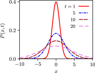
FIGURE 1. The distribution (7) at different times, showing the broadening of the distribution with time. Here, we have taken x₀ = 0.0, D = 0.5.

The mean-squared displacement (MSD) of the particle about its initial location is obtained straightforwardly from Eq. 7 as

$⟨{\left(x-x_0\right)}^2⟩\left(t\right)={\int }_{-\infty }^{\infty }\mathrm{d}x{\left(x-x_0\right)}^{2}P\left(x,t\right)=2Dt,(8)$

matching with the result (4), and which implies that the MSD grows forever as a function of time. Such a behavior in which the MSD grows linearly in time is referred to as normal diffusive behavior.

The aspect of the probability of finding the particle far off from x₀ increasing with time may be traced back to the fact that since the particle is diffusing in free space, it is no wonder that at longer times, it would have spread to a larger region of the available space than at shorter times. Let us then ask this question: Is there a way to stop this spread? Well, one possible way could be to have the particle diffuse not in free space but in a bounded domain of finite extent, say, between points x = − L and x = + L on the x-axis. In this case, the probability of finding the particle at a given location would keep increasing with time, until it can increase no further, that is, until the system attains a stationary state. In this state, attained in the limit t → ∞, it may be argued that this probability would be the same at all locations inside the bounded domain. In other words, the particle would be equally likely to be found anywhere within the region x ∈ [ − L, L].

Brownian Motion in Presence of Resetting

In the above backdrop, one may ask: Is there a way to induce a stationary state in the system by not tweaking the boundary conditions but by modifying the dynamics in a way that it continues to take place in the free space and yet has a stationary state? Of course, one way could be to subject the motion of the particle to take place in a bounded potential. In this respect, tweaking the boundary condition so that the particle diffuses not in free space but in a bounded domain of finite extent is tantamount to a potential that is zero everywhere except at the boundaries where one has an infinitely-high potential barrier. As an interesting alternative to using a potential, it turns out that there is a rather simple and instructive way to achieve the goal of inducing a stationary state, through the introduction of stochastic resetting in the dynamics [2]. To this end, let us modify the dynamics of free diffusion by stipulating that the particle in addition to evolving according to the rule (1) has also the option of resetting its position to its initial value. More specifically, at time t, the particle has in the ensuing infinitesimal time interval dt the following options for updating its location x(t): with probability rdt, it resets its position to initial value x₀, while with the complementary probability 1 − rdt, it evolves according to Eq. 1. Thus, we have [2]:

$x\left(t+\mathrm{d}t\right)=\left\{\begin{array}{cc}{x}_0\hfill & \mathrm{w}\mathrm{i}\mathrm{t}\mathrm{h}\mathrm{p}\mathrm{r}\mathrm{o}\mathrm{b}.r\mathrm{d}t,\hfill \\ x\left(t\right)+\eta \left(t\right)\mathrm{d}t\hfill & \mathrm{w}\mathrm{i}\mathrm{t}\mathrm{h}\mathrm{p}\mathrm{r}\mathrm{o}\mathrm{b}.1-r\mathrm{d}t.\hfill \end{array}\right.(9)$

Here, r ≥ 0 is a dynamical parameter, whose value when set to zero reduces the modified dynamics to that of free diffusion. In practical terms, a typical trajectory of the particle would involve free diffusion interspersed with events of reset to x₀, as shown in Figure 2. It is evident from Eq. 9 that introducing resetting into the dynamics (1) retains the Markov nature of the dynamics.

FIGURE 2

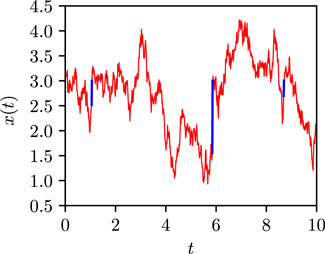
FIGURE 2. The plot shows a typical trajectory of a particle starting at location x₀ = 3.0 and performing free diffusion in one dimension, with stochastic resets to x₀ at random times. The parameter values are D = 0.5, and r = 0.25. The jumps in x values corresponding to resets are marked in blue.

Position Probability Distribution

Suppose we ask: what is the probability for the next reset to happen after a certain time t, in the interval [t, t + dt]? Let us discretize time in equal steps of length 0 < Δt ≪ 1; we will eventually consider the limit Δt → 0. The number of such steps during time duration t is obviously given by $\mathcal{N}=t/\mathrm{\Delta }t$. During each step of length Δt, the probability of reset equals rΔt, while the same for no reset equals 1 − rΔt. Consequently, the probability that the next reset happens after time t, in the interval [t, t + Δt], is given by $\stackrel{︸}{(1-r\mathrm{\Delta }t)}{}^{\mathcal{N}}r\mathrm{\Delta }t={(1-r\mathrm{\Delta }t)}^{t/\mathrm{\Delta }t}r\mathrm{\Delta }t$. In the limit Δt → 0, the latter quantity equals exp( − rt) rdt. We thus conclude that the probability for no reset to occur during a given time duration t equals exp( − rt), while the probability for the next reset to occur after time t, that is, in the interval [t, t + dt], equals exp( − rt) rdt. For latter purpose, let us note that at a given time instant t, the probability that the last reset happened in the interval [t − τ − dτ, t − τ], with τ ∈ [0, t], equals exp( − rτ) rdτ.

Note that as mentioned earlier, the dynamics (1) represents infinitesimal change in x in infinitesimal time interval dt, while incorporating resetting into the dynamics has in the resulting dynamics reset events leading to any amount of change in x in infinitesimal interval dt. Indeed, the reset destination is always the same, namely, x₀, irrespective of the location the particle resets from, so that the particle may execute a very long jump during a reset event.

It should be apparent from the aforementioned dynamical rules that introducing resetting into the dynamics would not let the particle go at any time, long or short, very far from the initial location. Is it actually the case? To answer this, we need to study just as in the case of free diffusion discussed above the time evolution of the probability density P_r(x, t) in presence of resetting, which may be derived by writing down the ways in which P_r(x, t) changes in a small time 0 < Δt ≪ 1 and then taking the limit Δt → 0. One has

$\begin{array}{ll}\hfill P_{\text{r}}\left(x,t+\mathrm{\Delta }t\right)& =P_{\text{r}}\left(x,t\right)+\left(1-r\mathrm{\Delta }t\right)[\int \mathrm{d}\left(\mathrm{\Delta }x\right)P_{\text{r}}\left(x-\mathrm{\Delta }x,t\right){\varphi }_{\mathrm{\Delta }t}\left(\mathrm{\Delta }x\right)-\int \mathrm{d}\left(\mathrm{\Delta }x\right)P_{\text{r}}\left(x,t\right){\varphi }_{\mathrm{\Delta }t}\left(\mathrm{\Delta }x\right)]\hfill \\ \hfill & -r\mathrm{\Delta }t{P}_{\text{r}}\left(x,t\right)+r\mathrm{\Delta }t\delta \left(x-x_0\right).\hfill \end{array}\left(10\right)$

Here, the second and the third term arise from diffusion, while the fourth and the fifth term are owing to resetting events. While the former two terms are as in the free diffusion case, Eq. 6, the latter two terms may be understood as follows. For r ≠ 0, there is a loss in probability at all locations other than x₀ due to resetting events, which is represented by the fourth term on the rhs of Eq. 10, while the corresponding gain in probability at x = x₀, given by rΔtδ(x − x₀)∫dx P_r(x, t) = rΔtδ(x − x₀), yields the last term on the rhs. Here we have used the normalization condition ∫dx P_r(x, t) = 1 ∀ t. Implementing appropriate Taylor expansions on both sides of Eq. 10, then taking the limit Δt → 0, the probability P_r(x, t) may be shown to be satisfying the Fokker-Planck equation [2]

$\frac{\partial P_{\text{r}}\left(x,t\right)}{\partial t}=D\frac{{\partial }^2{P}_{\text{r}}\left(x,t\right)}{\partial x^2}-r{P}_{\text{r}}\left(x,t\right)+r\delta \left(x-x_0\right).(11)$

The initial condition is P_r(x, 0) = δ(x − x₀). Eq. 11 may be solved for P_r(x, t); here, we report only the solution, referring the reader to Ref. [3] for details of obtaining it:

$\begin{array}{ll}\hfill P_{\text{r}}\left(x,t\right)& =\frac{e^{-rt-\frac{{\left(x-x_0\right)}^2}{4Dt}}}{\sqrt{4\pi Dt}}+\frac{1}{4}\sqrt{\frac{r}{D}}{e}^{-\sqrt{\frac{r}{D}}|x-x_0|}\mathrm{E}\mathrm{r}\mathrm{f}\mathrm{c}\left(\frac{|x-x_0|}{2\sqrt{Dt}}-\sqrt{rt}\right)\hfill \\ \hfill & -\frac{1}{4}\sqrt{\frac{r}{D}}{e}^{\sqrt{\frac{r}{D}}|x-x_0|}\mathrm{E}\mathrm{r}\mathrm{f}\mathrm{c}\left(\frac{|x-x_0|}{2\sqrt{Dt}}+\sqrt{rt}\right),\hfill \end{array}(12)$

where $\mathrm{E}\mathrm{r}\mathrm{f}\mathrm{c}(x)\equiv 2/\left(\sqrt{\pi }\right){\int }_x^{\infty }\mathrm{d}y{e}^{-y^2}$ is the complementary error function. The MSD of the particle may be obtained from Eq. 12 as

$⟨{\left(x-x_0\right)}^2⟩\left(t\right)=\frac{2D}{r}\left(1-e^{-rt}\right).(13)$

Eq. 12 implies that in the limit t → ∞, one has a stationary-state form [2]:

$P_{\text{r,\hspace{0.17em}ss}}\left(x\right)=\frac{1}{2}\sqrt{\frac{r}{D}}{e}^{-|x-x_0|\sqrt{r/D}}.(14)$

Correspondingly, the MSD relaxes at long times to the stationary-state value

${⟨{\left(x-x_0\right)}^2⟩}_{\text{r,\hspace{0.17em}ss}}=\frac{2D}{r}.(15)$

Figure 3 shows the probability distribution P_r(x, t) in presence of resetting and at four different times, as given by Eq. 12, showing in particular convergence in time to the stationary state (14).

The stationary-state distribution is an exponential centred at the resetting location; since the particle keeps resetting to x₀ in time, it is no wonder that the most likely position of the particle is x₀. More importantly, an exponential profile implies that there is a characteristic length scale within which the particle is to be found with significant probability and beyond which one has an exponentially-small probability of finding the particle. In conclusion, we have been able to achieve our goal: by modifying not the boundary conditions but rather the dynamics of free diffusion, one induces a stationary state in the system. While we have discussed in the foregoing the case of resetting at exponentially-distributed random times, the case of resetting at power-law-distributed random times has also been considered in the literature, see Ref. [4]. We remark in passing that resetting creates a source of probability at x₀ and a sink at all other locations x ≠ x₀, so that the condition of detailed balance, which characterizes an equilibrium stationary state [5], is manifestly violated in the stationary state induced by resetting. Consequently, the stationary state (14) is a generic nonequilibrium stationary state [2].

FIGURE 3

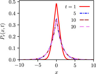
FIGURE 3. Probability distribution P_r(x,t) in presence of resetting and at four different times, as given by Eq. 12, showing convergence in time to a stationary state in which the distribution no longer changes with time. The latter is given by Eq. 14. The parameter values are x₀ = 0.0, D = 0.5, and r = 0.25.

First-Passage Time Distribution

Now that we have seen a stationary state emerging in presence of stochastic resetting, one may wonder if besides this issue of theoretical relevance there is any practical utility of the process of stochastic resetting. Here, we will discuss one very interesting application of stochastic resetting, namely, in the context of search processes.

The Case of Brownian Motion

In order to discuss the concept and utility of first-passage times, let us come back to free diffusion. Referring to Figure 4, suppose we ask: when does a trajectory of free diffusion starting at x₀ > 0 at time t = 0 cross the origin for the first time? Clearly the time t_f that it happens, aptly termed the first-passage time (FPT), is a random variable that varies from trajectory to trajectory, and one may ask: what is the form of its distribution $\mathcal{P}(x_0,t_f)$ ? This distribution would explicitly depend on x₀, a fact encoded in the defining symbol for the distribution. In order to answer this question, noting that t_f is by definition a positive quantity, it proves convenient to consider the Laplace transform of $\mathcal{P}(x_0,t_f)$:

$\tilde{\mathcal{P}}\left(x_0,s\right)\equiv {\int }_0^{\infty }\mathrm{d}{t}_f{e}^{-s{t}_f}\mathcal{P}\left(x_0,t_f\right)=⟨e^{-s{t}_f}⟩,(16)$

where the angular brackets denote averaging with respect to the distribution $\mathcal{P}(x_0,t_f)$, s is the Laplace variable, and tilde denotes the function obtained on performing Laplace transform $\mathcal{L}$ of a function f(t), that is, $\mathcal{L}[f(t)]=\tilde{f}(s)$. Now, let us understand that a given value of t_f corresponds to all trajectories ${\{x(\tau )\}}_{0\le \tau \le t_f}$ between times 0 and t_f satisfying x(0) = x₀ and x(0 < τ < t_f) > 0. Consequently, averaging with respect to t_f is tantamount to averaging with respect to all trajectories that start at x₀ and propagate for time t_f without ever crossing the origin, and such an averaging is what the angular brackets in Eq. 16 would also stand for.

In order to proceed, we now derive a differential equation for $\tilde{\mathcal{P}}(x_0,s)$. To this end, following Ref. [6], we split the time interval [0, t_f] into two parts. During the first interval [0, Δτ], the aforementioned set of trajectories start from x₀ and propagate up to x₀ + Δx, where Δx is of course different for different trajectories. In the second interval [Δτ, t_f], these trajectories start at x₀ + Δx and reach 0 at t_f. We take Δτ to be a small time interval with 0 < Δτ ≪ 1, and eventually, we would take the limit Δτ → 0. We get, to leading order in Δτ, that

$\tilde{\mathcal{P}}\left(x_0,s\right)=e^{-s\mathrm{\Delta }\tau }{⟨\tilde{\mathcal{P}}\left(x_0+\mathrm{\Delta }x,s\right)⟩}_{\mathrm{\Delta }x}\approx \left(1-s\mathrm{\Delta }\tau \right){⟨\tilde{\mathcal{P}}\left(x_0+\mathrm{\Delta }x,s\right)⟩}_{\mathrm{\Delta }x},(17)$

where the average denoted by the angular brackets is to be performed over all realizations of Δx. Now, Δτ being small implies that so is Δx, so that the quantity $\tilde{\mathcal{P}}(x_0+\mathrm{\Delta }x,s)$ on the rhs of the above equation may be expanded in a Taylor series in Δx. One gets

$\tilde{\mathcal{P}}\left(x_0,s\right)\approx \left(1-s\mathrm{\Delta }\tau \right){⟨\tilde{\mathcal{P}}\left(x_0,s\right)+{\tilde{\mathcal{P}}}^{\prime }\left(x_0,s\right)\mathrm{\Delta }x+{\tilde{\mathcal{P}}}^{″}\left(x_0,s\right)\frac{{\left(\mathrm{\Delta }x\right)}^2}{2}+\cdots ⟩}_{\mathrm{\Delta }x}.(18)$

Here, the prime denotes derivative with respect to x₀. Now, Eq. 1 gives Δx = η(0)Δτ, so that averaging with respect to Δx is equivalent to averaging with respect to different realizations of η(0). Using ⟨η(0)⟩ = 0 and ⟨η²(0)⟩ = 2D/Δτ (see Appendix) so that ⟨Δx⟩_Δx = 0 and ${⟨{(\mathrm{\Delta }x)}^2⟩}_{\mathrm{\Delta }x}=2D\mathrm{\Delta }\tau$, we get from Eq. 18 on taking the limit Δτ → 0 that

$D{\tilde{\mathcal{P}}}^{″}\left(x_0,s\right)-s\tilde{\mathcal{P}}\left(x_0,s\right)=0.(19)$

The above equation, referred to as the backward Fokker-Planck equation, is to be solved subject to two boundary conditions: 1) $\tilde{\mathcal{P}}(x_0\to 0,s)=1$, since as x₀ → 0, we have t_f → 0, and 2) $\tilde{\mathcal{P}}(x_0\to \infty ,s)=0$, since as x₀ → ∞, we have t_f → ∞. The solution of Eq. 19 subject to these boundary conditions is

$\tilde{\mathcal{P}}\left(x_0,s\right)=e^{-\sqrt{s/D}{x}_0}.(20)$

On performing inverse Laplace transformation, one readily gets [6].

$\mathcal{P}\left(x_0,t_f\right)=\frac{x_0}{\sqrt{4\pi D}}\frac{e^{-x_0^2/\left(4D{t}_f\right)}}{t_f^{3/2}}.(21)$

(For x₀ < 0, the corresponding FPT distribution is obtained from the above equation with the replacement x₀ → |x₀|.) We thus find that the FPT distribution has a tail $\sim t_f^{-3/2}$, and moreover, that the average FPT (the mean first-passage time (MFPT)) given by $⟨t_f⟩={\int }_0^{\infty }\mathrm{d}{t}_f{t}_f\mathcal{P}(x_0,t_f)$ is infinite ! The latter result implies that the dynamics (1) allows for trajectories which starting at x₀ start to move away from the origin and hence take a very long time to hit the origin for the first time (e.g., the blue trajectory in Figure 4). Does repeated resetting to x₀ kill these trajectories, given that it allows the particle to remain effectively in a finite region around x₀? Let us then investigate the distribution of the FPT in presence of resetting.

FIGURE 4

FIGURE 4. Two sample trajectories x(t) corresponding to free diffusion (1) with initial condition x(0) = x₀ = 3.0, and with D = 0.5. Here, the quantity t_f is the first-passage time for the red trajectory.

The Case of Brownian Motion in Presence of Resetting

In order to proceed, define ${\mathcal{P}}_{\text{r}}(x_0,t_f)$ as the FPT distribution in presence of resetting, and S_r(x₀, t) as the so-called survival probability, that is, the probability that a trajectory starting at x₀ at time t = 0 has not crossed the origin up to time t. Note that resetting is taking place not to the origin but to the initial location x₀ of the particle. Obviously then one has $S_{\text{r}}(x_0,t+\mathrm{\Delta }t)-S_{\text{r}}(x_0,t)={\mathcal{P}}_{\text{r}}(x_0,t)\mathrm{\Delta }t$ for small Δt, which in the limit Δt → 0 gives ${\mathcal{P}}_{\text{r}}(x_0,t)=-\partial S_{\text{r}}(x_0,t)/\partial t$. In terms of S_r(x₀, t), the mean FPT is given as ${⟨t_f⟩}_{\text{r}}\equiv {\int }_0^{\infty }\mathrm{d}{t}_f{t}_f{\mathcal{P}}_{\text{r}}(x_0,t_f)=-{\int }_0^{\infty }\mathrm{d}{t}_f{t}_f\partial S_{\text{r}}(x_0,t_f)/\partial t_f=-{[t_f{S}_{\text{r}}(x_0,t_f)]}_0^{\infty }+{\int }_0^{\infty }\mathrm{d}{t}_f{S}_{\text{r}}(x_0,t_f)={\int }_0^{\infty }\mathrm{d}{t}_f{S}_{\text{r}}(x_0,t_f)={\tilde{S}}_{\text{r}}(x_0,s=0)$, using S_r(x₀, ∞) = 0. A trajectory starting from x₀ that reaches the origin for the first time at time t may have had no reset at all since the time instant t = 0 or may have had its last reset at an earlier time instant in the interval [t − τ − dτ, t − τ], with τ ∈ [0, t], and has not passed through the origin before that. Consequently, one has

${\mathcal{P}}_{\text{r}}\left(x_0,t\right)=-\frac{\partial S_{\text{r}}\left(x_0,t\right)}{\partial x_0}={\int }_0^t\mathrm{d}\tau S_{\text{r}}\left(x_0,t-\tau \right)r{e}^{-r\tau }\mathcal{P}\left(x_0,\tau \right)+e^{-rt}\mathcal{P}\left(x_0,t\right).(22)$

Indeed, trajectories that did not have any reset during the time interval [0, t] (the probability of which, according to our earlier discussions, is exp( − rt)) give rise to the second term on the rhs of the second equality above. On the other hand, trajectories that at time t have had last reset in the interval [t − τ − dτ, t − τ] (the probability of which is exp( − rτ) rdτ), with τ ∈ [0, t], and have not hit the origin before that give rise to the first term on the rhs of the second equality.

Using Eq. 21 in Eq. 22, taking Laplace transform of both sides, and using S_r(x₀, t = 0) = 1, we finally get

$\tilde{S}\left(x_0,s\right)=\frac{1-A}{rA+s},(23)$

where the quantity A is defined as

$A\equiv A\left(s,r\right)=\mathcal{L}\left[\frac{x_0{e}^{-rt-x_0^2/\left(4Dt\right)}}{\sqrt{4\pi D{t}^3}}\right]=e^{-\sqrt{\left(x_0^2/D\right)\left(s+r\right)}}.(24)$

Here, we have used $\mathcal{L}[t^{-3/2}\exp (-a/(4t))]=2\sqrt{\pi /a}\exp (-\sqrt{as})$ for Re(a) > 0. Consequently, we obtain the MFPT in presence of resetting as [2].

${⟨t_f⟩}_{\text{r}}=\frac{e^{x_0\sqrt{r/D}}-1}{r}.(25)$

We see from Eq. 25 that for fixed x₀ and D, the MFPT in presence of resetting is finite for finite r, so that resetting has a drastic consequence on rendering the MFPT of free diffusion finite. Moreover, ${⟨t_f⟩}_{\text{r}}$ diverges in two extreme limits, namely, as r → 0 and as r → ∞, so it has to be that there exists a value r^⋆ of r at which ${⟨t_f⟩}_{\text{r}}$ as a function of r has a minimum. Note that the limit r → 0 corresponds to free diffusion, so that the fact of a diverging ${⟨t_f⟩}_{\text{r}}$ as r → 0 is consistent with what we observed above regarding the MFPT for free diffusion. The divergence of MFPT as r → ∞ may be understood on the basis of the fact that in this limit, the particle resets so often that it does not effectively get a chance to move away from x₀ and hit the origin. The quantity r^⋆ satisfying $\mathrm{d}{⟨t_f⟩}_{\text{r}}/\mathrm{d}r{|}_{r=r^{\star }}=0$ yields the following transcendental equation [2].

$\frac{z^{\star }}{2}=1-e^{-z^{\star }};r^{\star }={\left(z^{\star }\right)}^{2}D/x_0^2,(26)$

which has a unique non-zero solution z^⋆ = 1.593 62 …. It then follows that there is an optimal resetting rate r^⋆, such that the MFPT in presence of resetting attains its minimum as a function of r. The variation of ${⟨t_f⟩}_{\text{r}}$ with r, as given by Eq. 25, is shown in Figure 5, which clearly shows the existence of a minimum.

FIGURE 5

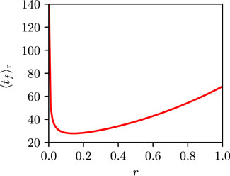
FIGURE 5. The mean first-passage time in presence of resetting given by Eq. (25) is shown as a function of r for x₀ = 3.0 and D = 0.5. One may observe the existence of a distinct minimum.

Relevance of Resetting in Search Processes

What has then a minimum MFPT got to do with search processes? Imagine having misplaced one of your favourite or essential belongings. It could be your car key or your mobile phone. After getting into your office, you usually keep the key on your office table. Having misplaced it, a typical tendency to locate it is to begin searching in random directions for the key (well, you do not know beforehand which particular direction to search for, so random directions would be the best bet!) while starting from your office. Having searched unsuccessfully for sometime, you realize that perhaps you did not search well enough in the region around the table (after all, you usually keep the key on the table itself), so you return to the table, and re-initiate your search. You keep repeating the process until you locate the key, and of course the first time you locate it, you stop searching any further. Figure 6 models this search strategy in one dimension: the brown filled circle denotes your misplaced belonging, while searching in random directions for random times followed by re-initiation of the search process from your starting position may be modelled as free diffusion interspersed in time with stochastic resets to the initial location (the two space-time trajectories in the plot), namely, what has been our model of study in this work. Had there been no resets, that is, if you had continued searching in random directions without ever coming back to your initial location, we would arrive at the following conclusion based on our analysis of free diffusion pursued above. If you had repeated the process over and over again, then, in some realizations of the process, you would have located the brown circle in a finite time, while there would be happily a large number of other realizations in which you fail to locate it in finite time, so that the MFPT through the brown circle would diverge ! On the other hand, introducing stochastic resetting into the dynamics would make the MFPT finite, as our theoretical analysis of diffusion with stochastic resetting has revealed. Not just that, there exists an optimal value for the rate r at which stochastic resets are executed such that the corresponding MFPT attains its minimum value. Thus, stochastic resetting offers a very efficient way to locate your misplaced belonging. Of course, for resetting to be efficient, the quantity x₀, the initial location of the searcher to which it repeatedly resets, has to be small enough. In other words, the location x₀ has to be close enough to the target for resetting to do a good job. Indeed, as is evident from Eq. 25, if x₀ is large, the MFPT would be very large, and then resetting would not help to locate the target in a finite time.

FIGURE 6

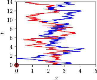
FIGURE 6. The plot shows a stationary target (misplaced belonging) denoted by the brown filled circle and located at the origin, and two space-time trajectories of a particle starting from x₀ = 2.5 and executing stochastic resets to x₀ at random times. The parameter values are D = 0.5 and r = 0.25. From the figure, we see that one of the trajectories has been able to detect the target, while the other one is yet to locate it.

Stochastic Thermodynamics of Resetting

In this section, we review briefly thermodynamics of systems subject to stochastic resetting, following Refs. [7, 8], and using basic principles extending thermodynamic laws to nonequilibrium systems laid down and reviewed in Ref. [9]. Consider first a Markov process in which the state space instead of being continuous, as in Eq. 1, is discrete. Let us denote the latter by non-zero integers i. The set of all possible states spans the state space of the system. Let N be the total number of states accessible to the system. The dynamics of the system is dictated by a set of transition rates W_i→j ≥ 0 giving the probability per unit time for the system to make a transition from state i to state j. We consider these transition rates to be time-independent. Define p_i(t) to be the probability for the system to be in state i at time t, with the normalization ${\sum }_{i=1}^N{p}_i(t)=1\forall t$. These probabilities evolve in time following the so-called Master equation [5]

$\frac{\mathrm{d}{p}_i\left(t\right)}{\mathrm{d}t}=\sum _{j=1}^N\left[W_{j\to i}{p}_j\left(t\right)-W_{i\to j}{p}_i\left(t\right)\right],(27)$

where the first term (respectively, the second term) on the right hand side summarizes all possible ways in which p_i(t) increases (respectively, decreases) in an infinitesimal time interval [t, t + dt] due to transitions from all states j to the state i in question (respectively, due to transitions from state i to states j). Note that the Master Eq. 27 conserves in time the normalization of the probability p_i(t). Let us note that the Brownian motion (1) may be considered as the continuous-space limit of a discrete-space continuous-time random walker moving with equal probability between the nearest-neighbour sites of a one-dimensional lattice [5]; in the latter case, the state space is constituted by the site indices, and we have W_i→j = W_j→i.

Now, for a given pair of states i and j, consider the following situation [8]: 1) Both the forward and backward transitions are allowed (denote the corresponding transition rates by W_i→j ≡ w_i→j > 0 and W_j→i ≡ w_j→i > 0). 2) Either the forward or the backward transition is allowed but not both (i.e., either we have W_i→j ≡ y_i→j > 0 and W_j→i ≡ y_j→i = 0, or, W_j→i ≡ y_j→i > 0 and W_i→j ≡ y_i→j = 0). The former dynamics is known as the bidirectional process, while the latter is referred to as the unidirectional process [8]. The reason we want to focus on this specific situation is that it models the resetting dynamics considered in this work. Indeed, a given state x(t) can in an infinitesimal time interval [t, t + dt] evolve to any other x value allowed by the dynamics (1), just as any other x value can evolve to the given value x(t) in an infinitesimal time interval [t, t + dt] provided of course the dynamics (1) allows that. On the contrary, the resetting dynamics is such that in an infinitesimal time interval [t, t + dt], any x value can evolve to the value x₀, but the reverse move from x₀ to any other x value via the resetting dynamics is not allowed (it is allowed only via the Brownian motion dynamics (1)). The Master Eq. 27 then reads [8].

$\frac{\mathrm{d}{p}_i\left(t\right)}{\mathrm{d}t}=\sum _{j=1}^N\left[w_{j\to i}{p}_j\left(t\right)-w_{i\to j}{p}_i\left(t\right)\right]+\sum _{j=1}^N\left[y_{j\to i}{p}_j\left(t\right)-y_{i\to j}{p}_i\left(t\right)\right],(28)$

where the summation in the second term on the right hand side is considered restricted to those pair of states for which the reverse transitions are not allowed (i.e., either we have y_i→j > 0 and y_j→i = 0, or, y_j→i > 0 and y_i→j = 0).

The (Shannon) entropy of the system at time t is given by (we work in units in which the Boltzmann constant is set to unity):

$S_{\text{sys}}\left(t\right)=-\sum _{i=1}^N{p}_i\left(t\right)\ln p_i\left(t\right),(29)$

where p_i(t) is to be obtained by solving the Master Eq. 28 subject to a given initial condition ${\{p_i(0)\}}_{1\le i\le N}$. Differentiating the above equation with respect to time, using Eq. 28, and the normalization ${\sum }_{i=1}^N{p}_i(t)=1$ yield straightforwardly the entropy production rate for the system [8]:

${\dot{S}}_{\text{sys}}\left(t\right)=\sum _{i,j=1}^N{w}_{j\to i}{p}_j\left(t\right)\ln \left(\frac{p_j\left(t\right)}{p_i\left(t\right)}\right)+\sum _{i,j=1}^N{y}_{j\to i}{p}_j\left(t\right)\ln \left(\frac{p_j\left(t\right)}{p_i\left(t\right)}\right),(30)$

where the dot denotes derivative with respect to time.

Let us for the moment disregard any resetting-like transitions in the system. Eq. 30 then reads

${\dot{S}}_{\text{sys}}\left(t\right)=\sum _{i,j=1}^N{w}_{j\to i}{p}_j\left(t\right)\ln \left(\frac{p_j\left(t\right)}{p_i\left(t\right)}\right)=\sum _{i,j=1}^N{w}_{j\to i}{p}_j\left(t\right)\ln \left(\frac{w_{j\to i}{p}_j\left(t\right)}{w_{i\to j}{p}_i\left(t\right)}\right)-{\dot{S}}_{\text{env}}\left(t\right);(31)$

${\dot{S}}_{\text{env}}\left(t\right)\equiv \sum _{i,j=1}^N{w}_{j\to i}{p}_j\left(t\right)\ln \left(\frac{w_{j\to i}}{w_{i\to j}}\right).(32)$

In the above, we have defined ${\dot{S}}_{\text{env}}$ as the environment entropy production, related to the change in entropy of the environment corresponding to the system making transitions from every state j to every state i. Here, the understanding is that it is the interaction with the environment that induces transitions between the states of the system, just as in the dynamics (1), the variable x evolves in time due to the noise η(t) arising because of the presence of the environment constituted by the surrounding fluid. Eq. 31 then yields the total entropy production rate as

$\begin{array}{ll}\hfill {\dot{S}}^{\text{tot}}\left(t\right)& \equiv {\dot{S}}_{\text{sys}}\left(t\right)+{\dot{S}}_{\text{env}}\left(t\right)\hfill \\ \hfill & =\sum _{i,j=1}^N{w}_{j\to i}{p}_j\left(t\right)\ln \left(\frac{w_{j\to i}{p}_j\left(t\right)}{w_{i\to j}{p}_i\left(t\right)}\right)\hfill \\ \hfill & =\frac{1}{2}\sum _{i,j=1}^N\left(w_{j\to i}{p}_j\left(t\right)-w_{i\to j}{p}_i\left(t\right)\right)\ln \left(\frac{w_{j\to i}{p}_j\left(t\right)}{w_{i\to j}{p}_i\left(t\right)}\right)\ge 0.\hfill \end{array}(33)$

That ${\dot{S}}^{\text{tot}}(t)\ge 0$ may be understood by noting that (x − y) ln(x/y) ≥ 0 for any real, positive x, y and that f ln f = 0 for f = 0. The above expression for ${\dot{S}}^{\text{tot}}$ is the Schnakenberg’s formula for the total entropy production of the system [8].

In presence of resetting, Eq. 30 then leads to

${\dot{S}}^{\text{tot}}\left(t\right)={\dot{S}}_{\text{sys}}\left(t\right)+{\dot{S}}_{\text{env}}\left(t\right)-{\dot{S}}_{\text{reset}}\left(t\right);(34)$

${\dot{S}}_{\text{reset}}\left(t\right)\equiv \sum _{i,j=1}^N{y}_{j\to i}{p}_j\left(t\right)\ln \left(\frac{p_j\left(t\right)}{p_i\left(t\right)}\right),(35)$

where we have defined ${\dot{S}}_{\text{reset}}(t)$ as the entropy production rate due to unidirectional processes, i.e., resetting-like transitions. For the case when the system resets to a state i₀ from any state j with a resetting rate r_j, we have

${\dot{S}}_{\text{reset}}\left(t\right)=\sum _{j=1}^N{r}_j{p}_j\left(t\right)\ln \left(\frac{p_j\left(t\right)}{p_{i_0}\left(t\right)}\right)={\dot{S}}_{\text{reset}}^{\text{abs}}\left(t\right)+{\dot{S}}_{\text{reset}}^{\text{ins}}\left(t\right);(36)$

${\dot{S}}_{\text{reset}}^{\text{abs}}\left(t\right)\equiv \sum _{j=1}^N{r}_j{p}_j\left(t\right)\ln \left(p_j\left(t\right)\right),(37)$

${\dot{S}}_{\text{reset}}^{\text{ins}}\left(t\right)\equiv -\ln \left(p_{i_0}\left(t\right)\right)\sum _{j=1}^N{r}_j{p}_j\left(t\right).(38)$

Here, ${\dot{S}}_{\text{reset}}^{\text{abs}}(t)$ is the absorption entropy rate, corresponding to the change in the Shannon entropy of the system due to the probability flux out of every state j owing to resetting. On the other hand, the quantity ${\dot{S}}_{\text{reset}}^{\text{ins}}(t)$ is the insertion entropy rate that depends on the probability at the resetting state i₀ and the probability flux out of every other state j [7].

In a stationary state, all the quantities ${\dot{S}}_{\text{sys}}$, ${\dot{S}}_{\text{env}}$, ${\dot{S}}^{\text{tot}}$, ${\dot{S}}_{\text{reset}}$, etc are time independent, and moreover, ${\dot{S}}_{\text{sys}}=0$ by construction. Hence, with ${\dot{S}}^{\text{tot}}\ge 0$, we get from Eq. 34 that

${\dot{S}}^{\text{tot}}={\dot{S}}_{\text{env}}-{\dot{S}}_{\text{reset}}\ge 0.(39)$

In an equilibrium stationary state, which is obtained in the absence of resetting (see the paragraphs following Eq. 15), one has the condition of detailed balance, w_j→i p_j = w_i→j p_i for all pairs of states i and j with time-independent p_i’s. Consequently, one has ${\dot{S}}^{\text{tot}}=0$, and Eq. 39 implies that ${\dot{S}}_{\text{env}}=0$. One may have time-independent p_i’s (i.e., a stationary state) with violation of detailed balance; this leads to a non-vanishing ${\dot{S}}^{\text{tot}}$, which is thus a fingerprint of non-equilibrium stationary states. Resetting induces such a state, and hence, in a nonequilibrium stationary state induced by resetting, one would have

${\dot{S}}_{\text{env}}-{\dot{S}}_{\text{reset}}>0,(40)$

which is interpreted as the second law of thermodynamics in presence of resetting [7]. Considering the particular example of a discrete-space continuous-time random walker, for which one has w_i→j = w_j→i, we have ${\dot{S}}_{\text{env}}=0$, and hence that ${\dot{S}}_{\text{reset}}<0$. This result should also apply to the dynamics (1) in presence of resetting, as we will demonstrate in the following.

Eq. 36 when generalized to a Markov process with continuous state space reads [7].

${\dot{S}}_{\text{reset}}\left(t\right)=\int \mathrm{d}xr\left(x\right)P_{\text{r}}\left(x,t\right)\ln \left(\frac{P_{\text{r}}\left(x,t\right)}{P_{\text{r}}\left(x_0,t\right)}\right).(41)$

For the case r(x) = r, a space-independent resetting rate, the situation we have considered in this work (see Eq. 9), we get

${\dot{S}}_{\text{reset}}\left(t\right)=r\int \mathrm{d}x{P}_{\text{r}}\left(x,t\right)\ln \left(\frac{P_{\text{r}}\left(x,t\right)}{P_{\text{r}}\left(x_0,t\right)}\right).(42)$

In the nonequilibrium stationary state (14), we get

${\dot{S}}_{\text{reset}}=-\frac{r}{2}{\int }_{-\infty }^{\infty }\mathrm{d}y|y-y_0|e^{-|y-y_0|}=-r.(43)$

We thus see explicitly that we have ${\dot{S}}_{\text{reset}}<0$ in the nonequilibrium stationary state induced in the Brownian dynamics due to resetting. That the resetting entropy decreases in time is a reflection of the fact that what resetting essentially does is to reduce the uncertainty in the particle position. To wrap up this part, we mention a few relevant recent work dealing with thermodynamics of resetting: Ref. [10] that discusses the validity of the so-called integral fluctuation theorems in presence of stochastic resetting, Ref. [11] that considers an overdamped Brownian particle in a potential well modulated through an external protocol and subject to stochastic resetting and studies the fluctuations of the work done on the system, Ref. [12] that derives a thermodynamic relation for systems with unidirectional transitions including in particular a random walk subject to stochastic resetting.

In closing this section, we indicate how resetting may play a role in optimizing the efficiency of stochastic heat engines. We first describe briefly the principle of working of a stochastic heat engine constituted by a Brownian particle of mass m, which is placed in a fluid medium in equilibrium at a given temperature, thereby modelling a heat bath or a thermal reservoir [13]. For simplicity, let us consider the motion of the particle in one dimension x. The particle is subject to trapping due to an attractive force derived from a time-dependent potential U(x(t); t) and is also acted upon by a time-dependent non-conservative force F(x(t); t). The position x(t) and the velocity v(t) = dx(t)/dt of the particle evolve in time following the underdamped Langevin dynamics:

$m\frac{{\mathrm{d}}^{2}x\left(t\right)}{\mathrm{d}{t}^2}=-\frac{\partial U\left(x\left(t\right);t\right)}{\partial x}+F\left(x\left(t\right);t\right)-\gamma \frac{\mathrm{d}x\left(t\right)}{\mathrm{d}t}+\xi \left(t\right),(44)$

where γ is the friction coefficient accounting for the friction that the particle experiences while moving in the surrounding medium, while ξ(t) models the random force that the surrounding fluid molecules impart on the particle. One models ξ(t) as a Gaussian, white noise with zero mean and correlations in time given by ⟨ξ(t)ξ(t′)⟩ = 2γTδ(t − t′), where T is the temperature of the fluid medium in units of the Boltzmann constant. Note that in the absence of the potential U(x(t); t) and the non-conservative force F(x(t); t), when one considers the limit of large damping (the limit γ/m → ∞ at a fixed and finite m), the dynamics (44) takes the form of the overdamped Langevin dynamics (1). The dynamics (44) is what is known to physicists as the Brownian motion, while mathematicians prefer to refer to the overdamped dynamics (1) as the Brownian motion.

In using system (44) as a heat engine, one allows the temperature of the surrounding fluid medium to switch between a higher temperature T_h and a lower temperature T_c, thus mimicking the hot and the cold thermal reservoir of an engine, respectively. A prominent example of an engine is the well-studied Carnot engine. Specifically, in our setup, considering U to be a harmonic potential, one varies the stiffness of this potential in time from times 0 to t₁ to implement the isothermal expansion at temperature T_h and from times t₁ to t₁ + t₃ to implement the isothermal compression at temperature T_c of a Carnot cycle, while the adiabatic expansion and compression stages of the latter may be implemented by performing an instantaneous change in the stiffness at time instants t₁ and t₁ + t₃, with concomitant jump in temperature from T_h to T_c and from T_c to T_h, respectively. Heat transfer takes place between the bath and the particle during the isothermal stages and not during the adiabatic stages. The aforementioned scenario defines a stochastic Carnot heat engine at the micro scale, with reasons of stochasticity being enhanced thermal fluctuations prevalent in the dynamics at such scales [14].

The heat transfer between the heat bath and the particle in time t and computed along the trajectory of the particle from x(0) to x(t) is given by

$Q\left(t\right)={\int }_{x\left(0\right)}^{x\left(t\right)}\left(-\gamma \frac{\mathrm{d}x\left(t^{\prime }\right)}{\mathrm{d}{t}^{\prime }}+\xi \left(t^{\prime }\right)\right)◦\mathrm{d}x\left(t^{\prime }\right),(45)$

where ° implies that the integral on the right hand side is to be evaluated in the Stratonovich sense [15]. Similarly, the work done on the particle in time t equals

$W\left(t\right)={\int }_0^t\frac{\partial U\left(x\left(t^{\prime }\right);t^{\prime }\right)}{\partial t^{\prime }}◦\mathrm{d}x\left(t^{\prime }\right)+{\int }_0^{t}F\left(x\left(t^{\prime }\right);t^{\prime }\right)◦\mathrm{d}x\left(t^{\prime }\right).(46)$

Note that both the heat and the work are stochastic functions of time that fluctuate between trajectories of the particle. Next, one invokes stochastic definition of efficiency as given by the ratio of the stochastic work extracted in a cycle to the stochastic heat transferred Q_h(t) from the hot bath to the particle in a cycle, as

$\eta \left(t\right)=-\frac{W\left(t\right)}{Q_h\left(t\right)},(47)$

where t denotes the total duration of the cycle. On considering the ratio of average quantities, the corresponding efficiency $\bar{\eta }(t)=-⟨W(t)⟩/⟨Q_h(t)⟩$ is bounded on the upper side by the second law of thermodynamics by η_C = 1 − T_c/T_h, with η_C being the Carnot efficiency. The challenge then is to engineer an optimal protocol for changing the stiffness of the potential U so as to maximize the efficiency $\bar{\eta }(t)$. Since the heat Q_h and the work W are functionals of the trajectories of the particle as generated by the dynamics (44), one may ask: is there a location x(0) or x(t) for which values of such quantities are optimised? In case it is so, does it then prove beneficial to implement repeated resetting of the position of the particle to such locations so as to achieve an enhanced efficiency of the engine? Considering resetting at exponential times (the set-up of Eq. 9), an issue of importance would be: is there an optimal resetting rate r for which one obtains maximum efficiency? Can one work out the stochastic energetics of the engine in presence of resetting? In the wake of recent surge in activity in the field of both stochastic thermodynamics and stochastic resetting, it is tempting to speculate that study of such questions, either in the framework outlined above or suitable modifications thereof, may yield useful and insightful results on the issue of optimization of thermal machines at micro scales. The perspectives presented here may serve as a genesis for future research in this direction.

Resetting of Scaled and Fractional Brownian Motion

Scaled Brownian Motion

Until now, we have considered standard Brownian motion (1) in discussing the effects of stochastic resetting. We now discuss briefly the corresponding effects on the so-called scaled Brownian motion (SBM) [16, 17], which in appropriate limits reduces to the standard Brownian motion. SBM is used in such contexts as fluorescence recovery following photobleaching [18], anomalous diffusion in biophysics [19, 20], granular gas of viscoelastic particles [21], etc. In contrast to the standard Brownian motion (1) that involves a time-independent diffusion coefficient, the SBM involves a diffusion coefficient that is time dependent and in fact which scales as a power-law in time. Thus, the corresponding dynamics is given by [16].

$\frac{\mathrm{d}x}{\mathrm{d}t}=\eta \left(t\right),(48)$

with η(t) a Gaussian, white noise with properties

$\langle \eta \left(t\right)\rangle =0,\langle \eta \left(t\right)\eta \left(t^{\prime }\right)\rangle =2D\left(t\right)\delta \left(t-t^{\prime }\right);(49)$

here, we have

$D\left(t\right)=\alpha K_{\alpha }{t}^{\alpha -1};\alpha >0,(50)$

with K_α a constant. Note that setting α = 1 and K₁ = D reduces the SBM to the standard BM (1). In the case of the SBM, the position probability distribution may be shown to have the form [16].

$P\left(x,t\right)=\frac{1}{\sqrt{4\pi K_{\alpha }{t}^{\alpha }}}{e}^{-{\left(x-x_0\right)}^2/\left(4K_{\alpha }{t}^{\alpha }\right)},(51)$

which as expected reduces for α = 1 to the result (7). The MSD for the SBM reads [16].

$⟨{\left(x-x_0\right)}^2⟩=2K_{\alpha }{t}^{\alpha }.(52)$

The behavior of the MSD as a function of time depends explicitly on the value of α. Obviously, α = 1, the case of the standard BM, results in diffusive behavior. For 0 < α < 1, one has a subdiffusive behavior, while the behavior is superdiffusive for α > 1. For α = 2, one has ballistic growth of the MSD in time, and α > 2 results in superballistic behavior. In the limit α → 0, one has logarithmic time dependence of the MSD.

In discussing resetting of the SBM, two separate situations were considered: one in which only the position of the particle resets to its initial value (referred to as nonrenewal resetting [16]), and other in which both the position and the diffusion coefficient reset to their respective initial values (referred to as renewal resetting [17]). Let us discuss the effects of resetting in the two cases. In the case of nonrenewal resetting at exponentially-distributed random times (the set-up of Eq. 9), it was shown that in the long-time limit (more precisely, for times t satisfying $t^{\alpha +1}\gg {(x-x_0)}^2/(K_{\alpha }r)$), the position probability distribution in presence of resetting is given by [16].

$P_{\text{r}}\left(x,t\right)\simeq \frac{1}{2}\sqrt{\frac{r}{\alpha K_{\alpha }}}{t}^{\left(1-\alpha \right)/2}\exp \left(-\sqrt{\frac{r}{\alpha K_{\alpha }}}|x-x_0|t^{\left(1-\alpha \right)/2}\right).(53)$

The above equation implies a probability distribution that is non-Gaussian and also time-dependent (unless α = 1), with a cusp at the location of resetting x = x₀; For α = 1, the result yields the stationary-state (14) for the standard BM. The MSD in presence of resetting is given in the limit of long times by [16].

$⟨{\left(x-x_0\right)}^2⟩\left(t\right)\simeq \frac{2\alpha K_{\alpha }}{r}{t}^{\alpha -1}.(54)$

We thus see that with respect to the result for the SBM in absence of resetting, Eq. 52, the MSD in presence of resetting has a time dependence characterized by an exponent that is smaller by unity. For α = 1, Eq. 54 yields the stationary-state result (15) for the standard BM. For α = 2, when the SBM in absence of resetting shows ballistic motion, the MSD in presence of resetting exhibits normal diffusive behavior. Superdiffusive SBM corresponding to α in the range 1 < α < 2 exhibits a subdiffusive behavior in presence of resetting. For 0 < α < 1, when the SBM in absence of resetting shows a subdiffusive behavior, Eq. 54 shows that the MSD in presence of resetting decays to zero as a power law, implying thereby that the particle at long times remains in the close vicinity of the resetting location. We thus see that in the case of nonrenewal resetting of the SBM at exponentially-distributed random times, one ends up with a rather rich variety of behavior of the position probability distribution and the MSD depending on the value of α. In the foregoing, we discussed the case of resetting at exponentially-distributed times; for discussion on the effects of resetting at power-law-distributed times, the reader is referred to Ref. [16].

We now turn to the case of renewal resetting of the SBM. In this case, if there is a resetting at time instant t_r, the particle resets its position to x₀, and also the diffusion constant at a later time t > t_r becomes $D(t)=\alpha K_{\alpha }{(t-t_r)}^{\alpha -1}$ (in the nonrenewal case discussed above, the diffusion coefficient is by contrast given by D(t) = αK_αt^α−1). The case has been studied in detail for both exponential and power-law resetting in Ref. [17]. Here, in the spirit of this review, we discuss only the former scenario, referring the interested reader to Ref. [17] for discussions on power-law resetting. For exponential resetting, it was shown that the position probability distribution relaxes at long times to a stationary state [17].

$\begin{array}{ll}\hfill P_{\text{r,\hspace{0.17em}ss}}\left(x\right)& \simeq \frac{r\sqrt{2}}{\sqrt{\alpha \left(\alpha +1\right)}}{\left(\frac{\alpha }{4K_{\alpha }r}\right)}^{1/\left(\alpha +1\right)}|x-x_0{|}^{\left(1-\alpha \right)/\left(\alpha +1\right)}\hfill \\ \hfill & \times \exp \left[-{\left(\frac{{\left(x-x_0\right)}^2{r}^{\alpha }}{4K_{\alpha }}\right)}^{1/\left(\alpha +1\right)}\left({\alpha }^{1/\left(\alpha +1\right)}+{\alpha }^{-\alpha /\left(\alpha +1\right)}\right)\right].\hfill \end{array}(55)$

Not surprisingly, for α = 1, the above equation reproduces correctly the result (14) for the standard BM. Corresponding to the stationary state (55), the MSD attains the value [17].

${⟨{\left(x-x_0\right)}^2⟩}_{\text{r,\hspace{0.17em}ss}}=\frac{2K_{\alpha }}{r^{\alpha }}\mathrm{\Gamma }\left(\alpha +1\right),(56)$

where Γ(x) is the Gamma function. Again, for α = 1, one gets back the result (15) for the standard BM. On the basis of the above discussions we thus see a drastic difference between the cases of nonrenewal and renewal resetting. While in the former, resetting fails to induce a stationary position distribution, see Eq. 53, it does suffice to induce a stationary distribution in the renewal case, see Eq. 55. Of course, for α = 1, when the diffusion coefficient has no dependence on time, there is no difference between the two cases of resetting, and one has a stationary state. In Ref. [17], the MFPT has been investigated for the case of renewal resetting. Considering a stationary target located at the origin and an SBM starting at x₀ > 0 and resetting to x₀ at exponentially-distributed random times, the MFPT through the target is given by [17].

${⟨t_f⟩}_{\text{r}}\simeq \frac{1}{r}\left\{\sqrt{\frac{\alpha +1}{2\alpha }}\exp \left[r^{\alpha /\left(\alpha +1\right)}{\left(\frac{x_0^2}{4K_{\alpha }}\right)}^{1/\left(\alpha +1\right)}\left({\alpha }^{1/\left(\alpha +1\right)}+{\alpha }^{-\alpha /\left(\alpha +1\right)}\right)\right]-1\right\}.(57)$

For α = 1, one recovers the result (25) for the standard BM. As a function of r, the above MFPT is minimized at r = r^⋆ satisfying [17].

$1-\sqrt{\frac{2\alpha }{\alpha +1}}\exp \left(-B{\left(r^{\star }\right)}^c\right)=Bc{\left(r^{\star }\right)}^c;c\equiv \frac{\alpha }{\alpha +1},B\equiv {\left(\frac{x_0^2}{4K_{\alpha }}\right)}^{1/\left(\alpha +1\right)}\left({\alpha }^{1/\left(\alpha +1\right)}+{\alpha }^{-\alpha /\left(\alpha +1\right)}\right).(58)$

The above equation for α = 1 reduces correctly to the result (26) for the standard BM.

Fractional Brownian Motion

We now discuss the case of fractional Brownian motion (FBM), another variant of the standard BM (1). In this case, the dynamics is given by [22, 23].

$\frac{\mathrm{d}x}{\mathrm{d}t}={\eta }_H\left(t\right),(59)$

with η_H(t) a Gaussian noise with zero mean, which unlike the standard BM and the SBM is correlated in time:

$\langle {\eta }_H\left(t\right)\rangle =0,\langle {\eta }_H\left(t\right){\eta }_H\left(t^{\prime }\right)\rangle \simeq K_{2H}2H\left(2H-1\right)|t-t^{\prime }{|}^{2\left(H-1\right)},(60)$

where H ∈ (0, 1) is the so-called Hurst exponent. The concept of FBM is invoked in discussions of subdiffusive dynamics [24], in investigating individual trajectories of fluorescently-labelled telomeres in the nucleus of living human cells [25], in discussing passive, thermally driven motion of micron-sized tracers in hydrogels of mucins, the main polymeric component of mucus [26], etc.

In absence of resetting, the MSD of the FBM behaves as

$⟨{\left(x-x_0\right)}^2⟩\left(t\right)=2K_{2H}{t}^{2H},(61)$

implying thereby normal diffusion for H = 1/2, subdiffusion for 0 < H < 1/2 and superdiffusion for 1/2 < H < 1. Resetting of FBM has been considered under the so-called fully-renewal scheme [27], whereby the memory of noise correlations given in Eq. 60 is completely erased at each resetting, and this is the case we consider here. In presence of exponential resetting, the MSD has the above behavior only for short times, while for times of order (1/r)[Γ(2H + 1)]^1/(2H) shows saturation to a plateau (pl) value given by

${⟨{\left(x-x_0\right)}^2⟩}_{\text{pl}}\approx \frac{2K_{2H}\mathrm{\Gamma }\left(2H+1\right)}{r^{2H}}.(62)$

Comparing the above result with the one for renewal resetting of the SBM at exponentially-distributed times, Eq. 56, we find that the value is the same as that in the SBM case with α = 2H. In the same manner, the FBM with exponential resetting has a stationary state characterized by a time-independent position probability distribution, which at intermediate-to-large displacements is given by the result (55) for the renewal resetting of the SBM, with the substitution α = 2H.

While the definition (61) for the MSD involves averaging at a given time instant t over ensemble of statistically-independent values of x(t), it is interesting to ask for the behavior of the MSD when computed along a single trajectory of x(t) as a function of time t, and enquire about ensemble-averaged versus time-averaged mean-squared displacements whose non-equivalence implies breaking of ergodicity of the underlying dynamics. The single-trajectory-based averaging along the time series of particle position x(t) defines the time-averaged-MSD (TAMSD) as

$\overline{{\delta }^2\left(\mathrm{\Delta }\right)}\equiv \frac{1}{T-\mathrm{\Delta }}{\int }_0^{T-\mathrm{\Delta }}\mathrm{d}t{\left[x\left(t+\mathrm{\Delta }\right)-x\left(t\right)\right]}^2,(63)$

where Δ is the lag time and T is the length of the time series. On averaging over N statistically-independent TAMSD realizations, the mean TAMSD is obtained as

$⟨\overline{{\delta }^2\left(\mathrm{\Delta }\right)}⟩=\frac{1}{N}\sum _{i=1}^N\overline{{\delta }_i^2\left(\mathrm{\Delta }\right)},(64)$

where the angular brackets denote averaging over noise realizations. Reference [27] performed a detailed study of the behavior of the TAMSD versus MSD to conclude that for short times, one has the MSD and the TAMSD behaving respectively as t^2H and Δ^2H for 0 < H < 1/2 and as t^2H and Δ¹ for 1/2 < H < 1, so that time averaging and ensemble averaging do not coincide for 1/2 < H < 1, while they do coincide for 0 < H < 1/2. For long times, however, the two averages coincide for all values of H and have the behavior as in Eq. 62. While the two averages coincide for the FBM in the absence of resetting, the foregoing suggests that the resetting dynamics of originally ergodic FBM for superdiffusive H > 1/2 exhibits weak ergodicity breaking at short times. For a more detailed survey of the topic, the reader is referred to Ref. [27].

Stochastic Resetting: A Bird’s Eye View of Recent Work and Applications

In this section, we provide a flavor of recent work on the theme of stochastic resetting through a random selection of a few articles. For a more exhaustive list, the reader is referred to the review [28]. We will also discuss some applications of the concept of resetting to physical systems.

Reference [29] addressed resetting of a diffusing particle for a space-dependent resetting rate, and resetting to a random position drawn from a resetting distribution, Ref. [30] studied effects of partial absorption on first-passage time problems in the case of diffusion with stochastic resetting, Ref. [31] considered in the setting of first-passage time problems for a diffusive particle with stochastic resetting the issue of optimal search time when compared against that of an effective equilibrium Langevin process with the same stationary distribution, Ref. [32] studied diffusion in arbitrary spatial dimension in presence of a resetting process. Reference [33] studied search process in one dimension by considering an immobile target and a searcher that undergoes a discrete-time jump process with successive jumps drawn independently from an arbitrary jump distribution. In Ref. [34], a simple random walk in one dimension was studied, wherein at each time step the walker resets to the maximum of the already visited positions, Ref. [35] considered a continuous-space and continuous-time diffusion process under resetting to a position chosen from the dynamical trajectory in the past according to a memory kernel, Ref. [36] studied stochastic resetting in the context of the fractional Brownian motion. Quantum dynamics in presence of stochastic reset was addressed in Ref. [37], stochastic resetting in the case of a particle undergoing run and tumble dynamics in one dimension, whereby its velocity reverses stochastically, was studied in Ref. [38], the issue of a stochastic process undergoing resetting in a manner that following each resetting, there a random refractory period during which the process is quiescent and remains at the resetting position was studied in Ref. [39]. Reference [40] considered several lattice random walk models with stochastic resetting to previously visited sites that are shown to exhibit a phase transition between an anomalous diffusive regime and a localization regime in which diffusion is suppressed; The transition is a result of a single impurity site at which the resetting rate is lower than on other sites, and around which the walker spontaneously localizes. Close to criticality, the localization length is shown to diverge with a critical exponent that falls in the same class as the self-consistent theory of Anderson localization of waves in random media. The distribution of additive functions of Brownian motion subject to stochastic resets was investigated in Ref. [41], while the well-known Ising model with stochastic resetting was addressed in Ref. [42]. Reference [43] is an experimental exploration of the optimal mean time for a free diffusing Brownian particle to reach a target in presence of resetting, while Ref. [44] analysed the non-equilibrium steady states and first-passage properties attained with a Brownian particle in an external confining potential that is switched on and off stochastically, and Ref. [45] computed the mean perimeter and the mean area of the convex hull of a two-dimensional isotropic Brownian motion in the presence of resetting.

Reference [46] studied the stationary state attained with a Brownian particle diffusing in an arbitrary potential and subject to stochastic resetting, Ref. [47] considered a Brownian particle diffusing in presence of time-dependent stochastic resetting, whereby the rate of resetting is a function of the time elapsed since the last reset event, Ref. [48] is devoted to developing a general approach to treat theoretically first passage under stochastic resetting, while its extension to also include branching was considered in Ref. [49]. Reference [50] investigated the dynamics of a Brownian particle diffusing in a one-dimensional interval with absorbing end points, Ref. [51] studied local time for a Brownian particle in presence of stochastic resetting: Given a Brownian trajectory, the local time is the time the trajectory spends in a vicinity of its initial position. A Landau-like theory to study phase transitions in resetting systems was developed in Ref. [52], while stochastic resetting in the context of the many-particle system of symmetric exclusion process was studied in Ref. [53]. Reference [54] considered diffusion with stochastic resetting in which the diffusing particle resets to the resetting location with a finite speed. Reference [55] took into account the fact that getting from place to place takes time, with places further away taking more time to be reached, in extending the theory of stochastic resetting to account for this inherent spatio-temporal coupling, while Ref. [56] reported on experimental realization of colloidal particle undergoing diffusion and resetting via holographic optical tweezers, Ref. [57] proposed a method of resetting in the context of a Brownian particle, whereby non-instantaneous returns are facilitated by an external confining trap potential centered at the resetting location. Reference [58] studied stochastic resetting in the context of the time that it takes to reach a stable equilibrium point in the basin of attraction of a dynamical system. Reference [59] studied an overdamped Brownian particle subject to stochastic resetting in one dimension in which the particle undergoes a finite-time resetting process facilitated by an external linear potential, while Ref. [60] investigated first-passage properties in the context of one-dimensional confined lattice random walks.

Reference [61] studied the case of stochastic search process in one, two, and three dimensions in which N diffusing searchers that all start at the same location search, with each searcher also resetting to its starting point, Refs. [62, 63] considered first-passage resetting, whereby the resetting of a random walk to a fixed position gets triggered by the first-passage event of the walk itself. Reference [64] studied the dynamics of predator-prey systems, whereby preys are confined to a region of space and predators move randomly according to a power-law dispersal kernel, and additionally, there is stochastic resetting of the predators to the prey patch, while the dynamics of random walks on arbitrary networks with stochastic resetting to the initial position was analysed in Ref. [65], and the case of resetting to multiple nodes was considered in Ref. [66]. Reference [67] investigated the effects of resetting on the reaction time between a Brownian particle and a stochastically-gated target. Reference [68] studied stochastic multiplicative process with reset events, Ref. [69] analyses large deviations of a ratio observable in discrete-time reset processes. where the ratio has the form of a current divided by the number of reset steps, Ref. [70] studied diffusive motion in presence of stochastic resetting of a test particle in a two-dimensional comb structure consisting of a main backbone channel with continuously-distributed side branches, Ref. [71] considered the Brownian motion with stochastic resetting of a particle in a bounded circular two-dimensional domain while searching for a stationary target on the boundary of the domain, Ref. [72] studied resetting in the context of the Sisyphus random walk, an infinite Markov chain whose dynamics is such that at every clock tick, the process can move rightward (or upward) one step or return to the initial state. A unified renewal approach to the problem of random search for several targets under resetting was developed in Ref. [73], while Ref. [74] considered a generalization of the basic set-up of stochastic resetting to the origin by a diffusing particle, whereby the diffusing particle may be only partially reset towards the trajectory origin or even overshoot the origin in a resetting step. Reference [75] studied stochastic resetting in the framework of the monotonic continuous-time random walks with a constant drift. In Ref. [76], for stochastic resetting of a random-walk process, a general perspective through derivation and analysis of mesoscopic (continuous-time random walk) equations for both jump and velocity models with stochastic resetting was offered. Reference [77] explored within the context of resetting the possibility of observing an interesting dynamics, including phase transitions for the minimization of the MFPT, for random walks with exponentially-distributed flights of constant speed, Ref. [78] studied the effects of a stochastic resetting within the ambit of the exactly solvable one-dimensional coagulation-diffusion process, Ref. [79] studied the effects of resetting on random processes that follow the so-called telegrapher’s equation. Reference [80] explored first-passage properties resulting from an interplay of stochastic resetting with trapping due to an external potential, in the framework of a diffusing particle in a one-dimensional trapping potential, while Ref. [81] studied how active transport processes in living cells can be modelled by using the framework of a directed search process with stochastic resetting and delays.

The concept of stochastic resetting has been invoked over the years in many different fields, from biology and ecology to computer science and psychology, to name a few. Resetting finds applications in discussing search algorithms in computer science, e.g., in discussing return to shallow points in a search tree by backtracking methods [82], and in addressing randomized search algorithms for hard combinatorial problems [83]; in the field of psychology, e.g., to discuss pattern learning and recognition [84], and to optimize visual search [85]; in the field of quantitative finance, e.g., in discussing reset options whereby the strike price of the option is reset periodically over the option’s lifetime, to bring out-of-the-money options back to being at the money [86], and in deriving a valuation equation for a European-style bear market warrant with a single reset date [87]; in biology, e.g., in considerations of a stochastic biophysical model for the motion of RNA polymerases during transcriptional pauses [88], and in the context of protein searching and recognition of targets on DNA [89]; in ecology, e.g., in addressing relocation of animals to already visited places [90], and in movement ecology [91].

Summary and Conclusion

Diffusion with stochastic resetting has been extensively studied in recent times, and Ref. [2] is considered a landmark contribution in recent times in the arena of nonequilibrium statistical physics, which has really ushered in a new beginning in studies of stochastic processes. While ours is a very brief review, with the contributions of one of the authors of the current article being Refs. [4, 92–95], we refer the reader to the recent exhaustive review [28] to get a broader view of this exciting topic of research. We hope that the current contribution will serve as an invitation to young minds to delve into the fascinating and exciting world of stochastic processes in general and stochastic resetting in particular.

Author Contributions

All authors listed have made a substantial, direct, and intellectual contribution to the work and approved it for publication.

Funding

SG acknowledges support from the Science and Engineering Research Board (SERB), Government of India under SERB-TARE Scheme Grant No. TAR/2018/000023, SERB-MATRICS Scheme Grant No. MTR/2019/000560, and SERB-CRG Scheme Grant No. CRG/2020/000596.

Conflict of Interest

The authors declare that the research was conducted in the absence of any commercial or financial relationships that could be construed as a potential conflict of interest.

Publisher’s Note

All claims expressed in this article are solely those of the authors and do not necessarily represent those of their affiliated organizations, or those of the publisher, the editors and the reviewers. Any product that may be evaluated in this article, or claim that may be made by its manufacturer, is not guaranteed or endorsed by the publisher.

Acknowledgments

SG thanks M. Chase, A. Gambassi, L. Giuggioli, S. N. Majumdar, A. Nagar, É. Roldán, G. Schehr, and G. Tucci for fruitful collaborations and insightful discussions on the topic of stochastic resetting. SG thanks Debraj Das, Sayan Roy and Mrinal Sarkar for comments on the manuscript and for help with figures. SG also thanks ICTP-Abdus Salam International Centre for Theoretical Physics, Trieste, Italy, for support under its Regular Associateship scheme.

References

1. Zwanzig R. Nonequilibrium Statistical Mechanics. Oxford: Oxford University Press (2001).

Google Scholar

2. Evans MR, Majumdar SN. Diffusion with Stochastic Resetting. Phys Rev Lett (2011) 106:160601–11606014. doi:10.1103/PhysRevLett.106.160601

PubMed Abstract | CrossRef Full Text | Google Scholar

3. Giuggioli L, Gupta S, Chase M. Comparison of Two Models of Tethered Motion. J Phys A: Math Theor (2019) 52:075001–-23. doi:10.1088/1751-8121/aaf8cc

CrossRef Full Text | Google Scholar

4. Nagar A, Gupta S. Diffusion with Stochastic Resetting at Power-Law Times. Phys Rev E (2016) 93:060102-1–060102-5. doi:10.1103/PhysRevE.93.060102

PubMed Abstract | CrossRef Full Text | Google Scholar

5. Bertin E. Statistical Physics of Complex Systems: A Concise Introduction. Berlin: Springer (2016).

Google Scholar

6. Majumdar SN. Universal First-Passage Properties of Discrete-Time Random Walks and Lévy Flights on a Line: Statistics of the Global Maximum and Records. Physica A: Stat Mech its Appl (2010) 389:4299–316. doi:10.1016/j.physa.2010.01.021

CrossRef Full Text | Google Scholar

7. Fuchs J, Goldt S, Seifert U. Stochastic Thermodynamics of Resetting. EPL (2016) 113:60009–1600096. doi:10.1209/0295-5075/113/60009

CrossRef Full Text | Google Scholar

8. Busiello DM, Gupta D, Maritan A. Entropy Production in Systems with Unidirectional Transitions. Phys Rev Res (2020) 2:023011–102301115. doi:10.1103/PhysRevResearch.2.023011

CrossRef Full Text | Google Scholar

9. Seifert U. Stochastic Thermodynamics, Fluctuation Theorems and Molecular Machines. Rep Prog Phys (2012) 75:126001–112600158. doi:10.1088/0034-4885/75/12/126001

PubMed Abstract | CrossRef Full Text | Google Scholar

10. Pal A, Rahav S. Integral Fluctuation Theorems for Stochastic Resetting Systems. Phys Rev E (2017) 96:062135–106213511. doi:10.1103/PhysRevE.96.062135

PubMed Abstract | CrossRef Full Text | Google Scholar

11. Gupta D, Plata CA, Pal A. Work Fluctuations and Jarzynski equality in Stochastic Resetting. Phys Rev Lett (2020) 124:110608–11106087. doi:10.1103/PhysRevLett.124.110608

PubMed Abstract | CrossRef Full Text | Google Scholar

12. Pal A, Reuveni S, Rahav S. Thermodynamic Uncertainty Relation for Systems with Unidirectional Transitions. Phys Rev Res (2021) 3:013273-1–013273-15. doi:10.1103/PhysRevResearch.3.013273

CrossRef Full Text | Google Scholar

13. Martínez IA, Roldán É, Dinis L, Rica RA. Colloidal Heat Engines: A Review. Soft Matter (2017) 13:22–36. doi:10.1039/C6SM00923A

CrossRef Full Text | Google Scholar

14. Schmiedl T, Seifert U. Efficiency at Maximum Power: An Analytically Solvable Model for Stochastic Heat Engines. Europhys Lett (2007) 81:20003–-6. doi:10.1209/0295-5075/81/20003

CrossRef Full Text | Google Scholar

15. Gardiner CW. Stochastic Methods. Berlin: Springer (2009).

Google Scholar

16. Bodrova AS, Chechkin AV, Sokolov IM. Nonrenewal Resetting of Scaled Brownian Motion. Phys Rev E (2019) 100:012119-1–012119-0. doi:10.1103/PhysRevE.100.012119

PubMed Abstract | CrossRef Full Text | Google Scholar

17. Bodrova AS, Chechkin AV, Sokolov IM. Scaled Brownian Motion with Renewal Resetting. Phys Rev E (2019) 100:012120-1–012119-3. doi:10.1103/PhysRevE.100.012120

PubMed Abstract | CrossRef Full Text | Google Scholar

18. Saxton MJ. Anomalous Subdiffusion in Fluorescence Photobleaching Recovery: A Monte Carlo Study. Biophysical J (2001) 81:2226–40. doi:10.1016/S0006-3495(01)75870-5

CrossRef Full Text | Google Scholar

19. Novikov DS, Fieremans E, Jensen JH, Helpern JA. Random Walks with Barriers. Nat Phys (2011) 7:508–14. doi:10.1038/nphys1936

PubMed Abstract | CrossRef Full Text | Google Scholar

20. Novikov DS, Jensen JH, Helpern JA, Fieremans E. Revealing Mesoscopic Structural Universality with Diffusion. Proc Natl Acad Sci (2014) 111:5088–93. doi:10.1073/pnas.1316944111

PubMed Abstract | CrossRef Full Text | Google Scholar

21. Bodrova A, Chechkin AV, Cherstvy AG, Metzler R. Quantifying Non-ergodic Dynamics of Force-free Granular Gases. Phys Chem Chem Phys (2015) 17:21791–8. doi:10.1039/C5CP02824H

PubMed Abstract | CrossRef Full Text | Google Scholar

22. Mandelbrot B. Une classe processus stochastiques homothétiques à soi; application à la loi climatologique. H E Hurst C R Acad Sci Paris (1965) 260:3274–7.

Google Scholar

23. Jeon J-H, Metzler R. Fractional Brownian Motion and Motion Governed by the Fractional Langevin Equation in Confined Geometries. Phys Rev E (2010) 81:021103-1–021103-11. doi:10.1103/PhysRevE.81.021103

CrossRef Full Text | Google Scholar

24. Magdziarz M, Weron A, Burnecki K, Klafter J. Fractional Brownian Motion versus the Continuous-Time Random Walk: A Simple Test for Subdiffusive Dynamics. Phys Rev Lett (2009) 103:180602–-4. doi:10.1103/PhysRevLett.92.17810110.1103/PhysRevLett.103.180602

PubMed Abstract | CrossRef Full Text | Google Scholar

25. Burnecki K, Kepten E, Janczura J, Bronshtein I, Garini Y, Weron A. Universal Algorithm for Identification of Fractional Brownian Motion. A Case of Telomere Subdiffusion. Biophysical J (2012) 103:1839–47. doi:10.1016/j.bpj.2012.09.040

CrossRef Full Text | Google Scholar

26. Cherstvy AG, Thapa S, Wagner CE, Metzler R. Non-Gaussian, Non-ergodic, and Non-fickian Diffusion of Tracers in Mucin Hydrogels. Soft Matter (2019) 15:2526–51. doi:10.1039/C8SM02096E

PubMed Abstract | CrossRef Full Text | Google Scholar

27. Wang W, Cherstvy AG, Kantz H, Metzler R, Sokolov IM. Time Averaging and Emerging Nonergodicity upon Resetting of Fractional Brownian Motion and Heterogeneous Diffusion Processes. Phys Rev E (2021) 104:024105-1–024105-27. doi:10.1103/PhysRevE.104.024105

CrossRef Full Text | Google Scholar

28. Evans MR, Majumdar SN, Schehr G. Stochastic Resetting and Applications. J Phys A: Math Theor (2020) 53:193001–-67. doi:10.1088/1751-8121/ab7cfe

CrossRef Full Text | Google Scholar

29. Evans MR, Majumdar SN. Diffusion with Optimal Resetting. J Phys A: Math Theor (2011) 44:435001–-15. doi:10.1088/1751-8113/44/43/435001

CrossRef Full Text | Google Scholar

30. Whitehouse J, Evans MR, Majumdar SN. Effect of Partial Absorption on Diffusion with Resetting. Phys Rev E (2013) 87:022118-1–022118-7. doi:10.1103/PhysRevE.87.022118

PubMed Abstract | CrossRef Full Text | Google Scholar

31. Evans MR, Majumdar SN, Mallick K. Optimal Diffusive Search: Nonequilibrium Resetting versus Equilibrium Dynamics. J Phys A: Math Theor (2013) 46:185001–118500113. doi:10.1088/1751-8113/46/18/185001

CrossRef Full Text | Google Scholar

32. Evans MR, Majumdar SN. Diffusion with Resetting in Arbitrary Spatial Dimension. J Phys A: Math Theor (2014) 47:285001–-19. doi:10.1088/1751-8113/47/28/285001

CrossRef Full Text | Google Scholar

33. Kusmierz L, Majumdar SN, Sabhapandit S, Schehr G. First Order Transition for the Optimal Search Time of Lévy Flights with Resetting. Phys Rev Lett (2014) 113:220602-1–220602-5. doi:10.1103/PhysRevLett.113.220602

PubMed Abstract | CrossRef Full Text | Google Scholar

34. Majumdar SN, Sabhapandit S, Schehr G. Random Walk with Random Resetting to the Maximum Position. Phys Rev E (2015) 92:052126-1–052126-13. doi:10.1103/PhysRevE.92.052126

CrossRef Full Text | Google Scholar

35. Boyer D, Evans MR, Majumdar SN. Long Time Scaling Behaviour for Diffusion with Resetting and Memory. J Stat Mech (2017) 2017:023208–18. doi:10.1088/1742-5468/aa58b6

CrossRef Full Text | Google Scholar

36. Majumdar SN, Oshanin G. Spectral Content of Fractional Brownian Motion with Stochastic Reset. J Phys A: Math Theor (2018) 51:435001–-11. doi:10.1088/1751-8121/aadef0

CrossRef Full Text | Google Scholar

37. Mukherjee B, Sengupta K, Majumdar SN. Quantum Dynamics with Stochastic Reset. Phys Rev B (2018) 98:104309-1–104309-14. doi:10.1103/PhysRevB.98.104309

CrossRef Full Text | Google Scholar

38. Evans MR, Majumdar SN. Run and Tumble Particle under Resetting: a Renewal Approach. J Phys A: Math Theor (2018) 51:475003–-18. doi:10.1088/1751-8121/aae74e

CrossRef Full Text | Google Scholar

39. Evans MR, Majumdar SN. Effects of Refractory Period on Stochastic Resetting. J Phys A: Math Theor (2019) 52:01LT01–01LT01-15. doi:10.1088/1751-8121/aaf080

CrossRef Full Text | Google Scholar

40. Boyer D, Falcón-Cortés A, Giuggioli L, Majumdar SN. Anderson-like Localization Transition of Random Walks with Resetting. J Stat Mech (2019) 2019:053204–27. doi:10.1088/1742-5468/ab16c2

CrossRef Full Text | Google Scholar

41. den Hollander F, Majumdar SN, Meylahn JM, Touchette H. Properties of Additive Functionals of Brownian Motion with Resetting. J Phys A: Math Theor (2019) 52:175001–-23. doi:10.1088/1751-8121/ab0efd

CrossRef Full Text | Google Scholar

42. Magoni M, Majumdar SN, Schehr G. Ising Model with Stochastic Resetting. Phys Rev Res (2020) 2:033182-1–033182-9. doi:10.1103/PhysRevResearch.2.033182

CrossRef Full Text | Google Scholar

43. Besga B, Bovon A, Petrosyan A, Majumdar SN, Ciliberto S. Optimal Mean First-Passage Time for a Brownian Searcher Subjected to Resetting: Experimental and Theoretical Results. Phys Rev Res (2020) 2–032029-1032029-5. doi:10.1103/PhysRevResearch.2.032029

CrossRef Full Text | Google Scholar

44. Mercado-Vásquez G, Boyer D, Majumdar SN, Schehr G. Intermittent Resetting Potentials. J Stat Mech (2020) 2020:113203–27. doi:10.1088/1742-5468/abc1d9

CrossRef Full Text | Google Scholar

45. Majumdar SN, Mori F, Schawe H, Schehr G. Mean Perimeter and Area of the Convex hull of a Planar Brownian Motion in the Presence of Resetting. Phys Rev E (2021) 103:022135-1–022135-11. doi:10.1103/PhysRevE.103.022135

CrossRef Full Text | Google Scholar

46. Pal A. Diffusion in a Potential Landscape with Stochastic Resetting. Phys Rev E (2015) 91:012113-1–012113-7. doi:10.1103/PhysRevE.91.012113

PubMed Abstract | CrossRef Full Text | Google Scholar

47. Pal A, Kundu A, Evans MR. Diffusion under Time-dependent Resetting. J Phys A: Math Theor (2016) 49:225001–122500119. doi:10.1088/1751-8113/49/22/225001

CrossRef Full Text | Google Scholar

48. Pal A, Reuveni S. First Passage under Restart. Phys Rev Lett (2017) 118:030603-1–030603-6. doi:10.1103/PhysRevLett.118.030603

PubMed Abstract | CrossRef Full Text | Google Scholar

49. Pal A, Eliazar I, Reuveni S. First Passage under Restart with Branching. Phys Rev Lett (2019) 122:020602-1–020602-7. doi:10.1103/PhysRevLett.122.020602

PubMed Abstract | CrossRef Full Text | Google Scholar

50. Pal A, Prasad VV. First Passage under Stochastic Resetting in an Interval. Phys Rev E (2019) 99:032123-1–032123-11. doi:10.1103/PhysRevE.99.032123

CrossRef Full Text | Google Scholar

51. Pal A, Chatterjee R, Reuveni S, Kundu A. Local Time of Diffusion with Stochastic Resetting. J Phys A: Math Theor (2019) 52:264002–-31. doi:10.1088/1751-8121/ab2069

CrossRef Full Text | Google Scholar

52. Pal A, Prasad VV. Landau-like Expansion for Phase Transitions in Stochastic Resetting. Phys Rev Res (2019) 1:032001-1–032001-6. doi:10.1103/PhysRevResearch.1.032001

CrossRef Full Text | Google Scholar

53. Basu U, Kundu A, Pal A. Symmetric Exclusion Process under Stochastic Resetting. Phys Rev E (2019) 100:032136-6-14–0321. doi:10.1103/PhysRevE.100.032136

CrossRef Full Text | Google Scholar

54. Pal A, Kuśmierz Ł, Reuveni S. Time-dependent Density of Diffusion with Stochastic Resetting Is Invariant to Return Speed. Phys Rev E (2019) 100:040101-1101-6–040. doi:10.1103/PhysRevE.100.040101

CrossRef Full Text | Google Scholar

55. Pal A, Kuśmierz Ł, Reuveni S. Invariants of Motion with Stochastic Resetting and Space-Time Coupled Returns. New J Phys (2019) 21:113024–-12. doi:10.1088/1367-2630/ab5201

CrossRef Full Text | Google Scholar

56. Tal-Friedman O, Pal A, Sekhon A, Reuveni S, Roichman Y. Experimental Realization of Diffusion with Stochastic Resetting. J Phys Chem Lett (2020) 11:7350–5. doi:10.1021/acs.jpclett.0c02122

PubMed Abstract | CrossRef Full Text | Google Scholar

57. Gupta D, Plata CA, Kundu A, Pal A. Stochastic Resetting with Stochastic Returns Using External Trap. J Phys A: Math Theor (2020) 54:025003–-22. doi:10.1088/1751-8121/abcf0b

CrossRef Full Text | Google Scholar

58. Ray A, Pal A, Ghosh D, Dana SK, Hens C. Mitigating Long Transient Time in Deterministic Systems by Resetting. Chaos (2021) 31:011103–-7. doi:10.1063/5.0038374

PubMed Abstract | CrossRef Full Text | Google Scholar

59. Gupta D, Pal A, Kundu A. Resetting with Stochastic Return through Linear Confining Potential. J Stat Mech (2021) 2021:043202–33. doi:10.1088/1742-5468/abefdf

CrossRef Full Text | Google Scholar

60. Bonomo OL, Pal A. First Passage under Restart for Discrete Space and Time: Application to One-Dimensional Confined Lattice Random Walks. Phys Rev E (2021) 103:052129-1–052129-14. doi:10.1103/PhysRevE.103.052129

CrossRef Full Text | Google Scholar

61. Bhat U, De Bacco C, Redner S. Stochastic Search with Poisson and Deterministic Resetting. J Stat Mech (2016) 2016:083401–25. doi:10.1088/1742-5468/2016/08/083401

CrossRef Full Text | Google Scholar

62. De Bruyne B, Randon-Furling J, Redner S. Optimization in First-Passage Resetting. Phys Rev Lett (2020) 125:050602-1–050602-5. doi:10.1103/PhysRevLett.125.050602

PubMed Abstract | CrossRef Full Text | Google Scholar

63. De Bruyne B, Randon-Furling J, Redner S. Optimization and Growth in First-Passage Resetting. J Stat Mech (2021) 2021:013203–33. doi:10.1088/1742-5468/abcd33

CrossRef Full Text | Google Scholar

64. Mercado-Vásquez G, Boyer D. Lotka-Volterra Systems with Stochastic Resetting. J Phys A: Math Theor (2018) 51:405601–-17. doi:10.1088/1751-8121/aadbc0

CrossRef Full Text | Google Scholar

65. Riascos AP, Boyer D, Herringer P, Mateos JL. Random Walks on Networks with Stochastic Resetting. Phys Rev E (2020) 101:062147-1–062147-12. doi:10.1103/PhysRevE.101.062147

CrossRef Full Text | Google Scholar

66. Riascos AP, Boyer D, Herringer P, Mateos JL. Random Walks on Networks with Stochastic Resetting. Phys Rev E (2020) 101:062126-1–062126-16. doi:10.1103/PhysRevE.101.062147

CrossRef Full Text | Google Scholar

67. Mercado-Vásquez G, Boyer D. Search of Stochastically Gated Targets with Diffusive Particles under Resetting. J Phys A: Math Theor (2021) 54:444002–-17. doi:10.1088/1751-8121/ac27e5

CrossRef Full Text | Google Scholar

68. Manrubia SC, Zanette DH. Stochastic Multiplicative Processes with Reset Events. Phys Rev E (1999) 59:4945–8. doi:10.1103/PhysRevE.59.4945

CrossRef Full Text | Google Scholar

69. Coghi F, Harris RJ. A Large Deviation Perspective on Ratio Observables in Reset Processes: Robustness of Rate Functions. J Stat Phys (2020) 179:131–54. doi:10.1007/s10955-020-02513-3

CrossRef Full Text | Google Scholar

70. Singh RK, Sandev T, Iomin A, Metzler R. Backbone Diffusion and First-Passage Dynamics in a Comb Structure with Confining Branches under Stochastic Resetting. J Phys A: Math Theor (2021) 54:404006–-21. doi:10.1088/1751-8121/ac20ed

CrossRef Full Text | Google Scholar

71. Chatterjee A, Christou C, Schadschneider A. Diffusion with Resetting inside a circle. Phys Rev E (2018) 97:062106-1–062106-10. doi:10.1103/PhysRevE.97.062106

PubMed Abstract | CrossRef Full Text | Google Scholar

72. Montero M, Villarroel J. Directed Random Walk with Random Restarts: The Sisyphus Random Walk. Phys Rev E (2016) 94:032132-1–032132-10. doi:10.1103/PhysRevE.94.032132

CrossRef Full Text | Google Scholar

73. Chechkin A, Sokolov IM. Random Search with Resetting: A Unified Renewal Approach. Phys Rev Lett (2018) 121:050601-1–050601-5. doi:10.1103/PhysRevLett.121.050601

PubMed Abstract | CrossRef Full Text | Google Scholar

74. Dahlenburg M, Chechkin AV, Schumer R, Metzler R. Stochastic Resetting by a Random Amplitude. Phys Rev E (2021) 103:052123-1–052123-2. doi:10.1103/PhysRevE.103.052123

PubMed Abstract | CrossRef Full Text | Google Scholar

75. Montero M, Villarroel J. Monotonic Continuous-Time Random Walks with Drift and Stochastic Reset Events. Phys Rev E (2013) 87:012116-1–012116-4. doi:10.1103/PhysRevE.87.012116

PubMed Abstract | CrossRef Full Text | Google Scholar

76. Méndez V, Campos D. Characterization of Stationary States in Random Walks with Stochastic Resetting. Phys Rev E (2016) 93:022106-1–022106-7. doi:10.1103/PhysRevE.93.022106

CrossRef Full Text | Google Scholar

77. Campos D, Méndez V. Phase Transitions in Optimal Search Times: How Random Walkers Should Combine Resetting and Flight Scales. Phys Rev E (2015) 92:062115-1–062115-8. doi:10.1103/PhysRevE.92.062115

CrossRef Full Text | Google Scholar

78. Durang X, Henkel M, Park H. The Statistical Mechanics of the Coagulation-Diffusion Process with a Stochastic Reset. J Phys A: Math Theor (2014) 47:045002–-17. doi:10.1088/1751-8113/47/4/045002

CrossRef Full Text | Google Scholar

79. Masoliver J. Telegraphic Processes with Stochastic Resetting. Phys Rev E (2019) 99:012121-1–012121-12. doi:10.1103/PhysRevE.99.012121

CrossRef Full Text | Google Scholar

80. Ahmad S, Nayak I, Bansal A, Nandi A, Das D. First Passage of a Particle in a Potential under Stochastic Resetting: A Vanishing Transition of Optimal Resetting Rate. Phys Rev E (2019) 99:022130-1–022130-8. doi:10.1103/PhysRevE.99.022130

PubMed Abstract | CrossRef Full Text | Google Scholar

81. Bressloff PC. Modeling Active Cellular Transport as a Directed Search Process with Stochastic Resetting and Delays. J Phys A: Math Theor (2020) 53:355001–-27. doi:10.1088/1751-8121/ab9fb7

CrossRef Full Text | Google Scholar

82. Ginsberg ML. Dynamic Backtracking. jair (1993) 1:25–46. doi:10.1613/jair.1

CrossRef Full Text | Google Scholar

83. Montanari A, Zecchina R. Optimizing Searches via Rare Events. Phys Rev Lett (2002) 88:178701-1–178701-4. doi:10.1103/PhysRevLett.88.178701

PubMed Abstract | CrossRef Full Text | Google Scholar

84. Noton D, Stark L. Scanpaths in Saccadic Eye Movements while Viewing and Recognizing Patterns. Vis Res (1971) 11:929–IN8. doi:10.1016/0042-6989(71)90213-6

PubMed Abstract | CrossRef Full Text | Google Scholar

85. Eckstein MP. Visual Search: A Retrospective. J Vis (2011) 11:14. doi:10.1167/11.5.14

PubMed Abstract | CrossRef Full Text | Google Scholar

86. Cheng W-Y, Zhang S. The Analytics of Reset Options. Jod (2000) 8:59–71. doi:10.3905/jod.2000.319114

CrossRef Full Text | Google Scholar

87. Gray SF, Whaley RE. Valuing S&P 500 Bear Market Warrants with a Periodic Reset. Jod (1997) 5:99–106. doi:10.3905/jod.1997.407987

CrossRef Full Text | Google Scholar

88. Roldán É, Lisica A, Sánchez-Taltavull D, Grill SW. Stochastic Resetting in Backtrack Recovery by RNA Polymerases. Phys Rev E (2016) 93:062411-1–062411-0. doi:10.1103/PhysRevE.93.062411

CrossRef Full Text | Google Scholar

89. Cherstvy AG, Kolomeisky AB, Kornyshev AA. Protein−DNA Interactions: Reaching and Recognizing the Targets. J Phys Chem B (2008) 112:4741–50. doi:10.1021/jp076432e

PubMed Abstract | CrossRef Full Text | Google Scholar

90. Boyer D, Solis-Salas C. Random Walks with Preferential Relocations to Places Visited in the Past and Their Application to Biology. Phys Rev Lett (2014) 112:240601-1–240601-5. doi:10.1103/PhysRevLett.112.240601

PubMed Abstract | CrossRef Full Text | Google Scholar

91. Kenkre VM, Giuggioli L. Theory of the Spread of Epidemics and Movement Ecology of Animals. Cambridge: Cambridge University Press (2021).

Google Scholar

92. Gupta S, Majumdar SN, Schehr G. Fluctuating Interfaces Subject to Stochastic Resetting. Phys Rev Lett (2014) 112:220601-1–220601-5. doi:10.1103/PhysRevLett.112.220601

PubMed Abstract | CrossRef Full Text | Google Scholar

93. Gupta S, Nagar A. Resetting of Fluctuating Interfaces at Power-Law Times. J Phys A: Math Theor (2016) 49:445001–-13. doi:10.1088/1751-8113/49/44/445001

CrossRef Full Text | Google Scholar

94. Roldán É, Gupta S. Path-integral Formalism for Stochastic Resetting: Exactly Solved Examples and Shortcuts to Confinement. Phys Rev E (2017) 96:022130-1–022130-13. doi:10.1103/PhysRevE.96.022130

CrossRef Full Text | Google Scholar

95. Tucci G, Gambassi A, Gupta S, Roldán É. Controlling Particle Currents with Evaporation and Resetting from an Interval. Phys Rev Res (2020) 2:043138-1–043138-24. doi:10.1103/PhysRevResearch.2.043138

CrossRef Full Text | Google Scholar

Appendix: Discretization of Gaussian, White Noise

Here, we discuss discrete-time representation of the noise η(t) appearing in Eq. 1. To this end, we discretize time in small steps of length 0 < Δt ≪ 1, so that the ith time step is t_i = iΔt, with $i\in \mathbb{Z}$. For an arbitrary function f(t) of continuous time, one may write by using the definition of the Kronecker delta that the corresponding discrete-time representation is

$f_i\equiv f\left(t_i\right)=\sum _{j=-\infty }^{\infty }{f}_j{\delta }_{i,j}=\sum _{j=-\infty }^{\infty }\mathrm{\Delta }t{f}_j\frac{{\delta }_{i,j}}{\mathrm{\Delta }t}.(65)$

Then, in the limit Δt → 0, identifying ${\sum }_{j=-\infty }^{\infty }\mathrm{\Delta }t\equiv {\int }_{-\infty }^{\infty }\mathrm{d}{t}^{\prime }$, and with f_j = f(t′), f_i = f(t), we obtain from Eq. 65 that

$f\left(t\right)={\int }_{-\infty }^{\infty }\mathrm{d}{t}^{\prime }\left[\underset{\mathrm{\Delta }t\to 0}{\lim }\frac{{\delta }_{i,j}}{\mathrm{\Delta }t}\right]f\left(t^{\prime }\right).(66)$

From the definition of the Dirac delta function, one has $f(t)={\int }_{-\infty }^{\infty }\mathrm{d}{t}^{\prime }\delta (t-t^{\prime })f(t^{\prime })$. Hence, Eq. 66 implies that

$\delta \left(t-t^{\prime }\right)=\underset{\mathrm{\Delta }\tau \to 0}{\lim }\frac{{\delta }_{i,j}}{\mathrm{\Delta }t}.(67)$

On the basis of the above, we may write using Eq. 2 the following properties for the noise in discrete times:

$\langle {\eta }_i\rangle =0,\langle {\eta }_i{\eta }_j\rangle =\frac{2D}{\mathrm{\Delta }t}{\delta }_{i,j};i,j\in \mathbb{Z},(68)$

with the understanding that the discrete-time representation of η(t) is η_i ≡ η(t_i). In particular, we have ⟨η(0)⟩ = 0 and ⟨η²(0)⟩ = 2D/Δt, the properties we use in the main text preceding Eq. 19.