 G. Kluth
  J.-F. Ripoll
  S. Has 3
 A. Fischer
  M. Mougeot
  E. Camporeale
 - 1CEA, DAM, DIF, F-91297, Arpajon, France
- 2UPS, CEA, LMCE, F-91680, Bruyères-le-Châtel, France
- 3LPSM UMR 8001, Université de Paris, Paris, France
- 4Centre Borelli UMR 9010, ENS Paris-Saclay, ENSIIE, Gif, France
- 5CIRES, University of Colorado, Boulder, CA, United States
- 6NOAA Space Weather Prediction Center, Boulder, CA, United States
Whistler-mode waves in the inner magnetosphere cause electron precipitation in the atmosphere through the physical process of pitch-angle diffusion. The computation of pitch-angle diffusion relies on quasi-linear theory and becomes time-consuming as soon as it is performed at high temporal resolution from satellite measurements of ambient wave and plasma properties. Such an effort is nevertheless required to capture accurately the variability and complexity of atmospheric electron precipitation, which are involved in various Earth’s ionosphere-magnetosphere coupled problems. In this work, we build a global machine-learning model of event-driven pitch-angle diffusion coefficients for storm conditions based on the data of a variety of storms observed by the NASA Van Allen Probes. We first proceed step-by-step by testing 8 nonparametric machine learning methods. With them, we derive machine learning based models of event-driven diffusion coefficients for the storm of March 2013 associated with high-speed streams. We define 3 diagnostics that allow highlighting of the properties of the selected model and selection of the best method. Three methods are retained for their accuracy/efficiency: spline interpolation, the radial basis method, and neural networks (DNN), the latter being selected for the second step of the study. We then use event-driven diffusion coefficients computed from 32 high-speed stream storms in order to build for the first time a statistical event-driven diffusion coefficient that is embedded within the retained DNN model. We achieve a global mean event-driven model in which we introduce a two-parameter dependence, with both the Kp-index and time kept as in an epoch analysis following the storm evolution. The DNN model does not entail any issue to reproduce quite perfectly its target, i.e., averaged diffusion coefficients, with rare exception in the Landau resonance region. The DNN mean model is then used to analyze how mean diffusion coefficients behave compared with individual ones. We find a poor performance of any mean models compared with individual events, with mean diffusion coefficients computing the general trend at best, due to their large variability. The DNN-based model allows simple and fast data exploration of pitch-angle diffusion among its multiple variables. We finally discuss how to conduct uncertainty quantification of Fokker-Planck simulations of storm conditions for space weather nowcasting and forecasting.
1 Introduction
Pitch angle diffusion is one of the major mechanisms that drive the structure of the Van Allen radiation belts and cause the well-known two belt structure. Whistler-mode hiss waves are responsible for the scattering of energetic electrons by wave-particle interactions and their subsequent precipitation into the atmosphere, forming a region devoid of electrons in the inner magnetosphere, known as the slot region, between the two radiation belts [1]. Observations of the dynamics of the slot from the NASA Van Allen Probes [2] are, for instance, presented in Reeves et al. [3]. Radiation dose received by the electronics of orbiting spacecraft is then reduced in the slot region. In the atmosphere, Breneman et al. [4] have observed a direct correlation between the pulsation of the whistler-mode hiss waves and precipitated electrons at ∼100 km observed from a balloon of the BARREL mission [5]. Linking directly precipitations and wave activity remains an open research subject of the ionosphere-magnetosphere system [6]. The recent review in Ripoll et al. [7] and references therein brings more insight on radiation belt physics and current open questions.
Pitch angle scattering can be computed either from statistical models derived from years of satellite observations of the hiss waves properties, e.g., from missions such as CRRES (e.g., [8]), the Van Allen Probes (e.g., [9]), and combined missions (e.g., [10]), or directly from the evolving observations of the ambient properties for a particular event (e.g., [11,12]). The latter method is called the event-driven approach (e.g., [13]) and is the focus of this article. It consists in feeding a quasi-linear Fokker-Planck model (here, we use the CEVA code developed originally by Réveillé [14]) with in-situ measurements of wave properties and the plasma density observations made by the Van Allen Probes in order to produce pitch angle diffusion coefficients, Dαα(t) at a high temporal resolution. The high temporal resolution comes from refreshing the coefficient values from the temporally updated parameters, with this new evaluation made at best at every pass of the satellite and properties assumed as constant between two passes. Results of Watt et al. [15] have shown that updating the diffusion coefficients at a time rate of less than 9 h (representing one Van Allen Probes orbit) was producing the best accuracy. In return, a computational step requires massively parallel computations in order to calculate bounced-averaged pitch angle diffusion coefficients at each satellite pass time, t, and location, L, i.e.,
Once diffusion coefficients are computed for a given event, one can repeat the procedure for many events of the same kind (here applied to high speed stream storms) and derive statistical event-driven diffusion coefficients
Machine-learning (ML) techniques have been used for different problems related to ionospheric physics, such as ionospheric scintillation [20,21], the estimation of maps of total electron content (TEC) [22–24], the modeling of the foF2 parameter (which is the highest frequency that reflects from the ionospheric F2-layer) [25], the generation of maps of the thermosphere density [26], and the forecast of electron precipitation [27].
For radiation belt physics, neural networks (NN) are among the most popular machine learning methods. NN have been used for geomagnetic indices prediction, such as Dst/SYM-H, Kp, AE, and AL [28–31] (see also review in [32]). Models of plasmaspheric density have been developed in Zhelavskaya et al. [12,33,35] and Chu et al. [36,37], using NN in order to compensate the lack of density data in radiation belt Fokker-Planck simulations. For instance, Ma et al. [38] computed pitch angle and energy diffusion coefficients using the NN-based density model of Chu et al. [36,37], in the dusk sector where density can be hard to infer, and used them afterward in Fokker-Planck simulations. Malaspina et al. [39] use the NN-plasmasphere model of Chu et al. [36] to quantify the importance of the density for parameterized maps of whistler-mode hiss waves, and Camporeale et al. [40] provide estimates of the uncertainty for the predictions of that NN-plasmasphere model. Other neural network-based models of plasmaspheric density have been developed in Zhelavskaya et al. [12,33,35] and then used in radiation belt Fokker-Planck simulations. For instance, Wang et al. [41] have performed simulations using plasmapause positions inferred from a combination of empirical and Zhelavskaya’s NN-based density model and showed the importance of the plasmapause positions on the dynamics of relativistic electrons. For a detailed review of machine learning methods applied to both ionospheric and magnetospheric problems, the reader is referred to the review in Camporeale [42].
In this article, we will show that we can construct a ML model for a single storm based on assimilating the pitch-angle diffusion coefficient
As a first step, we construct a specific-event model using data from one storm (i.e., March 1, 2013). In other words, we build a regression model for
As a second step, we construct a global event-driven model
2 Materials and Methods
2.1 Description of Datasets
2.1.1 Pitch Angle Diffusion Coefficients
The diffusion coefficient represents the diffusive effect of a given electromagnetic wave (defined by its wave properties) on an energetic electron (with energy E and pitch angle α) trapped on a magnetic field line at a L-shell L in a medium containing cold electrons of density ne. Eqs 2–8 of Lyons et al. [44] define the diffusion coefficients as they are used here. A more synthetic and modern expression of the diffusion coefficients is available through Eqs (8, 9) in Mourenas and Ripoll [45] using the notations of Albert [46]. One can see that the coefficient directly and explicitly depends on wave amplitude, wave frequency distribution (defined by a mean frequency and a mean frequency width), a wave normal distribution (defined by a mean wave normal angle and mean wave-normal-angle), and plasma density. Diffusion coefficients are computed with the CEVA code originally developed by [47]. In this code, bounce averaged diffusion coefficients are computed following the method and equations of Lyons et al. [44], which account for a sum over all harmonics (−n … , 0, … , n), a wave normal integration, and bounce averaging between the mirror points. The limit of low frequency (ωmed/ωce < 1) and high-density
Diffusion coefficients are evaluated from observed properties in a dynamic way so as to generate event-driven pitch angle diffusion coefficients. Event-driven diffusion coefficients are computed by temporal bins of 8 h each day (3 bins a day). As time is frozen within an 8-h bin and corresponds to roughly a full orbit of the Van Allen Probes, this allows to have frozen parameters for the whole L-shell range (from apogee to perigee of the probes) during each temporal bin. This is made to be able to solve the Fokker-Planck equation over the entire radiation belt regions through which trapped electrons are transported during storms and where they can interact with electromagnetic ambient waves (albeit the wave is present). An 8-h temporal resolution also allows to account for short timescales causing non-equilibrium diffusion effects (i.e., solutions far from steady states) (e.g., [6,15,54]). This means that we evaluate the diffusion coefficients with new properties each 8 h during the few days the storm lasts. We use Van Allen Probes observations of wave amplitude, mean frequency, mean frequency width, mean wave normal angle, mean wave-normal-angle, and plasma density so that all parameters are data-driven. Each one of these ambient properties changes with time and L-shells as the satellite observes a new value at each pass. In between two passes, we assume conditions are stable enough so that we can keep all parameters constant. This assumption is forced by the lack of available satellite data at higher rates. Eventually, the diffusion coefficients are specific to particular chosen events and qualified as “event-driven” or “event-specific.”
All the wave properties, which were listed above as wi (t, L) for i = 1, … 5, have been extracted from data of whistler-mode hiss waves (0.05–2 kHz; e.g., [55]). These primitive data are taken from measurements by the Electric and Magnetic Field Instrument Suite and Integrated Science (EMFISIS) Waves instrument aboard the Van Allen Probes [56]. As we do, a Magnetic Local Time (MLT) dependence of the wave amplitude (i.e., the square root of the power) is taken into account by rescaling the locally observed wave amplitude by the MLT-dependence derived statistically from 4 ears of Van Allen Probes data by Spasojevic et al. [57]. The latter approximation is required to account for the great variability of the wave amplitude with MLT (since measurements at all MLTs do not exist) but may introduce temporal inaccuracies due to the use of a statistical model. The MLT rescaling produces diffusion coefficients that apply over the full azimuthal drift of the electron. Similarly, dependence of the diffusion coefficient with the cold electron plasma density (ne(t, L)) is accounted for by using either the density deduced from the upper hybrid line measured by EMFISIS [58] or the density computed from spacecraft charging [59] measured by the Electric Field Wave instrument (EFW) [60] aboard the Van Allen Probes. We note that the wave properties are taken from past measured events and that they are unknown for future events so that any model of diffusion coefficients cannot be made with the wave properties set as mathematical variable. Wave properties remain mandatory parameters that one can either take from direct measurements as here or from statistical models (e.g., [9,18,19,38,41,57,61]). Prediction can then be made from postulating a temporal series of one (or more) geomagnetic index for a given period of time or a known type of event.
Once the diffusion coefficients have been generated from all the primitive ambient properties, they only remain dependent on time t, L-shell L, energy, E, and equatorial pitch angle, α. The original spatial grid of the diffusion coefficients,
Due to the large variability of the ambient properties, geomagnetic conditions, and position, the values of interest of the pitch-angle diffusion coefficient spread over many decades (from 10–19 to 10–4 s−1) so that all our machine learning models will output the logarithm of the diffusion coefficient. However, all averages will be made directly on the pitch-angle diffusion coefficient, since averaging instead its logarithm would have weighted excessively the lowest diffusion coefficients and biased them.
During the storm evolution, some of the highest L-shells are located outside the plasmasphere where hiss waves are absent, which produces at best a null (when there are traces of the wave in some denser detached regions) or undefined diffusion coefficients (when the absence of the wave makes the main parameters missing). In this case, the coefficients need to be kept as a null pitch-angle diffusion coefficient in the database and in the statistics. If they were removed from the data, it would result in the rare events in which the wave are presents wrongly dominating the statistics.
2.1.2 Original Full Dataset
In this study, we consider either 1 or 32 storms, 1 or 9 time intervals, 43 positions, 60 energies, and 256 pitch angles. This corresponds to 190 million data points, which we call the full dataset, DS1, in Table 1. This original set is too large for the herein regression in dimension 3 (i.e., L, E, α) or 5 (i.e., t, geomagnetic index, L, E, α) and the first task is a strategy to reduce the amount of data.
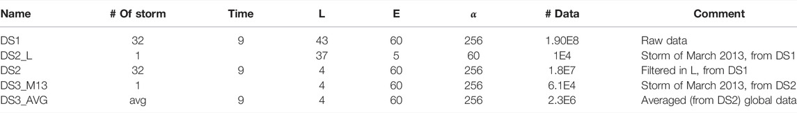
TABLE 1. List and properties of the various datasets in use.
In this article, we first restrain the dataset by choosing values of L at a few discrete points L = 2, 3, 4 and 5, which gives around 18 million data. Five L-shells are enough to be representative of the general behavior of the diffusion coefficients, i.e., the spread of the cyclotron component over pitch angle, in order to first focus on the reduction in (E, α) at fixed L. This dataset is called DS2; see Table 1. The reduction method in (E, α) is then directly extended to a finer grid in L in the case of the 32 storms global model (cf. Section 2.1.4).
2.1.3 Dataset for the Storm of March 2013
The dynamics of the electron radiation belts during the month of March 2013 have been subject to much attention (e.g., [3,11,12,16,62,63]). The storm of March 1, 2013, is associated with a high-speed solar wind stream that created strong erosion of the plasmasphere and resulted in outer belt flux dropout events. The storm was followed by enhancements of relativistic electrons in the slot region and outer belt during the 3 days. An extended period of quiet solar wind conditions persisted then for the 11 next days, with the plasmasphere expanding outward to L ∼ 5.5. For this event, Ripoll et al. [11] showed the electron depletion in both the slot region and the outer belt was caused by pitch angle scattering from whistler mode hiss waves. Ripoll et al. [16] extended the demonstration to a global analysis of the 3D (L, E, α) structure of the radiation belts during the quiet times from March 4–15 and compared the output of event-driven Fokker-Planck simulations to pitch angle-resolved Van Allen Probes flux observations with good agreement.
In this section, we focus on the specific storm of March 1, 2013, and we use the event-driven diffusion coefficients database that was generated for the studies of Ripoll et al. [16]. Specific parameters of the diffusion coefficients are given there and not recalled here. These coefficients use the local wave and data parameters and as such can contain the noise and the variability of the measurements. But since the expression of the diffusion coefficients is made of the combination of tractable mathematical expressions, with some oscillating Bessel functions, and a series of summation (over the harmonics) and integration (over both frequency and wave normal angle) (e.g., Albert [48]), the database ends up being quite smooth and not too noisy. This will be a key property of the data for choosing or developing an adapted machine learning method. In addition, the diffusion coefficients are also time-averaged from March 1 to March 5 in order to provide a single diffusion coefficient defined for L-shell L, energy E, and pitch angle α. This time-averaging made over 5 days (representing 15 temporal bins of 8-h averaged together) produces smoothed data, i.e., a regularized dataset, which may otherwise be more variable over time and less smooth (e.g., Figure 5 in Ripoll et al. [12]). As we average, we mix different geomagnetic conditions and create a mean diffusion coefficient for that 5-days event. The time-averaging is only done in this section and will not be done in the HSS section in which we will keep time as another variable. Absence of noise and regularized data make our problem specific. On the contrary, in general, data have uncertainties coming either from our partial knowledge of the variables, or from data variability. In our case, we can have experimental and simulation uncertainties. In such cases, machine learning models have to avoid over-fitting, by not being too close to the data during training. In this article, regularization of data was such that over-fitting was not an issue.
For this storm, we use 4 positions, 60 energies, 256 pitch-angles, i.e., 61440 data points for (L, E, α, Dαα) listed as DS3_M13 in Table 1. We extract a subset of DS3_M13 that is composed of 84 pitch angles and 60 energies bins, thus 20,160 data points, listed as TRAIN_M13 in Table 2. This dataset is used for training and calibrating the internal parameters of the various machine learning models using cross-validation.
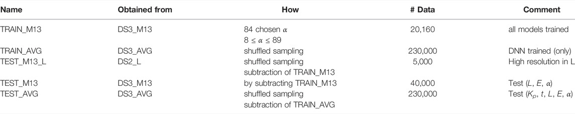
TABLE 2. The datasets used for training (2 first rows) and testing (3 last rows). Test data are obtained by subtracting the training and validation datasets from the data, and all points that are outside the bounds of these training and validation datasets, so as to avoid extrapolation in the test.
To evaluate the ability of the machine learning models that we trained on the TRAIN_M13 dataset, to generalize on new data, we consider 2 test datasets; see Table 2. The first dataset TEST_M13_L contains more values in the L input. The model was trained with 4 L-values (L = 2, 3, 4, 5), and here we have 37 values from L = 2 to L = 5: thus we test the interpolation between the discretization used during the training in the case of a very low resolution. The other test dataset (TEST_M13) has full resolution in angles and energies, but the same resolution in L. The test datasets have no intersection with the training dataset. We have also excluded all extrapolation points (with an exception for Kp in Section 3.2.3), signifying that we bound the test datasets with the bounds of the corresponding training datasets, when evaluating errors.
2.1.4 Dataset for the 32 HSS Storms
In this section, we extend massively the previous problem from 1 storm to 32 storms. We choose storms all among the same family of storms called high-speed streams (HSS) so that we can compare them together, characterize the differences, and compute relevant statistics. By doing so, we try to optimize our chances to address similar physical processes and their spatio-temporal timescales. These 32 HSS were each identified in Turner et al. [43] between September 2012 and December 2016 (listed in Table 3). Each storm is observed at various MLT positions, changing with the Probes orbit. When Van Allen Probe B is at its apogee, the corresponding MLT is reported in the right column of Table 3. This MLT corresponds roughly to the most observed MLTs from L above ∼ 4 up to L ∼ 6. The 32 storms are such that we have 10 events observed from the night side (MLT = 21–3), 11 from the dusk side (MLT = 15–21), 4 from the day side (MLT = 9–15), and 7 from the dawn side (MLT = 3–9). Some of the differences we found may be attributed to MLT variations, though keep in mind that the statistical MLT-rescaling of the wave power makes the coefficients valid and comparable over all MLTs.
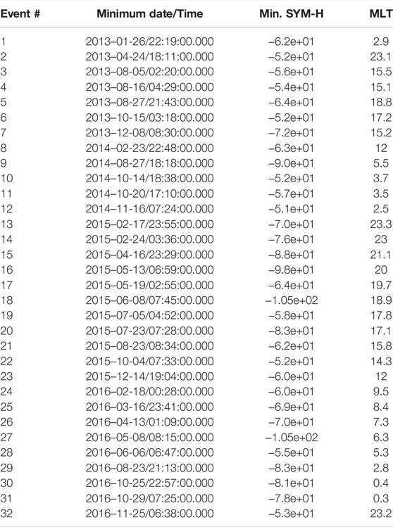
TABLE 3. From left to right: number, Date and time, minimum Sym-H index (i.e., high resolution Dst index) and MLT of the apogee of probe B of the Van Allen Probes for each of the 32 high speed streams between September 2012 and December 2016 of this study (reported from the selection of the HSS events of Turner et al. [2019]).
For each observed storm, we extract wave and plasma data from the Van Allen Probes during 3 days, every 8 h, which gives 9 intervals of 8 h. The timescale of 3 days is representative of the HSS main and recovery phases seen in Turner et al. [43]. The measurements are used as inputs in the simulations of the quasi-linear pitch-angle diffusion coefficients Ripoll et al. [16] outputted at this rate, producing the full database DS1.
For each storm and for a given time bin, we have a discretized grid (L, E, α) of the diffusion coefficient. For each temporal bin, we store the Kp index (itself averaged over the 8 h bin duration). The Kp-index is the global geomagnetic activity index that is based on 3-h measurements from ground-based magnetometers around the world. The Kp-index ranges from 0 (very little geomagnetic activity) to 9 (extreme geomagnetic storms). The Kp index is largely used in the radiation belt models as a main parameter of wave models driving radiation belt simulations (e.g., Cervantes et al. [61]; Sicard-Piet et al. [18]; Wang et al. [41]). Here, it works as a measure of the storm strength at a given time. We define averages per Kp index and regroup the diffusion coefficients per Kp. The Kp index then becomes the 5th variable, which was first meant to replace the time variable, as any Kp average model, but we will explain later that time was nevertheless kept. As such, we have 18 million data points in (t, Kp, L, E, α, Dαα), which gives data set DS2.
We build a first set of averaged diffusion coefficients by considering all the 32 storms, each defined at 9 temporal bins, which now define 9 epoch times. For a given temporal bin j = 1‥9, for a given Kp = 0, … 6, we average Dαα(L, E, α) over all the storms. We obtained this way 2,300 000 data points, listed as DS3_AVG in Table 1. The model is defined for (t, Kp, L, E, α). Averages are made at fixed Kp for each tj. (If we were averaging without binning by the Kp index, we would produce a superposed epoch model of diffusion coefficients.) Here, the approach produces a superposed epoch model of the diffusion coefficient, further binned by Kp. Such an approach allows the diffusion coefficients to evolve in time, keeping within its origins ambient properties that are consistent with each other, always keeping the coupling between the electron plasma density and all wave properties. This approach is different from making a superposed epoch model of the wave properties of HSS and computing afterwards a single diffusion coefficient from them. The latter approach has low numerical cost but neglects correlations between all the properties of the ambient domain and, therefore, introduces some error (e.g., Ripoll et al. [17]). From a machine learning perspective, the Kp averaging helps produce smoothed data, acting as a regularization of the solution that makes the solution less fluctuating, i.e., less noisy from a ML-perspective, similarly to the temporally-averaged data of the March 2013 storm (as discussed in section 2.1.3). From DS3_AVG, we train on 10% of the data, listed as TRAIN_AVG in Table 2. All datasets are described in Table 1, training and validation datasets in Table 2 (2 first rows), and test datasets in Table 2 (3 last rows).
2.2 Machine Learning Methods
In this section we briefly describe the several statistical and machine learning methods that we used to build the various models of this study. We considered methods based on local evaluation (k-nearest neighbors and kernel regression), tree-based methods (regression tree, bagging and random forest), neural networks, and function approximations (Radial basis and splines). All are nonparametric so that we make no assumption about the distribution of the data. A detailed description of all these machine learning methods can be found in Hastie et al. [64], and complementary information about neural networks can be found in Géron [65]and Goodfellow et al. [66].
2.2.1 K-Nearest Neighbors
A key idea in many supervised machine learning methods is to think that the targets associated to nearby inputs should be close to each other. Based on this idea, to predict the target of any new input data points, it is reasonable to look at the target values of their surrounding neighbors. This is the whole framework of k-nearest neighbors machine learning method which predicts the target of new input data by averaging the target values of its k-nearest neighbors, measured using the Euclidean distance (see, for example, Fix and Hodges [67]; Altman [68] and Hastie et al. [64]). The number of nearest neighbors k is the key parameter and it is very crucial to tune it using cross-validation technique described in the following. On one hand, if k is too large, a large number of observations, among which not very representative ones, contribute to the prediction, resulting in too rough predictions. On the other hand, if k is too small, the prediction is made relying only on a small number of neighbors of the query point, resulting in high variance.
2.2.2 Kernel Regression
The k-nearest neighbors procedure may be modified to obtain a smoother method, which gives more weight to the closest points and less to the furthest: instead of specifying a number of neighbors, the neighborhood is defined according to a distance notion, via a kernel function, that is a function K: Rd → R+, such that K(x) = L (‖x‖), where x↦L(x) is nonincreasing. More specifically, a prediction
where the kernel Kh is defined by Kh(x) = K (x/h), with h the bandwidth of the kernel, and (Xi, Yi), i = 1, 2, … , n, denotes the input-output training data. Here, a Gaussian kernel has been considered:
for some σ > 0. For more about the method see, for example, Nadaraya [69] and Watson [70].
2.2.3 Regression Tree
Another nonparametric model commonly used in regression problems is regression tree. It is an iterative partitioning algorithm aiming at each step to split the input space along the value of a chosen predictor and threshold, minimizing the target variance on both parts of the split (see Breiman et al. [71]). Growing a tree is equivalent to partitioning the input space into smaller and smaller regions containing lesser and lesser points. The prediction of a new data point is the average target values of the points falling into the same region as the query point. Growing a single deep depth tree on the training data (small terminal nodes or small region) will most likely lead to over-fitting. Moreover, a deep depth tree can be very sensitive (high variance) meaning that a small change in splitting the training data can result in a very different structure of the tree. It is then important to tune the depth of the tree, which is the key parameter. This may be done using cross validation technique.
2.2.4 Bagging
The aim of this method is to reduce the variance of regression trees by introducing bootstrap samples from the training data. A regression tree is grown on each bootstrap sample, and the final prediction is the average of the predictions of all the trees (see Breiman [72]). This method is shown to be significantly more accurate in generalization capability. The parameters of the method are the number and the depth of the trees to be constructed on the bootstrap samples.
2.2.5 Random Forest
As each tree in Bagging method is constructed using a bootstrap sample of the training data, the constructed trees are likely to be quite correlated. Random forests have been proposed to enhance reduction of the variance. They aim at producing uncorrelated trees by randomly selecting only a subset of features at each split in the process of growing the trees. In regression problems, the size of the set of features to be randomly selected at each split is usually taken around
2.2.6 Neural Networks (DNN)
We use feed-forward neural networks as a regression model. A neuron is the composition of a nonlinear function (here we use Relu(x) = max (0, x)) and a linear function. All inputs enter the N1 neurons of the first layer. Then each neuron gives an output, and each output connects to the N2 neurons of the second layer. We do the same for all the layers (the number of such layers is the depth of the network), and we end with a layer of one neuron (because we have one output, the pitch-angle diffusion coefficient), which has no nonlinear function. It has been shown [75] that any reasonable function may be approximated by one layer of neurons, but the practice has shown that it is better to go deep, which means to use a lot of layers (which entails a lot of composition of nonlinear functions, that is to say a lot of interactions between the inputs).
The coefficients of the linear functions of all the neurons are tuned by an optimization algorithm. This phase is called the training. We use a variant of the stochastic gradient descent method (the Adam optimizer) to minimize the mean square error between data and predictions.
Neural networks are accurate for regression problems and extend well to a huge dataset or to high dimension problems. One difficulty is that such a model involves a lot of hyperparameters, and many combinations of these hyperparameters may give low accuracy results. For example, we have to choose the architecture (number of layers and neurons per layer), the initialization of the linear coefficients, the optimization algorithm, the number of epochs (iterations of the algorithm) and batches (splitting of the data to calculate gradients in the stochastic gradient descent). In order to optimize these choices, an original specificity of our DNN model is to use a data-driven method for selecting all these hyperparameters [76,77]. It uses random forest methods (which has a few hyperparameters, see Section 2.2.5) and a mapping between the obtained trees and the architecture of an ensemble of neural networks. We obtain this way accurate neural networks with only 2 hyperparameters, the depth and the number of trees. When we obtain this accurate network, we may search for higher accuracy by playing with other hyperparameters that were fixed in the first step.
2.2.7 Thin Plate Spline
Thin plate splines, introduced by [78], may be seen as an extension of cubic smoothing splines to the multivariate case [79]. In the one-dimensional case, cubic smoothing splines are used to construct new points within the boundaries of a set of observations. They are fitted using a penalized least squares criterion, with the penalty based on the second derivative. The interpolation function consists of several piecewise cubic polynomials. Fitting low-degree polynomials to small subsets of values instead of fitting a single high-degree polynomial to all data allows us to avoid the Runge phenomenon, that is, oscillation between points occurring with high-degree polynomials. Cubic smoothing splines are widely used since they are easy to implement and the resulting curve seems very smooth. More specifically, if we observe data (X1, Y1), …, (Xn, Yn), the quantity to be minimized is defined by
where Y is the vector of observed outputs Y1, … , Yn and f = (f (X1), …, f (Xn)). In the general case, the main part of the criterion remains the same, but the shape of the penalty is far more involved, based on several partial derivatives. Thin plate splines are given as functions f minimizing
where
and the factor λ drives the weight on the penalty. Here, m is such that 2m − d > 0, and the νi’s are nonnegative integers such that
2.2.8 Radial Basis Function Interpolation
A Radial Basis Function (RBF) is a function that depends only on the distance between the input and a predetermined fixed point, called a node. We can use RBF as a basis for an interpolator in the form:
where N is the number of nodes, hi are unknown coefficients, and ϕi(x) = ‖x − xi‖, with xi the coordinates of the ith node. Here, we use all the points in the training set as nodes. The training consists in finding the values of the coefficients hi by imposing that the interpolant passes exactly through the targets in the training set, that is f (xi) = Y(xi). This amounts to solve the linear system
2.2.9 Cross-Validation
Each method depends on some key smoothness parameters (usually called hyperparameters) that need to be tuned properly to get a good performance. This is done via cross-validation. K-fold cross-validation consists of breaking down the training data into K folds {Fk: k = 1, 2, … , K}, and for a given candidate parameter, the corresponding model is constructed using as training set the K − 1 folds where the remaining fold is treated as a validation dataset. Thus, for a given value of parameter β, the corresponding model f is trained K times (K different combination of K − 1 folds choosing from the total K folds). We then measure the performance of f at the choice of parameter β using the cross-validation error defined by
In the particular case where each data subset only contains one single observation, the method is called leave-one-out cross validation.
Roughly speaking, this provides the average performance of f associated with the parameter β on K different unseen folds of the training data. The parameter
For k-nearest neighbors, kernel regression, regression tree, bagging, and random forest, a 10-fold cross validation was used. For thin plate splines, the penalty coefficient is estimated through generalized cross validation, which may be regarded as an approximation to leave-one-out. For the neural networks, the training data set was randomly cut in 3 parts: 80% for the training, 10% for checking over-fitting during the training, and 10% for selecting the final network. After that hyperparameters selection, all results presented in this article are obtained on a huge separated test dataset, as showed in Table 2.
2.2.10 Complexity of the Training and Computational Time
Training phases are very different between all methods: for KNN there is only a search over the existing space of data. In tree-based methods the training corresponds to the construction of the trees. In DNN the training corresponds to the search for the weighting factors in the interconnections. All training phases agreed in the choice of the hyperparameters: as data have no uncertainties, and are somehow regularized, our methods have to fit to the training data. This means for tree-based methods to grow deep trees (one point in the final node), to be very localized for the k-nearest neighbors method (K = 2) and kernel regression, and to go deep with neural networks, with many epochs. Ensemble methods do not need to be pushed too far: for tree-based methods, we used 100 trees, and for neural networks, we averaged the outputs of around 5 networks. Moreover, thin plate splines are specifically dedicated to interpolation.
Even if the methods depend on the choice of hyperparameters, we can still say that the cpu-cost of training is about a minute for both regression tree and k-nearest neighbours, about 10 min for bagging and random forests, and 2 h for neural networks, with each method using around 20,000 data. Predictions are fast for all methods, meaning they take a few seconds maximum for 60,000 data.
3 Results
3.1 Results for the Storm of March 2013
The numerical results reported in the following tables and figures present an analysis of the distribution of the errors:
The TEST_M13 test data set is detailed in pitch-angles and energies but contains only 4 discrete L-shells values (L = 2, 3, 4, 5). The TEST_M13_L data set is however detailed in L and contains L-shell values regularly spaced from L = 1.6 to L = 5.2 by 0.1 step (37 values) and a few angles and energies values. These datasets are sampled on a grid and there is no uncertainty on the points. Hence, as already mentioned, all models are trained until reaching a small error value on the training data set. We first start by addressing the error with respect to the (E,α) resolved grids and then on the grid resolved in L-shell.
3.1.1 Variation With (E, α)
Results in Table 4 show that the Spline, the RBF, and the DNN models outperform with the lowest mean and maximal absolute error. We also observe that the Spline and the RBF have very low medians which show that they are very good on many samples, but have also many outliers, with big error. The DNN shows a median error close to the mean.
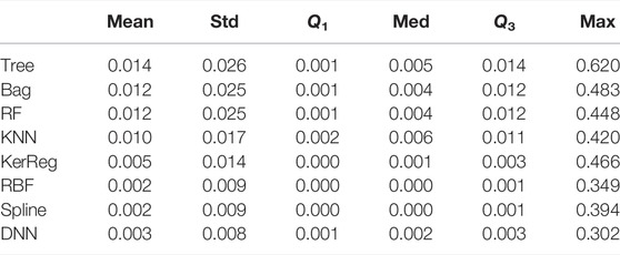
TABLE 4. Performances of all the methods trained on TRAIN_M13 and tested on TEST_M13. We consider the absolute error |ei| and report the mean error, standard deviation, first quartile, median error, third quartile, and maximal error.
The violin plots in the top panel of Figure 1 complement well Table 4 in showing that the underlying statistical distributions of the errors differ from one method to the other. DNN, Splines, and RBF have the most concentrated distributions at low errors, especially both the Splines and RBF methods, with spline with a mode around the mean and RBF with a mode around the median. As seen on Table 4 with the maximal error, this hides more outliers with Splines and RBF than with DNN.
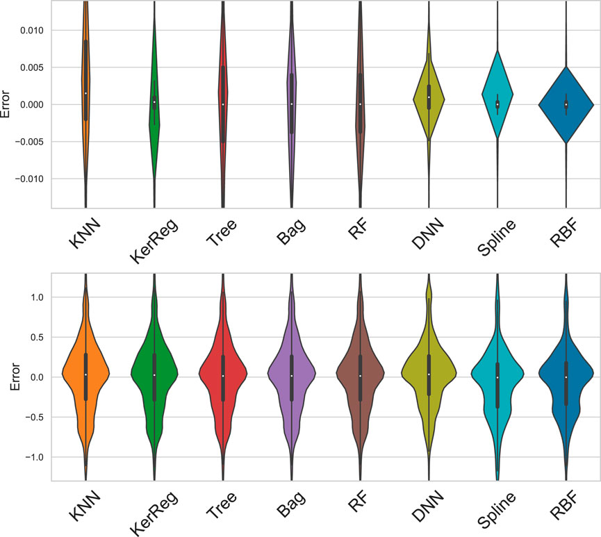
FIGURE 1. Violinplots of error
These results start to exhibit two main families of methods: on one hand the Tree family (Tree, Bag, RF) with KNN and KerReg, and on the other the RBF, spline, and DNN methods.
In order to get insights on the differences and similarities between the machine learning models, we now compute the correlation between the errors provided by a couple of different models. The correlation errors are given in Figure 2 for TEST_M13, on the left. First, Figure 2 confirms the 3 methods (Tree, Bag, RF) fall into the same family, with high correlation
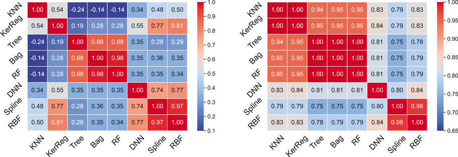
FIGURE 2. Correlations of error
Finally, this study was also conducted at low resolution with 13 energies and 14 pitch angle resolution, representing 728 data points (results not shown). Although some small changes of behavior either within or among the methods were visible, the conclusions were similar, for an admissible accuracy of the diffusion coefficients. Machine learning methods can thus be used to find an optimum between accuracy and resolution, reducing this way the high original cost of computation of the diffusion coefficients.
3.1.2 Variation With L-Shell
In this section, we consider each method for its ability to capture the L-shell dependence. It should be noticed that all methods have been trained on a very crude L-shell resolution, containing 5 L-shells only, and that they are now tested against data fully resolved in L-shell. This test is therefore very challenging and only made to gain insight on the properties of the ML methods. If a full model in (L, E, α) had to be generated (cf. Section 3.2), the approach would be to train on a higher L-shell resolution and not to interpolate a low resolution grid.
Table 5 presents the main error global metrics, with errors much higher than in the previous section due to the initially low L-shell resolution. The mean error gradually decays from the Forest tree family to DNN (from top to bottom). However, the median error remains more similar, still decaying from top to bottom. Best performances are always obtained from either the Spline, the RBF, or the DNN method.
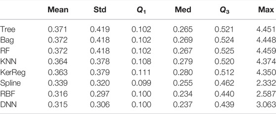
TABLE 5. Performances of all the methods trained on TRAIN_M13 and tested on TEST_M13_L. We consider the absolute error |ei| and report the mean error, standard deviation, first quartile, median error, third quartile, and maximal error.
Violin plots of the distributions of errors have been generated (on the bottom of Figure 1). All the distributions are found very alike in their global shape, with only subtle differences. Some methods show two or even three modes which appear as peculiar oscillations on the edge of the distribution.
Figure 2 (on the right) shows the error correlation among the couples of models for the test with respect to L-shell. The main families previously mentioned remain, this time with KNN and KerReg performing similarly to the Forrest tree family. Based on these results and the one of the previous section, all 5 models (Tree, Bag, RF, KNN, KerReg) are regrouped into the same family.
We finalize this series of tests by Figure 3, in which we compare the forest tree family (represented by the RF method), the spline method, and the DNN method for a few selected (E, α) but resolved in L-shell. The training phase being done at L = 2, 3, 4, 5 (indicated by vertical bars), we see all models provide an exact answer at these points. Everything in between these points is modeled (orange line plots) and compared with the exact solution (blue crosses). The random forest model plotted in Figure 3 (left) uses constant approximation around the training points so that the approximation is made by step functions and is extremely crude. It is the same for tree-based methods, k-nearest neighbor, and kernel regression (not shown). The spline method does much better in Figure 3 (center), but cannot approximate brutal variations, as for radial basis model (not shown). The DNN method in Figure 3 (right) seems to us the most capable for this difficult exercise, which confirms the global metrics of Table 5.
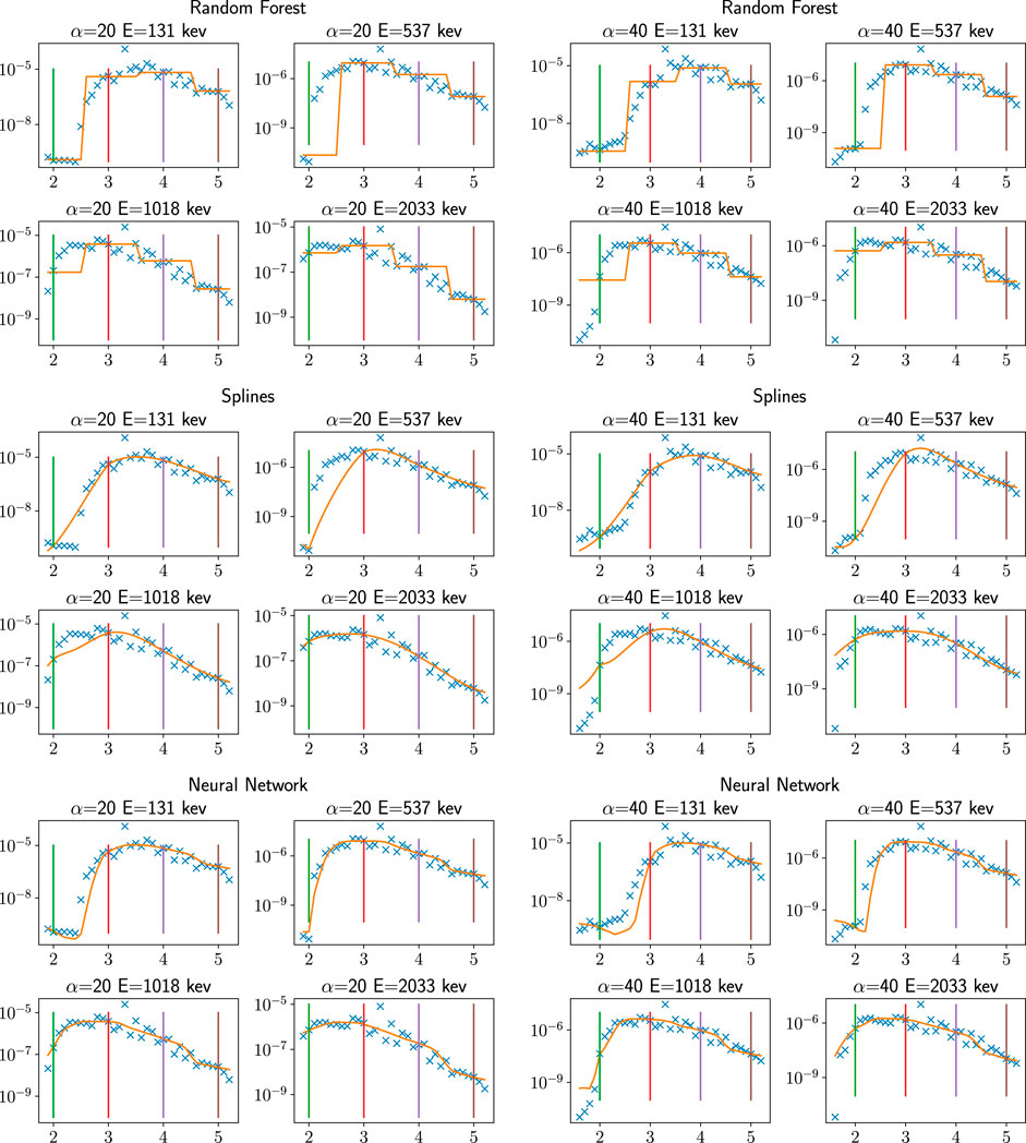
FIGURE 3. Machine learning pitch angle diffusion coefficients (Dαα(L) in s−1 on the Y-axis) for the March 2013 storm plotted in orange color versus L-shell (X-axis) for various pitch-angles (20° and 40°) and energies (131, 537, 1,018, 2,033 Kev) computed from (top) random forest, (center) thin plate spline, (bottom) neural network. The blue dots are the reference original diffusion coefficients (points of TEST_M13_L which were not used in the training and testing phase). Vertical lines represent the location of the training data of TRAIN_M13 (L = 2, 3, 4, 5). These plots were made with methods that were trained on a subset of TRAIN_M13: we used fewer points in energy and pitch-angles.
We conclude that without any prior assumption on a physical phenomenon and on the database, it is difficult to advise the use of a particular machine learning model. One main reason is the data used to train the model have a big influence on the model performance, which makes it hard to generalize the capabilities of a given model. Here, we believe the different series of tests and comparisons are explicit enough to conclude that the DNN method is a good candidate to perform the rest of the study and to generate a more global model.
3.2 Results for the Global Model of Pitch Angle Diffusion During HSS Storms
In this section, we use the data from 32 storms in order to build a database of statistical event-driven diffusion coefficients that is embedded within a machine learning model for facilitating its use. The method relies on constructing first an averaged model and then using the deep neural network (DNN) previously selected to learn and output the solution of the averaged model. As in the previous sections, we will see the machine learning model does not entail any issue to interpolate and reproduce the averaged model. Questions arise more about the physical choices we make to build the averaged model (cf. discussion below and in Section 4.1). Interestingly, the machine learning model was of great help for the various investigations we conducted. As the training step was quite fast (based on the knowledge acquired during the March 2013 storm study), we could test different ways of manipulating and averaging the data when iterating to choose how to best parametrize the statistical model. Another strength of the machine learning approach is the simplicity of performing comparisons with the model since it delivers continuous maps of the solution with a simple numerical subroutine able to output a 5 to 6 dimensions solution. On the contrary, manipulating directly the database and using discrete points is very constraining. It can also be source of direct errors or interpretation errors when it is a given plotting software (e.g., Python subroutines) that carries intrinsic ad-hoc interpolation with integrated smoothing procedures.
3.2.1 Training the DNN Global Model
The data used to generate the global model is DS3_AVG described in Section 2.1.4 with 2.3e6 data points. We then use TRAIN_AVG (2.3e5 data points), unless specified differently for training and validation, and TEST_AVG (2.3e5 data points) for test.
The training of the global model Dαα(Kp, t, L, E, α) was not harder than the model previously trained for the storm of March 2013 in Section 3.1. The two more dimensions of the input space entailed a larger neural network. The bigger amount of data (from 20,000 to 230,000) caused a longer training. Generating the whole model took a few hours of computation on a standard computer. For comparison the simple generation of a mean model, without machine learning and performing only means throughout the whole database, took a few days on the same computer. Again for comparison, computing 19.3M diffusion coefficients for around 10-days event takes around 15,600 h spread over 1,300 processors on a CEA massively parallel supercomputer [17]. This brings another advantage of machine learning methods to be able to manipulate simply and at low cost a large database, with the possibility to operate on them basic statistical operations useful for the understanding of the database.
In Figure 4 (left), we represent the mean average error (MAE), the mean square error (MSE), and one minus the explained variance score (EVS) computed when the model is evaluated against the TEST_AVG test dataset (230,000 data not used during the training phase performed with the TRAIN_AVG dataset). Because the dataset contains little noise, we can train neural networks going deep, with depths of the network going from 6 to 11 hidden layers on the x-axis. We see an optimum of low values of the three metrics is found for a depth of 9.

FIGURE 4. Errors calculated on the dataset TEST_AVG are plotted for different DNN models, with various depth on the left, and various sizes of training dataset on the middle. On the left, models are trained on 10% of the data, meaning around 230,000 data. On the middle, dot lines with circles are for a model of depth 8, and continuous lines with crosses for a model of depth 9. In blue, we plot the Mean Average Error, in red the Mean Square Error, and in black one minus the Explained Variance Score. On the right, the loss function (MSE) is plotted during the training, evaluated on the training dataset, and on the validation dataset. We see at the end that we make more often evaluations of these errors, and the training stops selecting the more accurate model in the last epochs. Note that this loss may not be compared with anything in this article, as it is given on scaled data.
The same three quantities are plotted in Figure 4 (center) using different sizes of training dataset (from 1 to 15% of the TRAIN_AVG dataset), with DNN of depth 8 or 9. From these results, we selected the neural network of depth 9 trained with 10% of the data. As over-fitting is not an issue here, we could reach better accuracy by taking a more important capacity for the model, or just by taking more epochs as discussed next. This is not obvious on Figure 4 as with a higher depth, error is growing (after depth 9), but it is possible to be more accurate by varying all hyper-parameters. However, we have also seen that the loss of accuracy due to the DNN model is less the issue than the loss of accuracy caused by an averaged statistical approach (cf. discussion in Section 3.2.2).
Figure 4 (right) represents the loss function during the training and the validation phases of the model of depth 9 over 10% of the data. The loss function is the minimal MSE computed over all the data and evolving according to the epoch number, which represents the number of cycles the data are used in a training or validation step. After 900 epochs, we evaluate more often the loss function, because we stop at the best loss value obtained on the validation dataset.
3.2.2 Accuracy of the DNN Global Model
We present in Figure 5 the obtained deep neural network (DNN) global model of diffusion coefficients, which is plotted in green for two of the 32 selected storms. We choose for illustration storm 8 (3 top rows) as event-driven and average diffusion coefficients agree quite well and storm 5 because the opposite occurs. We also plot in red the average model, which represents what the DNN model (in green) has to reproduce. Each storm is decomposed in 9 times with its Kp index history (as shown in the bottom panel of Figure 5) and the DNN model is played for the (t,Kp(t)) sequence of this storm. Results are presented at L = 3, 4, 5. We omit L = 2 for the sake of brevity since diffusion is limited to high energy (see discussion in Section 3.2.3 and Figure 6 top row).
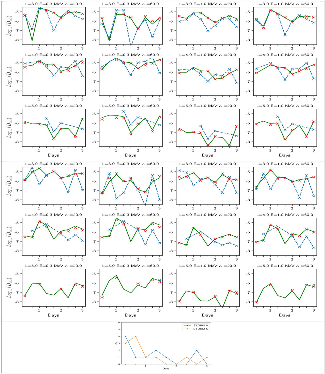
FIGURE 5. Pitch angle diffusion coefficients for (1–3 rows) storms 8 and (4–6 rows) storm 5. The first 6 panels show historic pitch-angle diffusion coefficient's at different (L, E, α) values, with (blue crosses and lines) the raw data of event-driven coefficients (red crosses) the averaged data (on the 32 storms at given (Kp, t, L, E, α)), and (green lines) the DNN model. The average data (in red) and the DNN model (in green) (trained on a subset of the average model) are run from the Kp(t) sequence of each storm plotted at the bottom panel for each of the 9 temporal bins. The good agreement between red crosses and the green line shows the success of the DNN model at matching its target. Both capture levels and variations, but are not very accurate compared with the event-driven diffusion reference values in blue, showing the limits of a mean model.
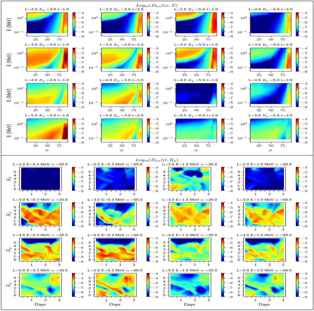
FIGURE 6. The DNN model of (Dαα) (Log10 of s−1) in the (top) (α, E) plane at fixed (L, Kp, t) and (bottom) (t, Kp) plane at fixed (L, E, α).
As we can see for storm 8, the DNN model is very close to the average model, as it should be, as soon as the intrinsic interpolation rules of the model have been learnt well. This is confirmed for storm 5 in Figure 5, which ends our demonstration that the restitution of the DNN model is accurate. Figures like Figure 5 (3 top rows) have been generated for each of the 32 HSS storms (not shown), which allows us to reach an individual view of each of them and confirm the accuracy of the DNN approach. This occurs at all L-shells used to derive the DNN model.
We now use the DNN mean model to analyze how mean coefficients behave compared with individual ones. An important physical question arising in space weather forecasting is the ability of an average model (e.g., from the DNN approach or directly from averaged data) to precisely predict the history of the diffusion during the storm. We thus compare in Figure 5 the DNN statistical model (in green) with the event-driven diffusion coefficients (blue cross). We find the average procedure captures quite well the global variations of the pitch-angle diffusion coefficient in general for storm 8 but fails by a significant factor at various (t,L,E,α). This way we start to enlighten the difference between an event-driven approach and a mean approach thanks to the machine learning interface. We see for instance an interesting strong departure at (L = 3, E = 0.3 MeV, α =60°, t= 1.6 days) for storm 8 between both the average models (green and red) and the event driven model (blue). Readers will understand in the next section (based on Figure 6 top, left) that α =60° falls right at the sharp edge between significant diffusion of the cyclotron harmonics and absence of diffusion for E = 0.3 MeV electrons at L = 3. Both average models capture thus (on average) significant diffusion while for storm 8 at t = 1.6 days the diffusion is negligible, causing an error by more than 2 orders of magnitude. Note that all models agree for the time before (t = 1.3) and after (t = 2.). This is likely due to the particularity of the wave conditions at t = 1.6. Conversely, Storm 5 (fourth to sixth rows of Figure 5) is an example of the opposite, with a storm for which the diffusion coefficient behavior (in blue) is opposite to the mean behavior (red and green). The error between the average model and the event-driven coefficient is often large, up to 2 orders of magnitude. We see the same feature as for storm 8 at L = 3, E = 0.3 MeV, α =60. Large errors at L = 2 (not shown) for 1 MeV electrons are also likely due to the average model missing the particularity of a local increase of diffusion close to a strong gradient region. At L = 5, we see the absence of the event-driven coefficients for that case, except for the point at the latest time, at t = 3 days. This can be due to the plasmasphere that has not recovered up to L = 5 during the first 2.6 days and the absence of hiss waves, to the absence of measurements for that event, or both. The average model returns low diffusion most of the time (below 10–6), except for E = 0.3 MeV and α = 60.
3.2.3 Exploring the DNN Global Model
We now explore and discuss the main physical characteristics of the statistical mean model of pitch angle diffusion coefficients for HSS storms thanks to the DNN encapsulation.
At fixed (t, Kp), we see pitch angle diffusion occurs at lower energy as L increases in Figure 6 (four top rows). At low L-shell (L < 3), we see a wide region of negligible diffusion in the (E, α) plane. This region of no interaction is due to the first cyclotron harmonic that does not reach pitch angles higher than the loss cone pitch angle [12]. The DNN model has thus to learn more very low values at low L-shell. This absence of pitch angle diffusion explains why electrons are not scattered out by hiss waves and remain trapped at low L-shell in the inner belt. With the storms compressing the plasmapause, the model allows us to see better if there is more effect at low L-shell. Figure 6 shows diffusion is non negligible above ≃ 700 keV at L = 2 and becomes stronger for active conditions (Kp = 5 at t = 1, first row and third column) when hiss power is localized deep inside the plasmasphere. For Landau diffusion (pitch angle above 80°) of electron below 300 keV, we notice a transition between significant Landau diffusion and an absence of diffusion for the highest pitch angle (above 85°) at Kp = 3 and t = 1 day, which is likely the DNN model reaching its limit. We will come back on this negative feature in the next section.
At higher L shell (L ≥ 3) and fixed energy, the minimum pitch angle diffusion occurs between first cyclotron harmonic and the Landau (n = 0) harmonic (e.g., between α = 75 at L = 4, E = 200 keV, Kp =3, and t = 1). At fixed L shell, the maximal pitch angle diffusion from cyclotron harmonics occurs at higher energy as pitch angle increases. The sharp gradients that occur for given (L, E, α) values in the region of transition between Landau and cyclotron resonance reduces as L increases, but it remains a region of possible errors as commented in the previous section for L = 3, E = 0.3 MeV, and α =60 in the third row of Figure 5.
One could wonder why the diffusion at L = 4 and Kp = 5 is negligible at t = 1. This is due to the fact that for such active condition the center of the plasmasphere where hiss is dominant (e.g.,[39]) is located at lower L-shell, while L = 4 is in a region of minimal hiss activity, likely in the vicinity of the plasmapause (if beyond, the wave would not be defined and the diffusion would be null). Further investigation in Section 4.1 and Figure 7 will show that there exists only once case of storm having Kp = 5 and t = 1 so that the mean DNN model has learnt the solution shown in Figure 6 (two top rows and third column) from a single storm event. As interesting is the absence of storms with Kp = 5 at t = 2 days (cf. Figure 7) so that the model is extrapolating with respect to Kp in Figure 6(two top rows and fourth column). At t = 2 days, the model statistically predicts some waves with some power due to the fact that likely the plasmasphere has often recovered to above L = 4 at that time, bringing some hiss power. We understand the model could learn such behavior from the data. But would that be occurring in reality if Kp was still as high as Kp = 5 on the second day of a HSS storm? We cannot tell from the current data.
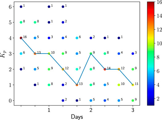
FIGURE 7. Numbers of storms that have Kp and t values. The number of storms in each (t,Kp) bin is written and colored and represents the number of elements averaged together per (t,Kp).
Looking at fixed (L, E, α) values in Figure 6 (two bottom rows), we see any storm can be represented by its evolving path in the (t, Kp) space, with possibly great differences from one time to another although each storm belongs to the same kind. There is a large variability of pitch angle diffusion coefficients with respect to time looking at a horizontal line of fixed Kp. The diversity of the wave and plasma conditions leads to decay rates varying by orders of magnitude and although the Kp indices are the same. This contributes to explain why storms can be so different from one event to the other (e.g., [80]). This brings the question of the time resolution of Kp (here 8 h) and the pertinence of this index when considered as the only parameter of geomagnetic activity. The MLT location of all the observations could also explain the differences. Time plays a crucial role in the solution (cf. the discussion on the interpretation of time in section 4.1), while diffusion coefficients do not depend on time in most common space weather simulations (e.g., [61]) in which only Kp remains in both the wave models and the diffusion coefficients (sometime even in the absence of the L-shell dependence (e.g., [81]). The variability of the wave parameters calls for the use of at least two geomagnetic indices or one geomagnetic index and another relevant parameter (here, directly time).
For a given (L,E), we see in Figure 6 (two bottom rows) the pattern and shape in at fixed (E, α) is roughly conserved while the levels changes. This is true because the solution is presented at not too low L-shell (L ≤ 3) such that the region of minimal diffusion at moderately high pitch angle between the Landau and cyclotron resonance is narrower than at lower L-shell (Ripoll et al. [12]). Nevertheless, there exist regions in the (E, α) with shapes and variations that differ from the main general trend, as, for instance, illustrated in Figure 6 (two top rows).
Further exploration of pitch angle diffusion during HSS events is discussed in Ripoll et al. [82] and, in particular, the variability of diffusion within a same Kp index bin. This exploration of the DNN model leads us to look at which diffusion is predicted by the model during sustained HSS yet unobserved.
4 Discussion
4.1 Average vs. Event-Driven Models
The number of storms for each activity (Kp, t) is represented in Figure 7. The specificity of storms (e.g., [80]) appears clearly with a few or none events for some combinations of (Kp, t). For instance, there is no HSS storm that has a mean Kp = 0 within the 8 first hours. However, there is one HSS storm (over 32) for which Kp = 1 occurs within the second period of 8 h of the storm. In great majority, HSS storms have a mean Kp index of Kp = 4 during the first 8 h. 2.6 days after the storm 70% of HSS storms (22 over 32) have Kp between 1 and 2, indicative of a quite fast recovery. We also see that averages are made at fixed Kp on a maximum of 16 storms (over 32) at best for a single (Kp, t). This maximum is reached at Kp = 4 in the first temporal 8 h bin (t = 0.33). The second bin with the largest number of data is (t = 2.3 days, Kp = 2) with 14 storms. The largest spread in Kp is for the second day with 5–9 storms in each of the Kp = 0,1,2,3 bin. We have only 3 HSS storms reaching Kp = 6, each at 3 different times. One of them has Kp = 6 within the first 8 h. Figure 7 also shows the most probable activity history of HSS, which is Kp = 4, 3, 3, 2, 1, 3, 2, 2, 1. This is quite the activity of storm 12 for which we confirm we have good agreement between the event-driven diffusion coefficients and the average models (DNN and data) (not shown but similar to the results of storm 8 in Figure 5). The most probable activity history of HSS shows interestingly a main decay followed by a second milder peak of activity (with a mean Kp reaching Kp = 3 again) after 48 h. This second peak is then followed by a decay to quiet times within the next 24 h.
As we see that the error is caused by the use of averages, the immediate question arising is why averaging when making the DNN model? This is necessary here because of the way our problem is defined. If one wanted to learn directly from the individual diffusion coefficients of the 32 storms, the problem becomes multi-valued and cannot be treated by any machine learning method (unless one DNN model is done for each storm at each time, which asks then the question on how to aggregate n DNN models together). For a given (t, L, E, α), or a given (Kp, L, E, α) we found there exist multiple values of the diffusion coefficient Dαα. We can solve this issue by two ways: either by using more input parameters, or by averaging data. The Kp-only model is too rough and causes too much error as we will discuss next, and thus Dαα(t, Kp, L, E, α) was retained. Here, time could be interpreted as representing any other geomagnetic index (or some global measure of them). Similarly, one could have use 2 (e.g., Dst and Kp) or 3 (or more) geomagnetic indices and their history (Dst* = max24 h (Dst(t)), Kp* = max24 h (Kp(t))) or characteristic quantities (such as solar wind velocity, dynamic pressure, etc.) so that the problem becomes single valued, without averaging. In principle, one could also use all wave parameters as entry parameters of the unitary diffusion coefficients Dαα(t, L, E, α) since they were used for the generation of the single diffusion coefficients. In that case, the complexity of merging and coupling correctly various complex database together becomes an issue. Another is the knowledge of predicted wave parameters in order to use them in the model (as they are yet non unknown). Adding parameters, we reduce the possibility of encountering prohibitive multi-valued solutions, and we expect it will improve the accuracy of single events.
There are still in turn 3 drawbacks to increase the data size that can alter accuracy, in particular if too many parameters were chosen. First, it increases the problem dimensions, thus the numerical cost, which should not be a problem for methods such as neural networks. Machine learning methods relying on solving for a linear system (such as the RBF method) become, however, unusable with too large matrices. Dimensionality is an issue for methods that require the computation of geometrical distances, as KNN, and methods that solve for a linear system as RBF. The DNN method does not suffer from this issue and has been used in problems with hundreds and thousands of different input features. Second, there will be a larger domain in the parameter space with sparse data that will cause loss of accuracy in the region of rare occurrence. Third, increasing too much the dimension can cause over fitting of the problem, in the sense that the model loses its ability to be general and represents new events.
When going to more input variables, there is also a trade-off to find between the expected model accuracy and the variability we do not want to keep in the model, such as the dispersion caused by some measurements or very specific geophysical parameters that may be spurious. This trade-off can be quantified by the same method we use to avoid over-fitting during the training phase of the machine-learning models. The way is to start by testing models on storms that have not been seen during the training phase. When the chosen model has reached enough learning capacity, its error on these new storms will not improve, and will even grow, signifying that the learning limit has been reached.
That is why the approach we present in this article is not unique. Although we retained an approach parametrized with two parameters, i.e., (Kp, t), the approach should be repeated for different various set of other relevant parameters, comparisons among them performed, and ultimately a choice can be made of the best parametrization reproducing the variability of the diffusion coefficients (more generally of the targeted quantity). That is why the simplest, most efficient, and accurate machine learning method has to be chosen in the first place since the method needs to be implemented quickly and replicated multiple times for different choices until eventually reaching a more definitive and more robust model.
4.2 On a Kp-Only Model
Before the retained average model presented above, we tried a simpler model, based only on Kp, i.e., Dαα(Kp, L, E, α), as the modeling of pitch-angle diffusion is not time-dependent in most common space weather simulations and follows only the dynamics of a single index, such as the Kp or AE index. Interestingly, Dαα(Kp, L, E, α) can be obtained in three different ways: averaging the whole data DS2 over times and storms, averaging DS3_AVG over time (cf. Section 2.1.4), or by averaging the machine learning model over time. The two first methods require to run through the dataset many times and to select the right data in order to perform the proper averages. These operations are prone to errors. On the other hand, averaging the DNN model is extremely seductive because it is immediate and simple to perform. It may contain errors due to the DNN intrinsic errors, but this is compensated by the simplicity. This gives another example of positive outcome of machine learning methods.
Figure 8 shows the performance of the Dαα(Kp, L, E, α) approach for storm 8, with the DNN mean-Kp model plotted with green circles and the mean-Kp averaged data plotted with red circles (all plotted on top of the data represented in Figure 5 for illustrating the departure from the time-varying solution). First the DNN mean-Kp model and the mean-Kp averaged data agree well together which shows the success of the data assimilation by the DNN method. This also confirms a simple way to perform further global averages is to directly average the DNN model rather than to further average the data (lowering the risk of errors and simplifying greatly the task). However, both mean-Kp models gives a very rough approximation of the diffusion for a given event. They predict almost a flat curve giving only at best the central tendency. The globally low accuracy is more visible for storm 5 (which diffusion is further away to the mean diffusion) than for storm 8 (closer to the mean). This confirms the deterioration of the accuracy by any form of average; the bigger the ensemble, the higher the error.
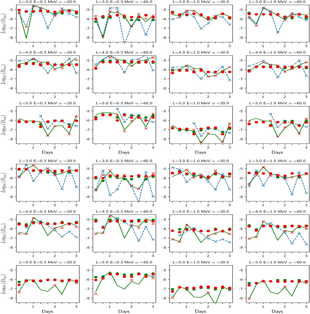
FIGURE 8. History of the storms 8 and 5. We plot here the same results as in Figure 5 (blue: raw data, red crosses (Kp, t, L, E, α) average model, green crosses (Kp, t, L, E, α) DNN model) to which we added circles obtained from averaging in time either the average data (red) or directly the DNN model (green); it produces a Kp-dependent (only) model. The DNN model approaches well its target (the average data) but both have a degraded accuracy compared to the event-driven model (in blue), particularly visible for storm 5 in which diffusion coefficients depart significantly from the average.
4.3 Model Limitations and Future Improvements
The data we use were not created specifically for this study and, as such, the discretization is not best optimized for further encapsulation by a machine learning method. The original set is too large for the herein regression in dimension 3 or 5 and the first task is a necessary strategy to reduce the amount of data. Moreover, when generating data for the purpose of machine learning modeling, an adaptive sampling strategy should be preferred. Such a method consists in optimizing at which variable in (L, E, α) the diffusion coefficient should be computed. This task is left for a future improvement of the model.
The present DNN model of HSS storms has been computed for 5 L-shells with a ΔL = 1. One of the next tasks is to generalize the method to 50 L-shells covering the whole domain with ΔL = 0.1. One way is to repeat the study but spread the teaching onto randomly chosen L-shells in order to keep the same resolution or to increase the sampling size, which remains possible with DNN.
Landau diffusion is the highest diffusion we see for pitch angle above αL > ∼ 80° in Figure 6 (top, left). At lower pitch angle, Landau diffusion is well defined but negligible (cf Mourenas and Ripoll [45] for an approximation of αL for a given L-shell and energy). For very large pitch angle, Landau diffusion is strong almost everywhere in the (L, E) plane, but this strong diffusion is surrounded by very weak diffusion outside [αL, 90 − ϵ], which traps and diffuses the particle within that pitch angle range. Only coupled energy-pitch angle diffusion effects can then change the electron pitch angle outside of that range [83]. The region of Landau diffusion is a region with a distinct behavior that requires particular attention and can cause the DNN network to make higher local errors (as discussed previously). There can be various strategies to avoid that difficulty. One can either choose to generate two distinct DNN models, one for low and moderate pitch angles (which has the effect to focus on cyclotron resonance) and the other for larger ones (above αL > ∼ 80° where Landau generally occurs). This strategy can be tricky because the exact position of the Landau resonance varies also with the wave and density properties [45] leading to a dependence with (t, Kp, L, E). The better and simpler strategy, which our study brings, is to separate the sum of the n-cyclotron harmonics of the diffusion coefficient from the Landau harmonic (n = 0) when the diffusion coefficients are computed and to store both. Then, it is straightforward and more accurate to build a DNN model for each of the two components: one for the n-cyclotron and one for the Landau component. The full model is then made by the sum of both models. The only drawback is the increase of the memory storage by a factor 2.
Finally, machine learning models provide a wide and continuous model in a high dimensional space, which can produce extrapolation and surprising results (right or wrong) in particular for rare events and in the various high-dimensional corners of the model. These solutions always require for verification to go back to the database and to explore it more and more to the point of knowing (or trying to know) the data in all its aspects. This is often very time consuming, if not practically impossible, even if facilitated by the machine learning method in use. These difficulties call for reliable and robust testing methods and metrics to be able to rely more and more on the machine learning method with less and less verification of the database. In this work, even though the DNN model has shown a good accuracy, we do not think we have yet reached this level as, for instance, there are some remaining issues due to strong gradients (e.g., associated to Landau diffusion) or there is no possibility to verify and validate the behavior of the model for special configuration (e.g., low Kp in the first time of the HSS storm). The second point may call for using a given mean model simultaneously with its variance, which signifies using DNN that propagate the distribution of the data. A mean answer would be given with a confidence index based on the variance. The generation of DNN-based median, quartile, and standard deviation of the diffusion coefficients is thus a promising next step to help selecting a given model. A second important application brought by the knowledge of both the mean and variance is the ability to perform with them uncertainty analysis of Fokker Planck simulation (e.g., [40]) and better establish the variability caused by storms and better rank the best possible scenarios for given conditions.
5 Conclusion
In this work, we consider 8 nonparametric methods of machine learning based on local evaluation (k-nearest neighbors and kernel regression), tree-based methods (regression tree, bagging and random forest), neural networks, and function approximations (Radial basis and splines). With them, we derive machine learning based models of event-driven diffusion coefficients first for the storm of March 2013 associated to high-speed streams. We present an approach that exhibits some selected properties of the machine learning models in order to select the best method for our problem among the 8 methods. The approach is based on 3 diagnostics: compute the main global metrics (including mean, median, minimum, maximum, standard deviation, and quartiles errors) at various resolution of the database, generate violin plots for analyzing the error distribution, and compute the correlation of each method with the other to enlighten their differences and exhibit the main families. We find that neural networks (DNN), radial basis functions, and splines methods performed the best for this storm, with DNN retained for the next steps of the study.
We then use the diffusion coefficients computed from 32 high-speed storms in order to build a statistical event-driven diffusion coefficient that is embedded within the retained DNN model. This is the first model of that kind for two reasons. First the machine learning model encapsulates the statistical event-driven diffusion coefficients. Second, this is the first statistical diffusion coefficients made from averaging event-driven coefficients. The common approach is to rather build statistical wave and plasma properties and to compute single diffusion coefficients from them.
The statistics of the event-driven diffusion coefficients are based on the mean with a double parametrization in epoch time and Kp. The double parametrization is chosen to keep both the strength of the storm and follow its history through epoch time. In comparison, a Kp-only model is found too inaccurate compared with specific event-driven diffusion coefficients (by 1–2 orders of magnitudes depending on the event). The machine learning model step is made for greatly facilitating the use of the mean model, for instance, in providing a continuous solution in a high dimensional space [e.g., (t, L, E, α, Kp)]. We find the DNN model does not entail any issue to interpolate the averaged model and reproduces quite perfectly its target. Some small deviations are found at very high pitch angle for Landau resonance for which we propose a future solution to bypass this difficulty. We then use the DNN mean model to analyze how mean diffusion coefficients behave compared with individual ones. We find a poor performance of any mean models compared with individual events, with mean models computing the general trend at best. Degradation of the accuracy of mean diffusion coefficients comes for the large variance of event-driven diffusion coefficients. Mean models can easily deviate by 2 orders of magnitude. This is shown to occur, for instance, in region of strong gradients of the diffusion coefficients, basically delimited by the edge of the first cyclotron resonance in the (E, α) plane.
The strength of the DNN approach is the simplicity of performing comparisons since the model delivers a continuous map of the solution with a simple numerical subroutine for a problem with 5–6 dimensions here. This is illustrated by model exploration provided in Section 3.2.3. Plotting diffusion coefficients in the (t, Kp) plane, for instance, shows a wide variety of solutions, contributing to explain why storms can be so different from one event to the other.
Machine learning methods and the easily accessible numerical procedures that favor their use have a wide potential for the type of problems we presented, whether it is for manipulating, interpolating, representing, or for analyzing a huge database of event-driven diffusion coefficients and, more generally, database of diffusion coefficients combined with the main parameters used to compute them, such as plasma density and wave parameters. An inherent drawback is the human involvement required to analyze these huge databases in order to potentially identify regions of model deviance or model breakthrough.
The DNN method that is proposed here has the advantage to be extended to more parameters characterizing storms (including OMNI solar wind and geomagnetic index data), which should improve the accuracy and predictability of global models. DNN can similarly be used to derive DNN-based median, quartile, and standard deviation of the diffusion coefficients. With them, one can perform uncertainty analysis of Fokker Planck simulation and better establish the variability caused by storms and better rank the best possible scenarios for given conditions. We expect this approach to take more importance in the coming years.
Data Availability Statement
Publicly available datasets were used in this study. EMFISIS data was obtained from https://emfisis. physics.uiowa.edu/Flight/. Data are also available at NASA CDAWeb https://cdaweb. gsfc.nasa.gov/index.html/. Datafiles and both RBF and KerReg models are hosted on https://github.com/ ML-Space-Weather/PADiffusion-HSS. For DNN models, we used DJINN package https: //github.com/LLNL/DJINN. It is based on scikit-learn and tensorflow library. The tree- based and local evaluation methods are based on sklearn library. We use both the tree and the neighbors functions for Regression tree and KNN, respectively. We use both BaggingRegressor and RandomForestRegressor functions of ensemble module (sklearn.ensemble) of sklearn, respectively. And we use KFold function of model selection module from sklearn to perform K-fold cross validation in selecting the hyperparameters of the methods. Lastly, the Thin Plate Spline regression was implemented in R software using Tps function of fields library https://cran. r-project.org/package=fields.
Author Contributions
All authors contributed to the manuscript and the data analysis, with a synthesis made by GK. Data were constructed by J-FR and processed by GK. J-FR, and EC brought their expertise in geophysics. SH, AF, MM, EC, and GK in machine learning. Models were made by SH, AF, MM, except for the radial basis model (EC) and the deep neural network learning model (GK). GK, and J-FR together wrote the first draft of the manuscript. J-FR performed the physical analysis. All authors contributed to manuscript revision, read, and approved the submitted version.
Funding
EC is partially funded by the National Aeronautics and Space Administration under grant 80NSSC20K1580 “SWQU: Ensemble Learning for Accurate and Reliable Uncertainty Quantification.”
Conflict of Interest
The authors declare that the research was conducted in the absence of any commercial or financial relationships that could be construed as a potential conflict of interest.
Publisher’s Note
All claims expressed in this article are solely those of the authors and do not necessarily represent those of their affiliated organizations, or those of the publisher, the editors, and the reviewers. Any product that may be evaluated in this article, or claim that may be made by its manufacturer, is not guaranteed or endorsed by the publisher.
References
1. Lyons LR, Thorne RM. Equilibrium Structure of Radiation belt Electrons. J Geophys Res (1973) 78:2142–9. doi:10.1029/JA078i013p02142
2. Mauk BH, Fox NJ, Kanekal SG, Kessel RL, Sibeck DG, Ukhorskiy A. Science Objectives and Rationale for the Radiation belt Storm Probes mission. Space Sci Rev (2013) 179:3–27. doi:10.1007/s11214-012-9908-y
3. Reeves GD, Friedel RHW, Larsen BA, Skoug RM, Funsten HO, Claudepierre SG, et al. Energy‐dependent Dynamics of keV to MeV Electrons in the Inner Zone, Outer Zone, and Slot Regions. J Geophys Res Space Phys (2016) 121:397–412. doi:10.1002/2015JA021569
4. Breneman AW, Halford A, Millan R, McCarthy M, Fennell J, Sample J, et al. Global-scale Coherence Modulation of Radiation-belt Electron Loss from Plasmaspheric Hiss. Nature (2015) 523:193–5. doi:10.1038/nature14515
5. Millan RM, McCarthy MP, Sample JG, Smith DM, Thompson LD, McGaw DG, et al. The Balloon Array for Rbsp Relativistic Electron Losses (Barrel). Space Sci Rev (2013) 179:503–30. doi:10.1007/s11214-013-9971-z
6. Millan RM, Ripoll J-F, Santolík O, Kurth WS. Early-time Non-equilibrium Pitch Angle Diffusion of Electrons by Whistler-Mode Hiss in a Plasmaspheric Plume Associated with Barrel Precipitation. Front Astron Space Sci (2021) 8. doi:10.3389/fspas.2021.776992
7. Ripoll J-F, Claudepierre SG, Ukhorskiy AY, Colpitts C, Li X, Fennell JF, et al. Particle Dynamics in the Earth’s Radiation Belts: Review of Current Research and Open Questions. J Geophys Res Space Phys (2020) 125:e2019JA026735. doi:10.1029/2019JA026735
8. Meredith NP, Horne RB, Glauert SA, Baker DN, Kanekal SG, Albert JM. Relativistic Electron Loss Timescales in the Slot Region. J Geophys Res Space Phys (2009) 114. doi:10.1029/2008ja013889
9. Li W, Ma Q, Thorne RM, Bortnik J, Kletzing CA, Kurth WS, et al. Statistical Properties of Plasmaspheric Hiss Derived from Van allen Probes Data and Their Effects on Radiation belt Electron Dynamics. J Geophys Res Space Phys (2015) 120:3393–405. doi:10.1002/2015JA021048
10. Meredith NP, Horne RB, Kersten T, Li W, Bortnik J, Sicard A, et al. Global Model of Plasmaspheric Hiss from Multiple Satellite Observations. J Geophys Res Space Phys (2018) 123:4526–41. doi:10.1029/2018JA025226
11. Ripoll J-F, Reeves GD, Cunningham GS, Loridan V, Denton M, Santolík O, et al. Reproducing the Observed Energy-dependent Structure of Earth's Electron Radiation Belts during Storm Recovery with an Event-specific Diffusion Model. Geophys Res Lett (2016) 43:5616–25. doi:10.1002/2016GL068869
12. Ripoll JF, Santolík GD, Kurth WS, Denton MH, Loridan V, et al. Effects of Whistler Mode Hiss Waves in March 2013. J Geophys Res Space Phys (2017) 122:7433–62. doi:10.1002/2017JA024139
13. Thorne RM, Li W, Ni B, Ma Q, Bortnik J, Chen L, et al. Rapid Local Acceleration of Relativistic Radiation-belt Electrons by Magnetospheric Chorus. Nature (2013) 504:411–4. doi:10.1038/nature12889
14. Réveillé T. Etude de mécanismes de pertes de particules dans les ceintures artificielles de van allen. FranceNancy-I: Univ. Henri Poincaré (1997). Ph.D. Thesis.
15. Watt CEJ, Allison HJ, Thompson RL, Bentley SN, Meredith NP, Glauert SA, et al. The Implications of Temporal Variability in Wave‐Particle Interactions in Earth's Radiation Belts. Geophys Res Lett (2021) 48:e2020GL089962. doi:10.1029/2020GL089962
16. Ripoll JF, Loridan V, Denton MH, Cunningham G, Reeves G, Santolík O, et al. Observations and Fokker‐Planck Simulations of the L ‐Shell, Energy, and Pitch Angle Structure of Earth's Electron Radiation Belts during Quiet Times. J Geophys Res Space Phys (2019) 124:1125–42. doi:10.1029/2018JA026111
17. Ripoll J-F, Denton MH, Hartley DP, Reeves GD, Malaspina D, Cunningham GS, et al. Scattering by Whistler-Mode Waves during a Quiet Period Perturbed by Substorm Activity. J Atmos Solar-Terrestrial Phys (2021) 215:105471. doi:10.1016/j.jastp.2020.105471
18. Sicard-Piet A, Boscher D, Horne RB, Meredith NP, Maget V. Effect of Plasma Density on Diffusion Rates Due to Wave Particle Interactions with Chorus and Plasmaspheric Hiss: Extreme Event Analysis. Ann Geophys (2014) 32:1059–71. doi:10.5194/angeo-32-1059-2014
19. Horne RB, Kersten T, Glauert SA, Meredith NP, Boscher D, Sicard‐Piet A, et al. A New Diffusion Matrix for Whistler Mode Chorus Waves. J Geophys Res Space Phys (2013) 118:6302–18. doi:10.1002/jgra.50594
20. Linty N, Farasin A, Favenza A, Dovis F. Detection of Gnss Ionospheric Scintillations Based on Machine Learning Decision Tree. IEEE Trans Aerospace Electron Syst (2018) 55:303–17.
21. McGranaghan RM, Mannucci AJ, Wilson B, Mattmann CA, Chadwick R. New Capabilities for Prediction of High-Latitude Ionospheric Scintillation: A Novel Approach with Machine Learning. Space Weather (2018) 16:1817–46. doi:10.1029/2018sw002018
22. Tulunay E, Senalp ET, Radicella SM, Tulunay Y. Forecasting Total Electron Content Maps by Neural Network Technique. Radio Sci (2006) 41. doi:10.1029/2005rs003285
23. Sun W, Xu L, Huang X, Zhang W, Yuan T, Chen Z, et al. Forecasting of Ionospheric Vertical Total Electron Content (Tec) Using Lstm Networks. 2017 International Conference on Machine Learning and Cybernetics (ICMLC). IEEE (2017). 2. 340–4. doi:10.1109/icmlc.2017.8108945
24. Cesaroni C, Spogli L, Aragon-Angel A, Fiocca M, Dear V, De Franceschi G, et al. Neural Network Based Model for Global Total Electron Content Forecasting. J Space Weather Space Clim (2020). doi:10.1051/swsc/2020013
25. Oyeyemi E, Poole A, McKinnell L. On the Global Model for Fof2 Using Neural Networks. Radio Sci (2005) 40. doi:10.1029/2004rs003223
26. Pérez D, Wohlberg B, Lovell TA, Shoemaker M, Bevilacqua R. Orbit-centered Atmospheric Density Prediction Using Artificial Neural Networks. Acta Astronautica (2014) 98:9–23.
27. McGranaghan RM, Ziegler J, Bloch T, Hatch S, Camporeale E, Lynch K, et al. Toward a Next Generation Particle Precipitation Model: Mesoscale Prediction through Machine Learning (A Case Study and Framework for Progress). Space Weather (2021), 19. p. e2020SW002684.
28. Gruet MA, Chandorkar M, Sicard A, Camporeale E. Multiple-hour-ahead Forecast of the Dst index Using a Combination of Long Short-Term Memory Neural Network and Gaussian Process. Space Weather (2018) 16:1882–96. doi:10.1029/2018sw001898
29. Siciliano F, Consolini G, Tozzi R, Gentili M, Giannattasio F, De Michelis P. Forecasting Sym-H index: A Comparison between Long Short-Term Memory and Convolutional Neural Networks. Space Weather (2021) 19:e2020SW002589. doi:10.1029/2020sw002589
30. Takalo J, Timonen J. Neural Network Prediction of Ae Data. Geophys Res Lett (1997) 24:2403–6. doi:10.1029/97gl02457
31. Bala R, Reiff P. Improvements in Short-Term Forecasting of Geomagnetic Activity. Space Weather (2012) 10. doi:10.1029/2012sw000779
32. Liemohn MW, McCollough JP, Jordanova VK, Ngwira CM, Morley SK, Cid C, et al. Model Evaluation Guidelines for Geomagnetic index Predictions. Space Weather (2018) 16:2079–102. doi:10.1029/2018sw002067
33. Zhelavskaya IS, Spasojevic M, Shprits YY, Kurth WS. Automated Determination of Electron Density from Electric Field Measurements on the Van allen Probes Spacecraft. J Geophys Res Space Phys (2016) 121:4611–25. doi:10.1002/2015JA022132
34. Zhelavskaya IS, Shprits YY, Spasojević M. Empirical Modeling of the Plasmasphere Dynamics Using Neural Networks. J Geophys Res Space Phys (2017) 122:11227–11244. doi:10.1002/2017JA024406
35. Zhelavskaya IS, Shprits YY, Spasojevic M. Reconstruction of Plasma Electron Density from Satellite Measurements via Artificial Neural Networks. In: E Camporeale, S Wing, and JR Johnson, editors. Machine Learning Techniques for Space Weather. Elsevier (2018). p. 301–27. doi:10.1016/B978-0-12-811788-0.00012-3
36. Chu XN, Bortnik J, Li W, Ma Q, Angelopoulos V, Thorne RM. Erosion and Refilling of the Plasmasphere during a Geomagnetic Storm Modeled by a Neural Network. J Geophys Res Space Phys (2017) 122:7118–29. doi:10.1002/2017JA023948
37. Chu X, Bortnik J, Li W, Ma Q, Denton R, Yue C, et al. A Neural Network Model of Three‐dimensional Dynamic Electron Density in the Inner Magnetosphere. J Geophys Res Space Phys (2017) 122:9183–97. doi:10.1002/2017JA024464
38. Ma Q, Li W, Bortnik J, Thorne RM, Chu X, Ozeke LG, et al. Quantitative Evaluation of Radial Diffusion and Local Acceleration Processes during Gem challenge Events. J Geophys Res Space Phys (2018) 123:1938–52. doi:10.1002/2017JA025114
39. Malaspina DM, Ripoll JF, Chu X, Hospodarsky G, Wygant J. Variation in Plasmaspheric Hiss Wave Power with Plasma Density. Geophys Res Lett (2018) 45:9417–26. doi:10.1029/2018GL078564
40. Camporeale E, Chu X, Agapitov OV, Bortnik J. On the Generation of Probabilistic Forecasts from Deterministic Models. Space Weather (2019) 17:455–75. doi:10.1029/2018sw002026
41. Wang D, Shprits YY, Zhelavskaya IS, Effenberger F, Castillo AM, Drozdov AY, et al. The Effect of Plasma Boundaries on the Dynamic Evolution of Relativistic Radiation belt Electrons. J Geophys Res Space Phys (2020) 125:e2019JA027422. doi:10.1029/2019JA027422
42. Camporeale E. The challenge of Machine Learning in Space Weather: Nowcasting and Forecasting. Space Weather (2019) 17:1166–207. doi:10.1029/2018SW002061
43. Turner DL, Kilpua EKJ, Hietala H, Claudepierre SG, O’Brien TP, Fennel JF, et al. The Response of Earth's Electron Radiation Belts to Geomagnetic Storms: Statistics from the Van Allen Probes Era Including Effects from Different Storm Drivers. J Geophys Res Space Phys (2019) 124:1013–34. doi:10.1029/2018JA026066
44. Lyons LR, Thorne RM, Kennel CF. Pitch-angle Diffusion of Radiation belt Electrons within the Plasmasphere. J Geophys Res (1972) 77:3455–74. doi:10.1029/JA077i019p03455
45. Mourenas D, Ripoll J-F. Analytical Estimates of Quasi-Linear Diffusion Coefficients and Electron Lifetimes in the Inner Radiation belt. J Geophys Res (2012) 117. doi:10.1029/2011JA016985
46. Albert JM. Evaluation of Quasi-Linear Diffusion Coefficients for Whistler Mode Waves in a Plasma with Arbitrary Density Ratio. J Geophys Res (2005) 110. doi:10.1029/2004JA010844
47. Réveillé T, Bertrand P, Ghizzo A, Simonet F, Baussart N. Dynamic Evolution of Relativistic Electrons in the Radiation Belts. J Geophys Res Space Phys (2001) 106:18883–94. 10.1029/2000JA900177.
48. Albert JM. Analysis of Quasi-Linear Diffusion Coefficients. J Geophys Res (1999) 104:2429–41. doi:10.1029/1998JA900113
49. Albert JM. Quasi-linear Pitch Angle Diffusion Coefficients: Retaining High Harmonics. J Geophys Res (1994) 99:23741–5. doi:10.1029/94JA02345
50. Albert JM. Efficient Approximations of Quasi-Linear Diffusion Coefficients in the Radiation Belts. J Geophys Res (2008) 113:a–n. doi:10.1029/2007JA012936
51. Meredith NP, Horne RB, Glauert SA, Anderson RR. Slot Region Electron Loss Timescales Due to Plasmaspheric Hiss and Lightning-Generated Whistlers. J Geophys Res (2007) 112:a–n. doi:10.1029/2007JA012413
52. Ripoll J-F, Mourenas D. High-Energy Electron Diffusion by Resonant Interactions with Whistler Mode Hiss. American Geophysical Union AGU (2012). p. 281–90. doi:10.1029/2012GM001309
53. Loridan V, Ripoll JF, Tu W, Scott Cunningham G. On the Use of Different Magnetic Field Models for Simulating the Dynamics of the Outer Radiation belt Electrons during the October 1990 Storm. J Geophys Res Space Phys (2019) 124:6453–86. doi:10.1029/2018JA026392
54. Ripoll JF, Loridan V, Cunningham GS, Reeves GD, Shprits YY. On the Time Needed to Reach an Equilibrium Structure of the Radiation Belts. J Geophys Res Space Phys (2016) 121:7684–98. doi:10.1002/2015JA022207
55. Santolík O, Parrot M, Storey LRO, Pickett JS, Gurnett DA. Propagation Analysis of Plasmaspheric Hiss Using Polar Pwi Measurements. Geophys Res Lett (2001) 28:1127–30. doi:10.1029/2000GL012239
56. Kletzing CA, Kurth WS, Acuna M, MacDowall RJ, Torbert RB, Averkamp T, et al. The Electric and Magnetic Field Instrument Suite and Integrated Science (Emfisis) on Rbsp. Space Sci Rev (2013) 179:127–81. doi:10.1007/s11214-013-9993-6
57. Spasojevic M, Shprits YY, Orlova K. Global Empirical Models of Plasmaspheric Hiss Using Van allen Probes. J Geophys Res Space Phys (2015) 120:10370–10383. doi:10.1002/2015JA021803
58. Kurth WS, De Pascuale S, Faden JB, Kletzing CA, Hospodarsky GB, Thaller S, et al. Electron Densities Inferred from Plasma Wave Spectra Obtained by the Waves Instrument on Van allen Probes. J Geophys Res Space Phys (2015) 120:904–14. doi:10.1002/2014JA020857
59. Thaller SA, Wygant JR, Dai L, Breneman AW, Kersten K, Cattell CA, et al. Van Allen Probes Investigation of the Large‐scale Duskward Electric Field and its Role in Ring Current Formation and Plasmasphere Erosion in the 1 June 2013 Storm. J Geophys Res Space Phys (2015) 120:4531–43. doi:10.1002/2014JA020875
60. Wygant JR, Bonnell JW, Goetz K, Ergun RE, Mozer FS, Bale SD, et al. The Electric Field and Waves Instruments on the Radiation belt Storm Probes mission. Space Sci Rev (2013) 179:183–220. doi:10.1007/s11214-013-0013-7
61. Cervantes S, Shprits YY, Aseev NA, Allison HJ. Quantifying the Effects of Emic Wave Scattering and Magnetopause Shadowing in the Outer Electron Radiation belt by Means of Data Assimilation. J Geophys Res Space Phys (2020) 125:e2020JA028208. doi:10.1029/2020JA028208
62. Baker DN, Jaynes AN, Li X, Henderson MG, Kanekal SG, Reeves GD, et al. Gradual Diffusion and Punctuated Phase Space Density Enhancements of Highly Relativistic Electrons: Van allen Probes Observations. Geophys Res Lett (2014) 41:1351–8. doi:10.1002/2013GL058942
63. Li Z, Hudson M, Jaynes A, Boyd A, Malaspina D, Thaller S, et al. Modeling Gradual Diffusion Changes in Radiation belt Electron Phase Space Density for the March 2013 Van allen Probes Case Study. J Geophys Res Space Phys (2014) 119:8396–403. doi:10.1002/2014JA020359
67. Fix E, Hodges J. Discriminatory Analysis. Nonparametric Discrimination: Consistency Properties (Report). Tech. rep. (1951).
68. Altman NS. An Introduction to Kernel and Nearest-Neighbor Nonparametric Regression. The Am Statistician (1992) 46:175–85. doi:10.1080/00031305.1992.10475879
70. Watson GS. Smooth Regression Analysis. Sankhyā: Indian J Stat Ser A (1964) 26:359–72. doi:10.1136/hrt.26.6.755
71. Breiman L, Friedman JH, Olshen RA, Stone CJ. Classification and Regression. Trees, CA: Wadsworth and Brooks/Cole Advanced Books and Software (1984).
73. Ho TK. Random Decision Forests. Proceedings of the Third International Conference on Document Analysis and Recognition. 1. USA: IEEE Computer Society (1995). p. 278.
75. Cybenko G. Approximations by Superpositions of Sigmoidal Functions. Mathematics Control Signals ans Syst (1989) 2. doi:10.1007/bf02551274
76. Humbird KD, Peterson JL, McClarren RG. Deep Neural Network Initialization with Decision Trees. IEEE Trans Neural Netw Learn Syst (2019) 30:1286–95. doi:10.1109/TNNLS.2018.2869694
77. Kluth G, Humbird K, Spears B, Peterson J, Scott H, Patel M, et al. Deep Learning for Nlte Spectral Opacities. Phys plasma (2020) 27. doi:10.1063/5.0006784
78. Duchon J. Splines Minimizing Rotation-Invariant Semi-norms in Sobolev Spaces. In: Construction Theory of Functions of Several Variables. Berlin: Springer (1977). doi:10.1007/bfb0086566
79. Green PJ, Silverman BW. Nonparametric Regression and Generalized Linear Models: A Roughness Penalty Approach. United Kingdom: Chapman & Hall (1994).
80. Reeves GD, Baker DN, Belian RD, Blake JB, Cayton TE, Fennell JF, et al. The Global Response of Relativistic Radiation belt Electrons to the January 1997 Magnetic Cloud. Geophys Res Lett (1998) 25:3265–8. doi:10.1029/98GL02509
81. Zhu H, Shprits YY, Spasojevic M, Drozdov AY. New Hiss and Chorus Waves Diffusion Coefficient Parameterizations from the Van allen Probes and Their Effect on Long-Term Relativistic Electron Radiation-belt Verb Simulations. J Atmos Solar-Terrestrial Phys (2019) 193:105090. doi:10.1016/j.jastp.2019.105090
82. Ripoll J-F, Kluth G, Has S, Fischer A, Mougeot M, Camporeale E. A Neural Network Model of Quasi-Linear Diffusion Coefficients during High-Speed Streams. Proceedings of the 3rd URSI AT-AP-RASC, Gran Canaria, 29 May – 3 June 2022 (2022).
Keywords: machine learning, pitch angle diffusion, event-driven, data exploration, high speed streams
Citation: Kluth G, Ripoll J-F, Has S, Fischer A, Mougeot M and Camporeale E (2022) Machine Learning Methods Applied to the Global Modeling of Event-Driven Pitch Angle Diffusion Coefficients During High Speed Streams. Front. Phys. 10:786639. doi: 10.3389/fphy.2022.786639
Received: 30 September 2021; Accepted: 21 February 2022;
Published: 05 May 2022.
Edited by:
Georgios Balasis, National Observatory of Athens, GreeceReviewed by:
Jorge Amaya, KU Leuven, BelgiumDedong Wang, GFZ German Research Centre for Geosciences, Germany
Antoine Brunet, Université de Toulouse, France
Copyright © 2022 Kluth , Ripoll , Has , Fischer , Mougeot and Camporeale . This is an open-access article distributed under the terms of the Creative Commons Attribution License (CC BY). The use, distribution or reproduction in other forums is permitted, provided the original author(s) and the copyright owner(s) are credited and that the original publication in this journal is cited, in accordance with accepted academic practice. No use, distribution or reproduction is permitted which does not comply with these terms.
*Correspondence: G. Kluth , gilles.kluth@cea.fr