Inverse Solution of Thermoacoustic Wave Equation for Cylindrical Layered Media

Thermoacoustic imaging is a crossbred approach taking advantages of electromagnetic and ultrasound disciplines, together. A significant number of current medical imaging strategies are based on reconstruction of source distribution from information collected by sensors over a surface covering the region to be imaged. Reconstruction in thermoacoustic imaging depends on the inverse solution of thermoacoustic wave equation. Homogeneous assumption of tissue to be imaged results in degradation of image quality. In our paper, inverse solution of the thermoacoustic wave equation using layered tissue model consisting of concentric annular layers on a cylindrical cross-section is investigated for cross-sectional thermoacustic imaging of breast and brain. By using Green’s functions and surface integral methods we derive an exact analytic inverse solution of thermoacoustic wave equation in frequency domain. Our inverse solution is an extension of conventional solution to layered cylindrical structures. By carrying out simulations, using numerical test phantoms consisting of thermoacoustic sources distributed in the layered model, our layered medium assumption solution was tested and benchmarked with conventional solutions based on homogeneous medium assumption in frequency domain. In thermoacoustic image reconstruction, where the medium is assumed as homogeneous medium, the solution of nonhomogeneous thermoacoustic wave equation results in geometrical distortions, artifacts and reduced image resolution due to inconvenient medium assumptions.

1 Introduction

In thermoacoustic imaging, non-ionizing radio frequency or microwave pulses are delivered in to biological tissues. Some of the delivered energy is absorbed and converted into heat, leading to thermoelastic expansion, which in turn leads to ultrasonic emission. The generated ultrasonic waves are then detected by ultrasonic transducers located on the boundary of the object in order to form images of absorption properties of the object. Reconstruction of source distribution (absorption function) is based on the inverse solution of thermoacoustic wave equation. Most of the research studies reported in the literature were based on inverse solution of thermoacoustic wave equation using homogeneous medium assumption [1], [2]. The boundary conditions for thermoacoustic imaging have been investigated by Wang and Yang [3]. In a more recent study, Schoonover and Anastasio have presented an inverse solution based on piecewise homogeneous planar layers structure consisting source distribution only in one certain layer [4]. Also, there are other studies taking acoustic heterogeneties into account combining conventional methods and acoustic speed distribution as apriori information so that reducing effect of inhomogeneity and improving image quality [5–8]. Here our approach is based on the facts that two-dimensional cross-sections of many organs and tissue structures such as breast and brain can efficiently be modelled by piecewise homogeneous cylindrical layers and thermoacoustic sources are distributed over all layer structure. Thus, in this study, for cross-sectional two-dimensional thermoacustic imaging of breast and brain, we explore solution of the wave equation using layered tissue model consisting of concentric annular layers on a cylindrical cross-section. At first, we state the inverse source problem concerning thermoacoustic wave equation on a nonhomogeneous medium and describe the layered cylindrical medium; and then we derive the Green’s function of described media involving Bessel and Hankel functions to obtain the forward and inverse solutions of the nonhomogeneous thermoacoustic wave equation. The geometrical and acoustic parameters (densities and velocities) of layered media are utilized together with temporal initial condition, radiation conditions and continuity conditions on the layers’ boundaries. After, we give a forward solution and represent a key property of Green’s function resulting from initial condition of thermoacoustic wave propagation, and using this, we derive an exact analytic inverse solution of thermoacoustic wave equation for N-layered media. Lastly, to test and compare our layered solution with conventional solution based on homogeneous medium assumption, we performed simulations using numerical test phantoms consisting of sources distributed in the layered structure. The image reconstruction based on this approach involves the layer parameters as the apriori information which can be estimated from the acquired thermoacoustic data or additional transmission ultrasound scan.

2 Problem Statement

Consider a region having (N − 1) concentric annular cylindrical layers with different acoustic properties in the space ${\mathbb{R}}^3$ where its z-cross-section as depicted in the Figure 1. The interface of consecutive mth and (m + 1)^th layers is a cylinder with center (0, 0) and radius r = r_m, denoted by S_m (m = 1, … , N − 1). Suppose there is a cylindrical transducer in outside of layered cylindrical structure called S_N closing the other regions as in the Figure 1. We call the volume covered by transducer S_N as V. We want to determine the source distribution of the region covered by transducer.

FIGURE 1

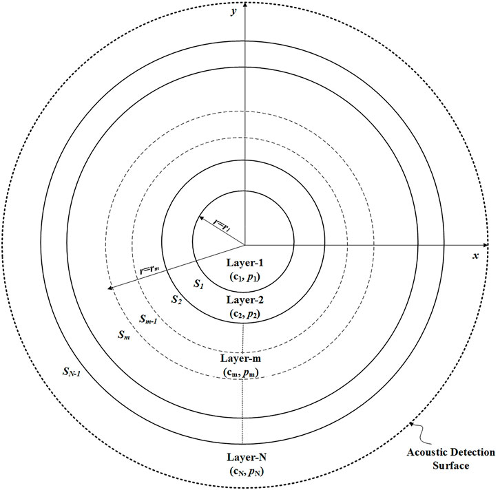
FIGURE 1. Z-Cross section of N-Layered medium.

The acoustic waves are measured by the transducer for a sufficiently long time interval so that the waves emitted from every source location reach to the transducer. When the regions are different, there will be reflections and transmissions at the boundaries, S_m, for 1 ≤ m ≤ N − 1. Hence, the thermoacoustic wave propagation is governed by the non-homogeneous wave equation for the pressure

${\nabla }^{2}p\left(\mathbf{r},t\right)-\frac{1}{c^2}\frac{{\partial }^{2}p}{{\partial t}^2}=-\frac{p_0\left(\mathbf{r}\right)}{c^2}.{\delta }^{\prime }\left(t\right)(1)$

with 2(N − 1) boundary conditions

$p_m\left(\mathbf{r},t\right)=p_{m+1}{\left.\left(\mathbf{r},t\right)\right|}_{\mathbf{r}\in S_m}(2)$

and

$\frac{1}{{\rho }_m}\frac{\partial p_m\left(\mathbf{r},t\right)}{\partial n}=\frac{1}{{\rho }_{m+1}}{\left.\frac{\partial p_{m+1}\left(\mathbf{r},t\right)}{\partial n}\right|}_{\mathbf{r}\in S_m}(3)$

on each boundary S_m. Here, p_m and p_m+1 are the pressure representing acoustic waves, ρ_m and ρ_m+1 are the densities for Region m and Region m + 1, respectively, and − p₀(r).δ′(t) is the source term emitting the thermoacoustic wave [9–13]. Also, the pressure function assures radiation condition. As the nature of the problem, thermoacoustic pressure function must satisfy the following initial conditions

$p\left(\mathbf{r},0^{+}\right)=p_0\left(\mathbf{r}\right)\text{and}\frac{\partial p\left(\mathbf{r},0^{+}\right)}{\partial t}=0(4)$

$p\left(\mathbf{r},t\right)=0\text{if}t<0.(5)$

In an inverse source problem, p₀(r) is to be reconstructed given that acoustic field is measured by the transducer and is known on the surface S_N.

To solve inverse problem, we firstly derive Green’s functions and state the forward solution of the problem by using Green’s function method. The Equation 1 in frequency domain corresponds to the nonhomogeneous three dimensional Helmholtz equation

${\nabla }^{2}P\left(\mathbf{r},w\right)+k^{2}P\left(\mathbf{r},w\right)=-iw\frac{p_0\left(\mathbf{r}\right)}{c^2},(6)$

where P(r, w) is the temporal Fourier Transform of p(r, t) and ${\nabla }^2={\nabla }_x^2+{\nabla }_y^2+{\nabla }_z^2$. Through the following derivations, we consider that w > 0 and than, by definition of Fourier transform, we write P(r, − w) = P(r,w)^∗ for w < 0 as complex conjugate of pressure function for positive frequency for the completeness in frequency domain.

The outgoing and incoming waves are represented by superscripts ‘out’ and ‘in’ for pressure function and we use the fact that $P^{in}(\mathbf{r},w)={\left(P^{out}(\mathbf{r},w)\right)}^{\ast }$.

3 Green’s Function of Medium

The Green’s function is the solution of homogeneous wave equation except the point r′ where the point source located:

${\nabla }^2{G}^{out}\left({\mathbf{r}}^{\prime },\mathbf{r},w\right)+k^2{G}^{out}\left({\mathbf{r}}^{\prime },\mathbf{r},w\right)=-\delta \left(\mathbf{r}-{\mathbf{r}}^{\prime }\right)(7)$

where δ(.) is the Dirac delta function.

It is convenient to study in cylindrical coordinates for the N-layered cylindrical configuration. Before transforming the Helmholtz equation Eq. 7 to cylindrical system, we take the spatial Fourier transform in z-direction to derive forward solution. We represent the spatial transform with a tilde symbol above of a function name, that is

$\tilde{f}\left(k_z\right)=\underset{-\infty }{\overset{\infty }{\int }}f\left(z\right)e^{-i{k}_{z}z}dz,(8)$

and from Eq. 7, we obtain two dimensional Helmholtz equation

${\nabla }^2\tilde{G}\left({\mathbf{r}}^{\prime },\mathbf{r},k_z,w\right)+\left(k^2-k_z^2\right)\tilde{G}\left({\mathbf{r}}^{\prime },\mathbf{r},k_z,w\right)=\delta \left(\mathbf{r}-{\mathbf{r}}^{\prime }\right)e^{-i{k}_z{z}^{\prime }}(9)$

where k = w/c is the wave number, k_z is the spatial frequency. The wave equation given in Eq. 9 is expressed in cylindrical coordinates (r, ϕ, z) as

$\frac{{\partial }^2\tilde{G}}{{\partial r}^2}+\frac{1}{r}\frac{\partial \tilde{G}}{\partial r}+\frac{1}{r^2}\frac{{\partial }^2\tilde{G}}{{\partial \varphi }^2}+\left(k^2-k_z^2\right)\tilde{G}=\frac{1}{r}\delta \left(r-r^{\prime }\right)\delta \left(\varphi -{\varphi }^{\prime }\right)e^{-i{k}_z{z}^{\prime }}.(10)$

It is known that the solution of above equation has a series form consisting of Bessel’s functions and exponential functions [14]. When $\sqrt{(k^2-k_z^2)}$ is a real number, the solution includes first and second kind of Bessel functions $J_n(\sqrt{(k^2-k_z^2)}r)$, $Y_n(\sqrt{(k^2-k_z^2)}r)$, respectively. On the other hand, when $\sqrt{(k^2-k_z^2)}$ is not a real number (in this case it is purely imaginary), the two independent solutions are first and second kind modified Bessel functions, $I_n(\sqrt{(k_z^2-k^2)}r)$ and $K_n(\sqrt{(k_z^2-k^2)}r)$, respectively. In this aspect, if we call terms $\sqrt{(k^2-k_z^2)}=\bar{k}$ and $\sqrt{(k_z^2-k^2)}r=\bar{q}$, the solution of Eq. 7 can be written as

$G\left({\mathbf{r}}^{\prime },\mathbf{r},w\right)=\left\{\begin{array}{c}\underset{-\infty }{\overset{\infty }{\int }}{e}^{i{k}_z\left(z-z^{\prime }\right)}\sum _{n=-\infty }^{\infty }\left({\alpha }_n{J}_n\left(\bar{k}r\right)+{\beta }_n{Y}_n\left(\bar{k}r\right)\right)e^{in\varphi }d{k}_z,\text{if\hspace{0.17em}}\parallel k\parallel \ge \parallel k_z\parallel \hfill \\ \underset{-\infty }{\overset{\infty }{\int }}{e}^{i{k}_z\left(z-z^{\prime }\right)}\sum _{n=-\infty }^{\infty }\left({\gamma }_n{I}_n\left(\bar{q}r\right)+{\zeta }_n{K}_n\left(\bar{q}r\right)\right)e^{in\varphi }d{k}_z,\text{if\hspace{0.17em}}\parallel k\parallel \le \parallel k_z\parallel \hfill \end{array}\right.(11)$

in which r = (r, ϕ, z) and r′ = (r′, ϕ′, z′).The Bessel functions J_n(.), Y_n(.), I_n(.) and K_n(.) are real valued functions for positive real arguments. Hence all the terms in summations except unknown coefficients in Eq. 11 are all real. When ∥ k ∥≥∥ k_z ∥ we apply Sommerfeld radiation condition and when ∥ k ∥ ≤ ∥ k_z ∥ we choose evanescent waves for outer most layer, so that the waves will not grow to infinity. In light of these, the derivations made for the argument $\bar{k}=\sqrt{(k^2-k_z^2)}r$ are the same as the derivations made for the argument $\bar{q}=\sqrt{(k_z^2-k^2)}r$ in inverse solution proof. Therefore, we only show the case ∥ k ∥≥∥ k_z ∥ in this paper.

When the point source r′ locates in Layer m, we denote Green’s function as G_m (1 ≤ m ≤ N). Each Green’s function G_m represents the unit impulse response of the layered medium and is partially defined with respect to observation point r:

$G_m\left({\mathbf{r}}^{\prime },\mathbf{r},w\right)=$

$\left\{\begin{array}{c}\sum _{n=-\infty }^{\infty }{e}^{in\varphi }{\int }_{-\infty }^{\infty }{e}^{i{k}_z\left(z-z^{\prime }\right)}\left(A_{nj}{J}_n\left({\bar{k}}_{j}r\right)+B_{nj}{Y}_n\left({\bar{k}}_{j}r\right)\right)d{k}_z,\text{if\hspace{0.17em}}r<r^{\prime }\text{and\hspace{0.17em}r\hspace{0.17em}in\hspace{0.17em}layer\hspace{0.17em}j}\hfill \\ \sum _{n=-\infty }^{\infty }{e}^{in\varphi }{\int }_{-\infty }^{\infty }{e}^{i{k}_z\left(z-z^{\prime }\right)}\left(C_{nj}{J}_n\left({\bar{k}}_{j}r\right)+D_{nj}{Y}_n\left({\bar{k}}_{j}r\right)\right)d{k}_z,\text{if\hspace{0.17em}}{r}^{\prime }<r\text{and\hspace{0.17em}r\hspace{0.17em}in\hspace{0.17em}layer\hspace{0.17em}j}\hfill \end{array}\right.(12)$

We call the parts of G_m as G_mj for 1 ≤ j ≤ N when observation point r in Layer j. In the derivations of inverse problem, the observation points are on the transducer in Layer N so we need to calculate only the last parts G_mN of Green’s function G_m wherever the source location m is

The coefficients in each Green’s function G_m are obtained by (2N + 2) equalities coming from the boundary conditions, Green’s functions conditions and radiation conditions: The given boundary conditions Eqs 2, 3 state that acoustic pressure function is continuous and its normal derivative is continuous with a scaling factor on the layer boundaries r = r_i:

$\begin{array}{ll}\hfill & A_{n\left(i+1\right)}{J}_n\left({\bar{k}}_{i+1}{r}_i\right)+B_{n\left(i+1\right)}{Y}_n\left({\bar{k}}_{i+1}{r}_i\right)-A_{n\left(i\right)}{J}_n\left({\bar{k}}_i{r}_i\right)-B_{n\left(i\right)}{Y}_n\left({\bar{k}}_i{r}_i\right)=0,\hfill \\ \hfill & \frac{{\bar{k}}_{i+1}}{{\rho }_{i+1}}\left(A_{n\left(i+1\right)}{J}_n^{\prime }\left({\bar{k}}_{i+1}{r}_i\right)+B_{n\left(i+1\right)}{Y}_n^{\prime }\left({\bar{k}}_{i+1}{r}_i\right)\right)-\frac{{\bar{k}}_i}{{\rho }_i}\left(A_{n\left(i\right)}{J}_n^{\prime }\left({\bar{k}}_i{r}_i\right)+B_{n\left(i\right)}{Y}_n^{\prime }\left({\bar{k}}_i{r}_i\right)\right)=0\hfill \end{array}(13)$

for 1 ≤ i ≤ m − 1,

$\begin{array}{ll}\hfill & C_{n\left(i+1\right)}{J}_n\left({\bar{k}}_{i+1}{r}_i\right)+D_{n\left(i+1\right)}{Y}_n\left({\bar{k}}_{i+1}{r}_i\right)-C_{n\left(i\right)}{J}_n\left({\bar{k}}_i{r}_i\right)-D_{n\left(i\right)}{Y}_n\left({\bar{k}}_i{r}_i\right)=0,\hfill \\ \hfill & \frac{{\bar{k}}_{i+1}}{{\rho }_{i+1}}\left(C_{n\left(i+1\right)}{J}_n^{\prime }\left({\bar{k}}_{i+1}{r}_i\right)+D_{n\left(i+1\right)}{Y}_n^{\prime }\left({\bar{k}}_{i+1}{r}_i\right)\right)-\frac{{\bar{k}}_i}{{\rho }_i}\left(C_{n\left(i\right)}{J}_n^{\prime }\left({\bar{k}}_i{r}_i\right)+D_{n\left(i\right)}{Y}_n^{\prime }\left({\bar{k}}_i{r}_i\right)\right)=0\hfill \end{array}(14)$

for m ≤ i ≤ N − 1.

On the other hand, Green’s function is continuous and its normal derivative has jump discontinuity on a cylinder r = r′ where the point source locates [16]. Hence, these conditions give us

$C_{n\left(m\right)}{J}_n\left({\bar{k}}_m{r}^{\prime }\right)+D_{n\left(m\right)}{Y}_n\left({\bar{k}}_m{r}^{\prime }\right)-A_{n\left(m\right)}{J}_n\left({\bar{k}}_m{r}^{\prime }\right)-B_{n\left(m\right)}{Y}_n\left({\bar{k}}_m{r}^{\prime }\right)=0,$

${\bar{k}}_m{r}^{\prime }\left(\left(C_{n\left(m\right)}-A_{n\left(m\right)}\right)J_n^{\prime }\left({\bar{k}}_m{r}^{\prime }\right)+\left(D_{n\left(m\right)}-B_{n\left(m\right)}\right)Y_n^{\prime }\left({\bar{k}}_m{r}^{\prime }\right)\right)=e^{-i{k}_z{z}^{\prime }}\frac{e^{-in{\varphi }^{\prime }}}{2\pi }.(15)$

Additionally, second kind of Bessel function Y_n is undefined when r = 0. Therefore in Layer 1, Green’s function cannot include Y_n implying

$B_{n1}=0.(16)$

Lastly, the pressure function must satisfy Sommerfeld radiation condition

${\lim }_{|\mathbf{r}|\to \infty }\left(\frac{\partial }{\partial |\mathbf{r}|}-ik\right)P\left(\mathbf{r},w\right)=0.(17)$

By writing Bessel functions J_n and Y_n in a linear combination of Hankel functions $H_n^1$ and $H_n^2$ in Layer N, we apply this acoustic attenuation condition property which eliminates $H_n^2$ and so we get

$D_{n\left(N\right)}+i{C}_{n\left(N\right)}=0.(18)$

We can write the system of equations in the matrix form as follows:

${\mathbf{B}}_{\mathbf{n}}.{\left[\begin{array}{cccccccc}\hfill A_{n1}\hfill & \hfill B_{n1}\hfill & \hfill \dots \hfill & \hfill B_{n\left(m\right)}\hfill & \hfill C_{n\left(m\right)}\hfill & \hfill C_{n\left(m+1\right)}\hfill & \hfill \dots \hfill & \hfill D_{n\left(N\right)}\hfill \end{array}\right]}^T={\left[\begin{array}{ccccccccc}\hfill 0\hfill & \hfill 0\hfill & \hfill \dots \hfill & \hfill 0\hfill & \hfill e^{-i{k}_z{z}^{\prime }}\frac{e^{-in{\varphi }^{\prime }}}{2\pi }\hfill & \hfill 0\hfill & \hfill \dots \hfill & \hfill 0\hfill & \hfill 0\hfill \\ \hfill \hfill \end{array}\right]}^T(19)$

in which M_n is the coefficient matrix (A.1) given in Supplementary Appendix. Here, when the point source location changes, the coefficient matrix of a system will differ. But, we show that for all possible matrix systems results from location of source point, the determinant of coefficient matrices are the same. (See Supplementary Appendix to find derivation of this fact). As a result, determinant of coefficient matrix M_n, say M_n, is independent of the source location and the same for all n (index set for Bessel functions’ order) and for all m (location of source point r′).

In the derivation of inverse solution, we need the last part of Green’s function G_m Eq. 12, that is G_mN. The coefficient D_n(N) in G_mN is obtained by Kramer’s rule as follows:

$D_{n\left(N\right)}=e^{-i{k}_z{z}^{\prime }}\frac{e^{-in{\varphi }^{\prime }}}{2\pi }\frac{R_n^m}{M_n}(20)$

in which $R_n^m$ is determinant expression (A.4) given in Supplementary Appendix. Here, the most important property of $R_n^m$ used in inverse problem derivation is that all the terms contained in $R_n^m$ are real, hence the determinant $R_n^m$ is itself is real. At the end, G_mN(r′, r, w) is written in the following form by using radiation condition result Eq. 18:

$\begin{array}{ll}\hfill & G_{mN}\left({\mathbf{r}}^{\prime },\mathbf{r},w\right)\hfill \\ \hfill & =\sum _{n=-\infty }^{\infty }{e}^{in\varphi }{\int }_{-\infty }^{\infty }{e}^{i{k}_{z}z}\left(-i{e}^{-i{k}_z{z}^{\prime }}\frac{e^{-in{\varphi }^{\prime }}}{2\pi }\frac{R_n^m}{M_n}\left(r^{\prime },r\right)J_n\left({\bar{k}}_{N}r\right)+e^{-i{k}_z{z}^{\prime }}\frac{e^{-in{\varphi }^{\prime }}}{2\pi }\frac{R_n^m}{M_n}\left(r^{\prime },r\right)Y_n\left({\bar{k}}_{N}r\right)\right)d{k}_z\hfill \\ \hfill & =\sum _{n=-\infty }^{\infty }\frac{e^{in\left(\varphi -{\varphi }^{\prime }\right)}}{2\pi }{\int }_{-\infty }^{\infty }{e}^{i{k}_z\left(z-z^{\prime }\right)}\frac{R_n^m}{M_n}\left(r^{\prime },r\right)\left(-i{H}_n^1\left({\bar{k}}_{N}r\right)\right)d{k}_z.\hfill \end{array}(21)$

4 Forward Solution and Initial Condition Yields

If the source distribution in the medium is p₀(r) and Green’s function of the medium is G(r, r′, w), then the forward solution of thermoacoustic wave equation in frequency domain can be written as [15], [16]

$P\left(\mathbf{r},w\right)=-iw{\int }_V\frac{p_0\left({\mathbf{r}}^{\prime }\right)}{c^2\left({\mathbf{r}}^{\prime }\right)}{G}^{out}\left(\mathbf{r},{\mathbf{r}}^{\prime },w\right)d{V}_{{\mathbf{r}}^{\prime }}(22)$

by make use of Green’s theorem and radiation conditions. Here, V is the support of source function. When we take the inverse Fourier transform of both sides of above forward solution at the discontinuity t = 0, we get

$\frac{1}{2}\left(p\left(\mathbf{r},0^{-}\right)+p\left(\mathbf{r},0^{+}\right)\right)=-\frac{i}{2\pi }{\int }_{-\infty }^{\infty }{\int }_{V}w\frac{p_0\left({\mathbf{r}}^{\prime }\right)}{c^2\left({\mathbf{r}}^{\prime }\right)}G\left(\mathbf{r},{\mathbf{r}}^{\prime },w\right)d{V}_{{\mathbf{r}}^{\prime }}dw.(23)$

By the initial condition of the thermoacoustic wave equation, we obtain

$p_0\left(\mathbf{r}\right)=-\frac{i}{\pi }{\int }_{-\infty }^{\infty }{\int }_{V}w\frac{p_0\left({\mathbf{r}}^{\prime }\right)}{c^2\left({\mathbf{r}}^{\prime }\right)}G\left(\mathbf{r},{\mathbf{r}}^{\prime },w\right)d{V}_{{\mathbf{r}}^{\prime }}dw.(24)$

Now, if we choose the source distribution p₀(r) in the medium as point source function namely Dirac delta function δ(r − r^∗) and substitute in above equation, we obtain

$\delta \left(\mathbf{r}-{\mathbf{r}}^{\ast }\right)=-\frac{i}{\pi }{\int }_{-\infty }^{\infty }{\int }_{V}w\frac{\delta \left({\mathbf{r}}^{\prime }-{\mathbf{r}}^{\ast }\right)}{c^2\left({\mathbf{r}}^{\prime }\right)}G\left(\mathbf{r},{\mathbf{r}}^{\prime },w\right)d{V}_{{\mathbf{r}}^{\prime }}dw(25)$

which implies

$-\frac{i}{\pi c^2\left({\mathbf{r}}^{\ast }\right)}{\int }_{-\infty }^{\infty }wG\left(\mathbf{r},{\mathbf{r}}^{\ast },w\right)dw=\delta \left(\mathbf{r}-{\mathbf{r}}^{\ast }\right)(26)$

for any r and r^∗. We use this result in the proof of the inverse solution.

5 Inverse Solution

Inverse source problem has been studied for homogeneous medium by Xu and Wang [2] for specific measurement geometries: two parallel planes, an infinitely long circular cylinder and a sphere, and this solution extended to the arbitrary measurement geometry by İdemen and Alkumru [1]. In these studies, in frequency domain, the source distribution inside the medium is determined by the following integral equation:

$p_0\left(\mathbf{r}\right)=\frac{1}{\pi }{\int }_{-\infty }^{\infty }{\int }_{S}P\left({\mathbf{r}}_{\mathbf{s}},w\right)\frac{\partial G_h^{\text{in}}\left(\mathbf{r}{,\mathbf{r}}_{\mathbf{s}},w\right)}{\partial {\mathbf{n}}_{\mathbf{s}}}dSdw(27)$

where S is a measurement surface and G_h is a free space Green’s function. In our study, for three dimensional N-layered configuration (see Figure 1) we extend the conventional solution and prove that the source distribution in each layer can be determined, by using corresponding Green’s function which describe the unit source distribution on the measurement surface:

$p_0\left(\mathbf{r}\right)=\frac{\rho \left(\mathbf{r}\right)}{\pi }{\int }_{-\infty }^{\infty }{\int }_{S_N}P\left({\mathbf{r}}_{\mathbf{s}},w\right)\frac{1}{\rho \left({\mathbf{r}}_{\mathbf{s}}\right)}\frac{\partial G_{iN}^{\text{in}}\left(\mathbf{r},{\mathbf{r}}_{\mathbf{s}},w\right)}{\partial {\mathbf{n}}_{\mathbf{s}}}dSdw,\mathbf{r}\in \text{Layer}i(28)$

where P(r_s, w) is the acoustic pressure measured on the surface S_N, G_iN is the corresponding Green’s function for 1 ≤ i ≤ N and ρ(r) is a density function such that

$\rho \left(\mathbf{r}\right)={\rho }_i,\mathbf{r}\in \text{Layer}i.(29)$

For the proof of Eq. 28, let us write that equation as independent of index set and call the integral expression as q(r):

$q\left(\mathbf{r}\right)={\int }_{-\infty }^{\infty }{\int }_{S_N}P\left({\mathbf{r}}_{\mathbf{s}},w\right)\frac{1}{\rho \left({\mathbf{r}}_{\mathbf{s}}\right)}\frac{\partial G^{\text{in}}\left(\mathbf{r},{\mathbf{r}}_{\mathbf{s}},w\right)}{\partial {\mathbf{n}}_{\mathbf{s}}}dSdw.(30)$

The acoustic pressure measured on the surface S_N is given by forward solution of the wave equation Eq. 22:

$P\left({\mathbf{r}}_{\mathbf{s}},w\right)=-iw{\int }_{V^{\prime }}\frac{p_0\left({\mathbf{r}}^{\prime }\right)}{c^2\left({\mathbf{r}}^{\prime }\right)}{G}^{\text{out}}\left({\mathbf{r}}^{\prime },{\mathbf{r}}_{\mathbf{s}},w\right)d{V}_{{\mathbf{r}}^{\prime }}(31)$

where V′ is the volume covered by measurement surface. By substituting P(r_s, w) in q(r), we get

$\begin{array}{ll}\hfill q\left(\mathbf{r}\right)& ={\int }_{-\infty }^{\infty }{\int }_{S_N}P\left({\mathbf{r}}_{\mathbf{s}},w\right)\frac{1}{\rho \left({\mathbf{r}}_{\mathbf{s}}\right)}\frac{\partial G^{\text{in}}\left({\mathbf{r},\mathbf{r}}_{\mathbf{s}},w\right)}{\partial {\mathbf{n}}_{\mathbf{s}}}dSdw\hfill \\ \hfill & ={\int }_{-\infty }^{\infty }-iw{\int }_{S_N}\left({\int }_{V^{\prime }}\frac{p_0\left({\mathbf{r}}^{\prime }\right)}{c^2\left({\mathbf{r}}^{\prime }\right)}{G}^{\text{out}}\left({\mathbf{r}}^{\prime },{\mathbf{r}}_{\mathit{s}},w\right)d{V}_{r^{\prime }}\right)\frac{1}{\rho \left({\mathbf{r}}_{\mathbf{s}}\right)}{\nabla }_s{G}^{\text{in}}\left({\mathbf{r},\mathbf{r}}_{\mathbf{s}},w\right).{\mathbf{n}}_{\mathbf{s}}dSdw\hfill \end{array}(32)$

in which ∇_s means the gradient operator is applied with respect to variable r_s. Now, we change the order of integration and use inner product properties, hence we obtain

$q\left(\mathbf{r}\right)=-{\int }_{V^{\prime }}\frac{p_0\left({\mathbf{r}}^{\prime }\right)}{c^2\left({\mathbf{r}}^{\prime }\right)}{\int }_{-\infty }^{\infty }iw{\int }_{S_N}\left(G^{\text{out}}\left({\mathbf{r}}^{\prime },{\mathbf{r}}_{\mathbf{s}},w\right)\frac{1}{\rho \left({\mathbf{r}}_{\mathbf{s}}\right)}{\nabla }_s{G}^{\text{in}}\left({\mathbf{r},\mathbf{r}}_{\mathbf{s}},w\right)\right).{\mathbf{n}}_{\mathbf{s}}dSdwd{V}_{r^{\prime }}.(33)$

Let call the term in outer integral as follows:

$P\left({\mathbf{r},\mathbf{r}}^{\prime }\right)={\int }_{-\infty }^{\infty }iw{\int }_{S_N}{G}^{\text{out}}\left({\mathbf{r}}^{\prime },{\mathbf{r}}_{\mathit{s}},w\right)\frac{1}{\rho \left({\mathbf{r}}_{\mathbf{s}}\right)}{\nabla }_s{G}^{\text{in}}\left({\mathbf{r},\mathbf{r}}_{\mathbf{s}},w\right).{\mathbf{n}}_{\mathbf{s}}dSdw.(34)$

We know that the Green’s function is continuous on whole space. Also the normal derivative of Green’s function with a scaling factor (the density function) is continuous, too. Hence, the expression in the above integral is continuous which makes possible to apply the Divergence theorem as follows:

$\begin{array}{ll}\hfill P\left({\mathbf{r},\mathbf{r}}^{\prime }\right)=& {\int }_{-\infty }^{\infty }iw{\int }_{S_N}{G}^{\text{out}}\left({\mathbf{r}}^{\prime },{\mathbf{r}}_{\mathit{s}},w\right)\frac{1}{\rho \left({\mathbf{r}}_{\mathbf{s}}\right)}{\nabla }_s{G}^{\text{in}}\left(r,r_s,w\right).{\mathbf{n}}_{\mathbf{s}}dSdw\hfill \\ \hfill =& {\int }_{-\infty }^{\infty }iw{\int }_V{\nabla }_s\left(G^{\text{out}}\left({\mathbf{r}}^{\prime },{\mathbf{r}}_{\mathit{s}},w\right){\nabla }_s\frac{1}{\rho \left({\mathbf{r}}_{\mathbf{s}}\right)}{G}^{\text{in}}\left(\mathbf{r},{\mathbf{r}}_{\mathbf{s}},w\right)\right)d{V}_{s}dw.\hfill \end{array}(35)$

Since each layer is homogeneous in itself, the density function ρ(r_s) is constant on each volume V_i for 1 ≤ i ≤ N. Therefore

$P\left({\mathbf{r},\mathbf{r}}^{\prime }\right)={\int }_{-\infty }^{\infty }iw{\int }_V\frac{1}{\rho \left({\mathbf{r}}_{\mathbf{s}}\right)}\left({\nabla }_s{G}^{\text{out}}\left({\mathbf{r}}^{\prime },{\mathbf{r}}_{\mathit{s}},w\right){\nabla }_s{G}^{\text{in}}\left(\mathbf{r},{\mathbf{r}}_{\mathbf{s}},w\right)+G^{\text{out}}\left({\mathbf{r}}^{\prime },{\mathbf{r}}_{\mathit{s}},w\right){\nabla }_s^2{G}^{\text{in}}\left({\mathbf{r},\mathbf{r}}_{\mathbf{s}},w\right)\right)d{V}_{s}dw.(36)$

The solutions Gⁱⁿ and G^out satisfy the Helmholtz equation:

${\nabla }_s^2{G}^{in}\left({\mathbf{r},\mathbf{r}}_{\mathbf{s}},w\right)+k_s^2{G}^{in}\left({\mathbf{r},\mathbf{r}}_{\mathbf{s}},w\right)=-\delta \left(\mathbf{r}-{\mathbf{r}}_{\mathbf{s}}\right),(37)$

${\nabla }_s^2{G}^{out}\left({\mathbf{r}}^{\prime },{\mathbf{r}}_{\mathit{s}},w\right)+k_s^2{G}^{out}\left({\mathbf{r}}^{\prime },{\mathbf{r}}_{\mathit{s}},w\right)=-\delta \left({\mathbf{r}}^{\prime }-{\mathbf{r}}_{\mathbf{s}}\right)(38)$

in which k_s = w/c_s and c_s is the acoustic speed in the region where r_s in. If we multiply Eq. 37 by G^out(r′,r_s, w) and Eq. 38 by Gⁱⁿ(r,r_s, w) and subtract each other, we get

$G^{out}{\nabla }_s^2{G}^{in}=G^{in}{\nabla }_s^2{G}^{out}-\delta \left(\mathbf{r}-{\mathbf{r}}_{\mathbf{s}}\right)G^{out}+\delta \left({\mathbf{r}}^{\prime }-{\mathbf{r}}_{\mathbf{s}}\right)G^{in}.(39)$

By adding the term $G^{out}{\nabla }_s^2{G}^{in}+2{\nabla }_s{G}^{out}{\nabla }_s{G}^{in}$ to both sides of Eq. 39, we obtain

$2\left(G^{out}{\nabla }_s^2{G}^{in}\right.+\left.{\nabla }_s{G}^{out}{\nabla }_s{G}^{in}\right)={\nabla }_s.{\nabla }_s\left(G^{in}{G}^{out}\right)-\delta \left(\mathbf{r}-{\mathbf{r}}_{\mathbf{s}}\right)G^{out}+\delta \left({\mathbf{r}}^{\prime }-{\mathbf{r}}_{\mathbf{s}}\right)G^{in}.(40)$

When we substitute the last equality Eq. 40 instead of the integrand seen in the integral Eq. 36, P(r,r′) can be written as

$P\left({\mathbf{r},\mathbf{r}}^{\prime }\right)=\frac{1}{2}{\int }_{-\infty }^{\infty }iw{\int }_V\frac{1}{\rho \left({\mathbf{r}}_{\mathbf{s}}\right)}{\nabla }_s.{\nabla }_s\left(G^{\text{out}}\left({\mathbf{r}}^{\prime },{\mathbf{r}}_{\mathit{s}},w\right)G^{\text{in}}\left({\mathbf{r},\mathbf{r}}_{\mathbf{s}},w\right)\right)d{V}_{s}dw(41)$

$+\frac{1}{2}{\int }_{-\infty }^{\infty }iw{\int }_V\frac{1}{\rho \left({\mathbf{r}}_{\mathbf{s}}\right)}\delta \left({\mathbf{r}-\mathbf{r}}_{\mathbf{s}}\right)G^{\text{out}}\left({\mathbf{r}}^{\prime },{\mathbf{r}}_{\mathit{s}},w\right)-\frac{1}{\rho \left({\mathbf{r}}_{\mathbf{s}}\right)}\delta \left({\mathbf{r}}^{\prime }-{\mathbf{r}}_{\mathit{s}}\right)G^{\text{in}}\left({\mathbf{r},\mathbf{r}}_{\mathbf{s}},w\right)d{V}_{s}dw.(42)$

By utilizing the Dirac delta function properties and using the result Eq. 26 obtained by the initial condition, we obtain

$\begin{array}{ll}\hfill & {\int }_{-\infty }^{\infty }iw{\int }_V\frac{1}{\rho \left({\mathbf{r}}_{\mathbf{s}}\right)}\delta \left(\mathbf{r}-{\mathbf{r}}_{\mathbf{s}}\right)G^{\text{out}}\left({\mathbf{r}}^{\prime },{\mathbf{r}}_{\mathbf{s}},w\right)-\frac{1}{\rho \left({\mathbf{r}}_{\mathbf{s}}\right)}\delta \left({\mathbf{r}}^{\prime }-{\mathbf{r}}_{\mathbf{s}}\right)G^{\text{in}}\left(\mathbf{r},{\mathbf{r}}_{\mathbf{s}},w\right)d{V}_{s}dw\hfill \\ \hfill & ={\int }_{-\infty }^{\infty }iw\left(\frac{1}{\rho \left(\mathbf{r}\right)}{G}^{\text{out}}\left({\mathbf{r}}^{\prime },\mathbf{r},w\right)-\frac{1}{\rho \left({\mathbf{r}}^{\prime }\right)}{G}^{\text{in}}\left(\mathbf{r},{\mathbf{r}}^{\prime },w\right)\right)dw\hfill \\ \hfill & =\frac{1}{\rho \left(\mathbf{r}\right)}{\int }_{-\infty }^{\infty }iw{G}^{\text{out}}\left({\mathbf{r}}^{\prime },\mathbf{r}\right)dw+\frac{1}{\rho \left({\mathbf{r}}^{\prime }\right)}{\left({\int }_{-\infty }^{\infty }iw{G}^{\text{out}}\left({\mathbf{r},\mathbf{r}}^{\prime }\right)dw\right)}^{\ast }\hfill \\ \hfill & =-\frac{1}{\rho \left(\mathbf{r}\right)}\pi c^2\left(\mathbf{r}\right)\delta \left(\mathbf{r}-{\mathbf{r}}^{\prime }\right)-\frac{1}{\rho \left({\mathbf{r}}^{\prime }\right)}\pi c^2\left(\mathbf{r}\right)\delta \left({\mathbf{r}}^{\prime }-\mathbf{r}\right)\hfill \\ \hfill & =-\pi c^2\left(\mathbf{r}\right)\frac{\rho \left(\mathbf{r}\right)+\rho \left({\mathbf{r}}^{\prime }\right)}{\rho \left(\mathbf{r}\right)\rho \left({\mathbf{r}}^{\prime }\right)}\delta \left(\mathbf{r}-{\mathbf{r}}^{\prime }\right).\hfill \end{array}(43)$

To explore the first term of P(r, r′), say P₁(r, r′), we substitute the Green’s functions in the expression for all location combinations of r, r′ and r_s in $V={\bigcup }_i^N{V}_i$. Through calculations, it is seen that the condition r_s > r and r_s > r′ make simpler to deal with the given integral. To satisfy these conditions, we again turn back to surface integral for the first part of P(r, r′) and use again the argument that is the density function is constant on each layer to derive the following:

$\begin{array}{ll}\hfill P_1\left(\mathbf{r},{\mathbf{r}}^{\prime }\right)=& {\int }_{-\infty }^{\infty }iw{\int }_V\frac{1}{\rho \left({\mathbf{r}}_{\mathbf{s}}\right)}{\nabla }_s.{\nabla }_s\left(G^{\text{out}}\left({\mathbf{r}}^{\prime },{\mathbf{r}}_{\mathit{s}},w\right)G^{\text{in}}\left({\mathbf{r},\mathbf{r}}_{\mathbf{s}},w\right)\right)d{V}_{s}dw\hfill \\ \hfill =& \frac{1}{{\rho }_N}\frac{\partial }{\partial r_s}\left(r_s{\int }_{-\infty }^{\infty }iw{\int }_{-\infty }^{\infty }{\int }_0^{2\pi }{G}^{\text{out}}\left({\mathbf{r}}^{\prime },{\mathbf{r}}_{\mathit{s}},w\right)G^{\text{in}}\left({\mathbf{r},\mathbf{r}}_{\mathbf{s}},w\right)d{\varphi }_{s}dzdw\right),\hfill \end{array}(44)$

since the normal derivative on a cylinder is equal to the derivative with respect to the variable r_s in cylindrical coordinates and the partial derivative operator is independent of integral variable w. In the light of the definition of wave function P at negative frequency, that is P(−w) = P(w)^∗, we induce the integral expression in P₁(r, r′) as follows:

$\begin{array}{ll}\hfill & {\int }_{-\infty }^{\infty }iw{\int }_{-\infty }^{\infty }{\int }_0^{2\pi }{G}^{\text{out}}\left({\mathbf{r}}^{\prime },{\mathbf{r}}_{\mathit{s}},w\right)G^{\text{in}}\left({\mathbf{r},\mathbf{r}}_{\mathbf{s}},w\right)d{\varphi }_{s}dzdw\hfill \\ \hfill & =2{\int }_0^{\infty }iw\left(\mathit{\text{Im}}{\int }_0^{\infty }{\int }_0^{2\pi }{G}^{\text{out}}\left({\mathbf{r}}^{\prime },{\mathbf{r}}_{\mathit{s}},w\right)G^{\text{in}}\left({\mathbf{r},\mathbf{r}}_{\mathbf{s}},w\right)d{\varphi }_{s}dz\right)dw.\hfill \end{array}(45)$

This result shows that the real part of the integrand appearing in Eq. 44 has no contribution to the integral. To examine this integrand term, we substitute Green’s functions Eq. 21 of layered media: On S_N, the second variable r_s in G^out and Gⁱⁿ is an element of Region N. But r and r′ are free to be in any region. Thus, depending on locations of points r and r′, we have N² cases for the combination of product terms $G_{iN}^{\text{out}}({\mathbf{r}}^{\prime },{\mathbf{r}}_{\mathit{s}})G_{jN}^{\text{in}}({\mathbf{r},\mathbf{r}}_{\mathbf{s}})$, for 1 ≤ i, j ≤ N:

$\begin{array}{ll}\hfill & {\int }_{-\infty }^{\infty }{\int }_0^{2\pi }{G}^{\text{out}}\left({\mathbf{r}}^{\prime },{\mathbf{r}}_{\mathit{s}},w\right)G^{\text{in}}\left({\mathbf{r},\mathbf{r}}_{\mathbf{s}},w\right)d{\varphi }_{s}d{z}_s=\hfill \\ \hfill & {\int }_{-\infty }^{\infty }{\int }_0^{2\pi }\left(\sum _{n=-\infty }^{\infty }\frac{e^{in\left({\varphi }_s-{\varphi }^{\prime }\right)}}{2\pi }{\int }_{-\infty }^{\infty }{e}^{-i{k}_z\left(z^{\prime }-z_s\right)}\frac{R_n^i}{M_n}\left(r^{\prime },r_s\right)\left(-i{H}_n^1\left({\bar{k}}_N{r}_s\right)\right)d{k}_z\right)\hfill \\ \hfill & \left(\sum _{m=-\infty }^{\infty }\frac{e^{-im\left({\varphi }_s-\varphi \right)}}{2\pi }{\int }_{-\infty }^{\infty }{e}^{i{k}_z^{\ast }\left(z-z_s\right)}\frac{R_m^j}{\overline{M_m}}\left(r^{\prime },r_s\right)\left(i{H}_m^2\left({\bar{k}}_N^{\ast }{r}_s\right)\right)d{k}_z^{\ast }\right)d{\varphi }_{s}d{z}_s\hfill \\ \hfill & =\frac{1}{4\pi }\sum _{n=-\infty }^{\infty }\sum _{m=-\infty }^{\infty }\left({\int }_0^{2\pi }{e}^{-in{\varphi }^{\prime }+im\varphi }{e}^{i{\varphi }_s\left(n-m\right)}d{\varphi }_s\right){\int }_{-\infty }^{\infty }{\int }_{-\infty }^{\infty }{e}^{i{k}_z^{\ast }z-i{k}_z{z}^{\prime }}\hfill \\ \hfill & {\int }_{-\infty }^{\infty }{e}^{i{z}_s\left(k_z-k_z^{\ast }\right)}\frac{R_n^i}{M_n}\left(r^{\prime },r_s\right)\left(-i{H}_n^1\left({\bar{k}}_N{r}_s\right)\right)\frac{R_m^j}{\overline{M_m}}\left(r^{\prime },r_s\right)\left(i{H}_m^2\left({\bar{k}}_N^{\ast }{r}_s\right)\right)d{z}_{s}d{k}_{z}d{k}_z^{\ast }.\hfill \end{array}(46)$

The exponential functions $\left\{e^{in\varphi }\right\}$ are orthogonal functions on the interval [0, 2π], hence

${\int }_{-\infty }^{\infty }{\int }_0^{2\pi }{G}^{\text{out}}\left({\mathbf{r}}^{\prime },{\mathbf{r}}_{\mathit{s}},w\right)G^{\text{in}}\left({\mathbf{r},\mathbf{r}}_{\mathbf{s}},w\right)d{\varphi }_{s}d{z}_s$

$=\frac{1}{2\pi }\sum _{n=-\infty }^{\infty }{e}^{in\left(\varphi -{\varphi }^{\prime }\right)}{\int }_{-\infty }^{\infty }{\int }_{-\infty }^{\infty }{\int }_{-\infty }^{\infty }{e}^{i{z}_s\left(k_z-k_z^{\ast }\right)}d{z}_s{e}^{i{k}_z^{\ast }z-i{k}_z{z}^{\prime }}$

$\left(\frac{R_n^i}{M_n}\left(r^{\prime },r_s\right)\frac{R_n^j}{\overline{M_n}}\left(r^{\prime },r_s\right)\left(-i{H}_n^1\left({\bar{k}}_N{r}_s\right)\right)\left(i{H}_n^2\left({\bar{k}}_N^{\ast }{r}_s\right)\right)\right)d{k}_{z}d{k}_z^{\ast }$

$=\frac{1}{2\pi }\sum _{n=-\infty }^{\infty }{e}^{in\left(\varphi -{\varphi }^{\prime }\right)}{\int }_{-\infty }^{\infty }{\int }_{-\infty }^{\infty }\delta \left(k_z-k_z^{\ast }\right)e^{i{k}_z^{\ast }z-i{k}_z{z}^{\prime }}$

$\left(\frac{R_n^i}{M_n}\left(r^{\prime },r_s\right)\frac{R_n^j}{\overline{M_n}}\left(r^{\prime },r_s\right)\left(-i{H}_n^1\left({\bar{k}}_N{r}_s\right)\right)\left(i{H}_n^2\left({\bar{k}}_N^{\ast }{r}_s\right)\right)\right)d{k}_{z}d{k}_z^{\ast }$

$=\frac{1}{2\pi }\sum _{n=-\infty }^{\infty }{e}^{in\left(\varphi -{\varphi }^{\prime }\right)}.$

${\int }_{-\infty }^{\infty }{e}^{i{k}_z\left(z-z^{\prime }\right)}\frac{R_n^i}{M_n}\left(r^{\prime },r_s\right)\frac{R_n^j}{\overline{M_n}}\left(r^{\prime },r_s\right)\left(-i{H}_n^1\left({\bar{k}}_N{r}_s\right)\right)\left(i{H}_n^2\left({\bar{k}}_N{r}_s\right)\right)d{k}_z$

$=\frac{1}{2\pi }\sum _{n=-\infty }^{\infty }{e}^{in\left(\varphi -{\varphi }^{\prime }\right)}{\int }_{-\infty }^{\infty }{e}^{i{k}_z\left(z-z^{\prime }\right)}\frac{R_n^i{R}_n^j}{\parallel M_n\parallel }\left(r^{\prime },r_s\right)\parallel H_n^1\left({\bar{k}}_1{r}_s\right)\parallel d{k}_z(47)$

by the properties of Dirac delta distribution. In the derivation of Green’s function, we prove that the functions $R_n^i(r,r_s)$ and $R_n^j(r,r_s)$ for any 1 ≤ i, j ≤ N are real and the modulus of any complex valued functions are real valued functions, therefore it can be proven that

$\begin{array}{ll}\hfill & {\left(\sum _{n=-\infty }^{\infty }{e}^{in\left(\varphi -{\varphi }^{\prime }\right)}{\int }_{-\infty }^{\infty }{e}^{i{k}_z\left(z-z^{\prime }\right)}\frac{R_n^i{R}_n^j}{\parallel M_n\parallel }\left(r^{\prime },r_s\right)\parallel H_n^1\left({\bar{k}}_1{r}_s\right)\parallel d{k}_z\right)}^{\ast }\hfill \\ \hfill & =\sum _{n=-\infty }^{\infty }{e}^{in\left(\varphi -{\varphi }^{\prime }\right)}{\int }_{-\infty }^{\infty }{e}^{i{k}_z\left(z-z^{\prime }\right)}\frac{R_n^i{R}_n^j}{\parallel M_n\parallel }\left(r^{\prime },r_s\right)\parallel H_n^1\left({\bar{k}}_1{r}_s\right)\parallel d{k}_z\hfill \end{array}(48)$

by making substitutions in summation and integral operators. Hence the integrand term multiplied by iw of outer integral in Eq. 44 is purely real implying

$P_1\left(\mathbf{r},{\mathbf{r}}^{\prime }\right)=0(49)$

by Eq. 45.

Consequently, we obtain the function P(r, r′) as follows

$\begin{array}{ll}\hfill P\left({\mathbf{r},\mathbf{r}}^{\prime }\right)=& {\int }_{-\infty }^{\infty }iw{\int }_{S_N}{G}^{\text{out}}\left({\mathbf{r}}^{\prime },{\mathbf{r}}_{\mathit{s}}\right){\nabla }_s{G}^{\text{in}}\left({\mathbf{r},\mathbf{r}}_{\mathbf{s}}\right).{\mathbf{n}}_{\mathbf{s}}dSdw\hfill \\ \hfill =& \frac{1}{2}{\int }_{-\infty }^{\infty }iw{\int }_{S_N}{\nabla }_s\left(G^{\text{out}}\left({\mathbf{r}}^{\prime },{\mathbf{r}}_{\mathit{s}}\right)G^{\text{in}}\left({\mathbf{r},\mathbf{r}}_{\mathbf{s}}\right)\right).{\mathbf{n}}_{\mathbf{s}}dSdw\hfill \\ \hfill & +\frac{1}{2}{\int }_{-\infty }^{\infty }iw{\int }_V\delta \left({\mathbf{r}-\mathbf{r}}_{\mathbf{s}}\right)G^{\text{out}}\left({\mathbf{r}}^{\prime },{\mathbf{r}}_{\mathit{s}}\right)-\delta \left({\mathbf{r}}^{\prime }-{\mathbf{r}}_{\mathit{s}}\right)G^{\text{in}}\left({\mathbf{r},\mathbf{r}}_{\mathbf{s}}\right)d{V}_{s}dw\hfill \\ \hfill & =-\frac{\pi c^2\left(\mathbf{r}\right)}{2}\frac{\rho \left(\mathbf{r}\right)+\rho \left({\mathbf{r}}^{\prime }\right)}{\rho \left(\mathbf{r}\right)\rho \left({\mathbf{r}}^{\prime }\right)}\delta \left(\mathbf{r}-{\mathbf{r}}^{\prime }\right)\hfill \end{array}(50)$

Hence,

$\begin{array}{ll}\hfill q\left(\mathbf{r}\right)=& -{\int }_{V^{\prime }}\frac{p_0\left({\mathbf{r}}^{\prime }\right)}{c^2\left({\mathbf{r}}^{\prime }\right)}P\left(\mathbf{r},{\mathbf{r}}^{\prime }\right)d{V}^{\prime }\hfill \\ \hfill =& -{\int }_{V^{\prime }}\frac{p_0\left({\mathbf{r}}^{\prime }\right)}{c^2\left({\mathbf{r}}^{\prime }\right)}\left[-\frac{\pi c^2\left(\mathbf{r}\right)}{2}\frac{\rho \left(\mathbf{r}\right)+\rho \left({\mathbf{r}}^{\prime }\right)}{\rho \left(\mathbf{r}\right)\rho \left({\mathbf{r}}^{\prime }\right)}\delta \left(\mathbf{r}-{\mathbf{r}}^{\prime }\right)\right]d{V}^{\prime }\hfill \\ \hfill =& \frac{\pi }{\rho \left(\mathbf{r}\right)}{p}_0\left(\mathbf{r}\right)\hfill \end{array}(51)$

where ρ(r) is a density function.

At the beginning in Eq. 30, we suppose

$q\left(\mathbf{r}\right)={\int }_{-\infty }^{\infty }{\int }_{S_N}P\left({\mathbf{r}}_{\mathbf{s}},w\right)\frac{1}{\rho \left({\mathbf{r}}_{\mathbf{s}}\right)}\frac{\partial G_{iN}^{\text{in}}\left(\mathbf{r},{\mathbf{r}}_{\mathbf{s}}\right)}{\partial {\mathbf{n}}_{\mathbf{s}}}dSdw(52)$

and therefore the source distribution p₀(r) is given by

$p_0\left(\mathbf{r}\right)=\frac{\rho \left(\mathbf{r}\right)}{\pi }{\int }_{-\infty }^{\infty }{\int }_{S_N}P\left({\mathbf{r}}_{\mathbf{s}},w\right)\frac{1}{\rho \left({\mathbf{r}}_{\mathbf{s}}\right)}\frac{\partial G_{iN}^{\text{in}}\left(\mathbf{r},{\mathbf{r}}_{\mathbf{s}}\right)}{\partial {\mathbf{n}}_{\mathbf{s}}}dSdw.(53)$

6 Numerical Simulations

To test and compare our layered solution with conventional solution based on homogeneous medium assumption, we perform simulations using numerical test phantom a cross section of three layered cylindrical region depicted in Figures 2, 3. In Figure 2, first layer is the region 0 mm ≤ r ≤ 2.5 mm, second layer is the region 2.5 mm ≤ r ≤ 5 mm and third layer is the region r ≥ 5 mm. Densities and acoustic speeds for layers are choosen as 1.06 g/m³, 0.95 g/m³, 1 g/m³ and 1,000 m/s, 1,500 m/s, 2000 m/s from inner to outer. This phantom consists of thermoacoustic point sources at each layer, their polar coordinates are (1.25 mm, 0) (3.75 mm, 5π/4) and (6.25 mm, 2π/3). In Figure 3, we model breast as three main layers: Glandular tissue is the region 0 mm ≤ r ≤ 6.75 mm, fat tissue is the region 6.75 mm ≤ r ≤ 7.35 mm and skin is the region 7.35 mm ≤ r ≤ 7.5 mm considering ratios of actual thicknesses of these breast layers. Densities and acoustic speeds for breast layers are taken as 1 g/m³, 0.95 g/m³, 1.15 g/m³ and 1,480 m/s, 1,450 m/s, 1730 m/s respectively. This phantom consists of thermoacoustic point sources at glandular tissue layer, their polar coordinates are (3.4 mm, 0) and (5.4 mm, 0). In the simulations, we generate synthetic data by using layered medium Green’s function in forward solution Eq. 22 of thermoacoustic wave equation. For this purpose, we choose 3 MHz temporal frequency band between 1.5 and 4.5 MHz, and collect data by 512 element transducer located on a circle r = 7.5 mm in third layer. Then we reconstruct the thermoacoustic source distribution from this data using the existing homogeneous inverse solution Eq. 27 including free space Green’s functions and our layered inverse solution Eq. 28 including layered medium Green’s functions. Here we present an illustrative test result in the Figures 2, 3, where the numerical phantom and the reconstructed inverse source distributions (thermoacoustic images of point targets) are displayed. The middle panel show us that reflections and refractions on layer boundaries causes smearing and morphologically deformation of image because of homogeneous assumption in inversion algorithm. Hence, the test results ensure that the homogeneous medium assumption, as expected, produces incorrect source locations and poor point-spread-functions with severe side-lobes associated with the original point sources. Our layered solution produces source locations correctly and point-spread-functions with relatively narrower main-lobe and lower side-lobes.

FIGURE 2

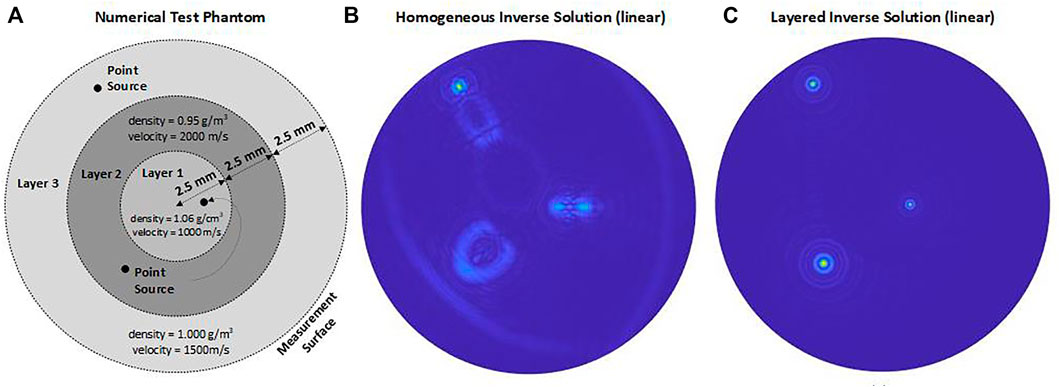
FIGURE 2. (A): Test phantom (B): Numerical simulation obtained under homogeneous medium assumption (C): Numerical simulation obtained for layered medium, showing correct source locations.

FIGURE 3

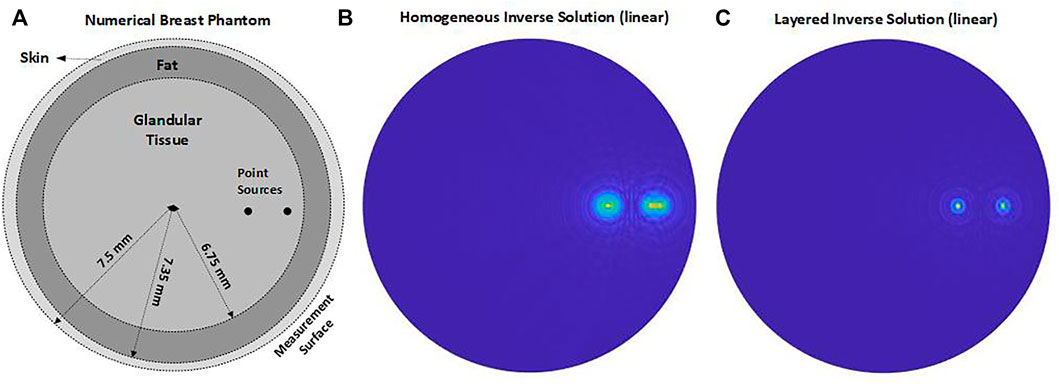
FIGURE 3. (A): Breast phantom (B): Numerical simulation obtained under homogeneous medium assumption (C): Numerical simulation obtained for layered medium, showing correct source locations.

We also test our inverse solution for the capability in measuring the strength of sources by using same layer properties, frequency band and sampling rates with above simulation. We locate two point sources at coordinates (1.25 mm, 0) and (1.25 mm, π) with amplitude values 1 and 10, respectively. In the simulations, again, we generate synthetic data by using layered medium Green’s function in forward solution Eq. 22 of thermoacoustic wave equation and reconstruct the thermoacoustic source distribution from this data using layered inverse solution Eq. 28 including layered medium Green’s functions. The test phantom and numerical simulation results are depicted in Figure 4. Simulation results shows the inverse solution is accurate in distinguishing different source strengths.

FIGURE 4

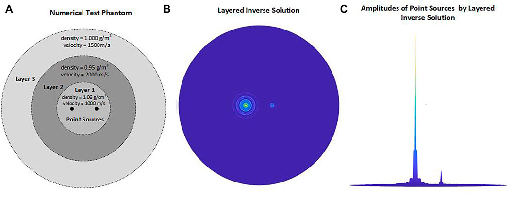
FIGURE 4. (A): Test phantom (B): Numerical simulation obtained by layered medium inverse solution (C): Numerical simulation obtained for layered medium, showing correct source locations.

The limitation of the proposed inverse solution for thermoacoustic imaging is need of tissue properties and structures as apriori information. But, these informations can be obtained from acquired thermoacoustic data or additional transmission ultrasound scan. The error in apriori information of tissue structures will reduce the image quality but this effect can be minimized by some iterative methods.

7 Conclusion

In this study, we have considered the inverse source problem for thermoacoustic wave equation in layered cylindrical models. We have derived an exact analytic inverse solution in frequency domain under boundary conditions. Also, the derived solution was tested in a three-layer numerical tissue models. The solution presented here is a suitable approach for cross-sectional imaging of cylindrical and spherical structures (such as the breast and brain) to get better image quality.

Data Availability Statement

The original contributions presented in the study are included in the article/Supplementary Material, further inquiries can be directed to the corresponding author.

Author Contributions

DE and BÜU did mathematical analysis, derivations and computations of this work. DE did the numerical simulations. DE and BÜU contributed to manuscript revision, read, and approved the submitted version.

Funding

This work was supported by TUBITAK of Turkey through ARDEB-1003 Program under Grant 213E038.

Conflict of Interest

The authors declare that the research was conducted in the absence of any commercial or financial relationships that could be construed as a potential conflict of interest.

Publisher’s Note

All claims expressed in this article are solely those of the authors and do not necessarily represent those of their affiliated organizations, or those of the publisher, the editors and the reviewers. Any product that may be evaluated in this article, or claim that may be made by its manufacturer, is not guaranteed or endorsed by the publisher.

Acknowledgments

We express deep gratitude to Prof. Dr. Mustafa Karaman, who unfortunately passed away, for his contribution to this research by his extensive knowledge and enlightening vision. Previously, outline of this work has been presented as conference paper [17].

Supplementary Material

The Supplementary Material for this article can be found online at: https://www.frontiersin.org/articles/10.3389/fphy.2022.736555/full#supplementary-material

References

1. Idemen M, Alkumru A. On an Inverse Source Problem Connected with Photo-Acoustic and Thermo-Acoustic Tomographies. Wave Motion (2012) 49:595–604. doi:10.1016/j.wavemoti.2012.03.004

CrossRef Full Text | Google Scholar

2. Xu M, Wang LV. Universal Back-Projection Algorithm for Photoacoustic Computed Tomography. Phys Rev E (2005) 71:016706–10167067. doi:10.1103/PhysRevE.71.016706

CrossRef Full Text | Google Scholar

3. Wang LV, Yang X. Boundary Conditions in Photoacoustic Tomography and Image Reconstruction. J Biomed Opt (2007) 12:014027–101402710. doi:10.1117/1.2709861

PubMed Abstract | CrossRef Full Text | Google Scholar

4. Schoonover RW, Anastasio MA. Image Reconstruction in Photoacoustic Tomography Involving Layered Acoustic media. J Opt Soc Am A (2011) 28:1114–20. doi:10.1364/JOSAA.28.001114

CrossRef Full Text | Google Scholar

5. Yuan Xu Y, Wang LV. Effects of Acoustic Heterogeneity in Breast Thermoacoustic Tomography. IEEE Trans Ultrason Ferroelect., Freq Contr (2003) 50:1134–46. doi:10.1109/TUFFC.2003.1235325

CrossRef Full Text | Google Scholar

6. Wang J, Zhao Z, Song J, Chen G, Nie Z, Liu Q-H. Reducing the Effects of Acoustic Heterogeneity with an Iterative Reconstruction Method from Experimental Data in Microwave Induced Thermoacoustic Tomography. Med Phys (2015) 42:2103–12. doi:10.1118/1.4916660

PubMed Abstract | CrossRef Full Text | Google Scholar

7. Wang B, Zhao Z, Liu S, Nie Z, Liu Q. Mitigating Acoustic Heterogeneous Effects in Microwave-Induced Breast Thermoacoustic Tomography Using Multi-Physical K-Means Clustering. Appl Phys Lett (2017) 111:223701. doi:10.1063/1.5008839

CrossRef Full Text | Google Scholar

8. Liu S, Lu Y, Zhu X, Jin H. Measurement Matrix Uncertainty Model-Based Microwave Induced Thermoacoustic Sparse Reconstruction in Acoustically Heterogeneous media. Appl Phys Lett (2021) 119:263701. doi:10.1063/5.0076449

CrossRef Full Text | Google Scholar

9. Ammari H. An Introduction to Mathematics of Emerging Biomedical Imaging. Berlin: Springer (2008).

Google Scholar

10. Colton D, Kress R. Inverse Acoustic and Electromagnetic Scattering Theory. New York: Springer (2013).

Google Scholar

11. Kruger RA, Kiser WL, Miller KD, Reynolds HE, Reinecke DR, Kruger GA, et al. Thermoacoustic Ct: Imaging Principles. In: Proc. SPIE 3916, Biomedical Optoacoustics (2000), 150–159. doi:10.1117/12.386316

CrossRef Full Text | Google Scholar

12. Kuchment P, Kunyansky L. Mathematics of Thermoacoustic Tomography. Eur J Appl Math (2008) 19:191–224. doi:10.1017/S0956792508007353

CrossRef Full Text | Google Scholar

13. Xu M, Wang LV. Photoacoustic Imaging in Biomedicine. Rev Scientific Instr (2006) 77:041101–104110122. doi:10.1063/1.2195024

CrossRef Full Text | Google Scholar

14. Arfken GB, Weber HJ. Mathematical Methods for Physicists. Newyork: Academic Press (1995).

Google Scholar

15. Stakgold I. Green’s Function and Boundary Value Problems. New York: Wiley (1979).

Google Scholar

16. Kinsler LE, Frey AR, Coppens AB, Sanders JV. Fundamentals of Acoustics. New York: Wiley (1982).

Google Scholar

17. Elmas D, Uzun B, İdemen M, Karaman M. Inverse Solution of Thermoacustic Wave Equation for Cylindirical Multi-Layer Mediums, In 25th Signal Processing and Communications Applications Conference, SIU 2017. IEEE (2017). doi:10.1109/siu.2017.7960734

CrossRef Full Text | Google Scholar