 Ruiling Wang
 Yakui Xue1*
- 1School of Mathematics, North University of China, Taiyuan, China
- 2Department of Mathematics, University of South Australia, Adelaide, Australia
In order to prevent the propagation of computer worms effectively, based on the latent character of worms, the exposed compartments of computer and USB device are introduced respectively, and a series of computer worm propagation models with saturation incidence rate are proposed. The qualitative behavior of the proposed model is studied. Firstly, the threshold R0 of the model is derived by using the next-generation matrix method, which completely characterized the stability of disease free equilibrium and endemic equilibrium. If R0 < 1, the disease free equilibrium is asymptotically stable, implying that the worm dies out eventually and its attack remains under control; if R0 > 1, the asymptotic stability of endemic equilibrium under certain conditions is proved, which means that the worm is always persistent and uncontrollable under such conditions. Secondly, the theoretical results are verified by numerical study, in which the relative importance of each parameter in worm prevalence is evaluated by sensitivity analysis. Finally, so as to minimize the number of computer and USB device carrying computer worms in short span of time, the worm propagation model is extended to incorporate three control strategies. The Pontryagin’s maximum principle is used to characterize the controls’ optimal levels. According to the control effect diagram, the combined strategy is effective in minimizing the transmission dynamics of worm virus in computer and USB devices populations respectively.
1 Introduction
As a storage medium, USB device is favored by many office workers because of its large storage capacity and portability. It is often used to copy data between different computers. In fact, the transmission of data via USB device may be accompanied by the spread of worms [1]. Computer worm is a common computer virus, which has the characteristics of wide spread and serious harm [2]. On 13 January 2021, the news of incaseformat worm flooded wechat circle of friends, and infection cases were found in many provinces, cities, and industries, with a trend of large-scale outbreak. After execution, the worm will automatically copy to the windows directory of the system disk and create a registry to start itself [3]. Once the user restarts the computer, this will cause the worm host to execute from the windows directory, and then the worm process will traverse all disks except the system disk and delete the files, causing irreparable losses to the user. Therefore, it has become an urgent problem in the field of network security to study the propagation rule of computer worm and effectively control its propagation.
A computer worm is a group of programmed code that can reproduce itself and affect the normal use of the computer [4]. A biological virus is a unique tiny living organism, which can make use of the nutrients of the host cell to copy its own essential constituent material DNA or RNA and proteins [5–7]. Computer worms and biological viruses are two concepts from different fields, but some of their properties have striking similarities [8]. Mainly in the following four aspects: firstly, computer worms and biological viruses are infectious. Computer worms can spread from an infected computer to an uninfected computer through network or other remavable devices. Biological viruses can also be transmitted by direct or indirect contact between living organisms. Then, computer worms and biological viruses are latent and generally not easy to find. Computer worms can integrate their own program fragments into the system programs, so that their most important code can be saved from the anti-virus software. Biological viruses can also integrate their genetic material into the host’s DNA or RNA, thereby escaping attack by the host’s immune system. In addition, computer worms and biological viruses will mutate in the process of spreading, making their species more and more diverse. Finally, both computer worms and biological viruses are destructive. Computer worms can damage the computer system and interfere with the normal operation of the computer. Biological viruses may damage the cells or organs of the host organism, which may pose a threat to the organism’s life. Because of the high similarity between computer worms and biological viruses, we used the method of studying the transmission of infectious diseases to explore the dynamic behavior of computer worms.
In epidemiology, dynamic model has been an important method in analysing the spread and control of infectious diseases qualitatively and quantitatively [9–11]. In 1991, Kephart and White first introduced the dynamic model of infectious disease into the study of the propagation of computer virus. Since then, the dynamic model has also become a vital tool for the study of various computer viruses [12–16]. The research on computer worms have experienced a rapid growth, and a large number of models have been established, mathematically analyzed, which provides some useful and valid references for the characteristics of computer worms transmission [17]. In 2011, Song et al. [18] studied removable device as an independent carrier for the first time. They hypothesized that computer worms spread via both web-based scanning and removable devices, established SIR model of computer population and SI model of removable devices population, studied their dynamic behavior, and gave corresponding control strategy. In 2012, Zhu et al. [19] proposed a new dynamic model to describe the spread of computer virus by using the same method as in Ref. [18]. In addition, by qualitative analysis, it is concluded that controlling R0 below one is an effective means to extinguish virus, which provides a good start point for understanding the transmission of computer virus through such interactions. In 2015, Ma et al. [20] proposed SIBV model of fixed nodes and SI model of mobile nodes considering the influence of benign worms and mobile devices in the network environment, discussed the influences of removable devices on the interaction dynamics between malicious worms and benign worms. Through numerical analysis and simulation, it is proved that the anti-worm technology can effectively suppress the spread of malicious worms. In 2018, Zhu et al. [21] introduced two control strategies of disconnecting computers from removable devices and reorganizing computers on the basis of Ref. [19], and studied the optimal control of virus transmission between computers and removable devices. Different from previous studies, this paper does not use a fixed cost weight index in the objective function, but uses a state-based cost weight index. In 2020, Kim et al. [1] proposed and analyzed a scheme to control virus transmission through vaccination, that is, installing effective anti-virus software. The results showed that the higher the vaccination rate, the lower the number of infected computers.
Inspired by the models above, we establish a new worm transmission model. We adopt the saturation incidence rate [22, 23], which can present the inhibition effect of susceptible devices and the crowding effect of infectious devices and can also ensure the boundness of contact rate by choosing suitable parameters [24]. In addition, considering the latent character of computer worms, the exposed compartments of computer and USB are introduced [25–28]. The rest of the article is organized as follows: in Section 2, qualitative analysis of the dynamical system is carried out, and sufficient conditions for the existence of equilibria and asymptotic stability are given; numerical findings and discussion are conducted in Section 3; in Section 4, optimal control strategy is proposed; and conclusion is presented in Section 5.
2 Dynamical model
The main purpose of this paper is to explore the dynamic behavior of computer worms transmission in the process of using USB devices to transmit data, so as to formulate effective strategies to control the spread of worms. This model is an improved version of Kim et al. [1]. In this model, the computer acts as the host and the USB device acts as a vector. Among them, the total computer population is divided into the following four subclasses, which are Sc(t), Ec(t), Ic(t), and Rc(t), representing the numbers of susceptible computers, exposed computers, infectious computers and recovered computers at time t. And similarly for USB devices population, which is classified into three vector population subclasses, namely Su(t), Eu(t), and Iu(t), represent the numbers of susceptible USB devices, exposed USB devices and infectious USB devices at time t, respectively. In addition, the following model assumptions are presented:
(H1) All newly launched computers and removable USB devices are susceptible.
(H2) At time t, the infectious force of infected USB devices to susceptible computers is given by
(H3) Infected computers will gain temporary immunity after recovery due to anti-virus software installed, but after a period of time will join again susceptible class because of the variability of computer worms.
(H4) Computer dysfunction is not only related to natural death, but also to worm invasion.
The improved model as follow:
For the computer population in system (Eq. 1), Λ1 is the recruitment rate of computer population; σ is the efficiency coefficient of the anti-virus software; ν is installation coverage rate coefficient of anti-virus software; β1 is infection rate coefficient of susceptible computers by infectious USB devices; α1 is the degree coefficient of protection measures taken for susceptible computers in case of worms outbreak; μ1 is the natural elimination rate coefficient of computer population; θ is the elimination rate coefficient of computer population caused by worm invasion; τ, η, ϵ, γ are the transition rate coefficients among states in the computer population.
As for the USB population in system (Eq. 1), Λ2 is the recruitment rate of USB population; β2 is infection rate coefficient of susceptible USB devices by infectious computers; α2 is the degree coefficient of protection measures taken for susceptible USB devices in case of worms outbreak; μ2 is the natural elimination rate coefficient of USB population; ϕ, p, ξ are the transition rate coefficients among states in the USB population.
Suppose Nc and Nu are the total number of computer population and USB population at time t, respectively, satisfying Nc = Sc + Ec + Ic + Rc and Nu = Su + Eu + Iu. Add the equations in system (Eq. 1) to get
In this section, we firstly prove the existence of disease free equilibrium and endemic equilibrium of system (Eq. 1), and obtain the basic reproduction number R0 through calculation which determines the propagation dynamics of system (Eq. 1). Secondly, we provide the local and global stability of disease free equilibrium and endemic equilibrium under certain conditions, which establishes the theoretical foundation for the control strategies of worm attack.
2.1 Existence of basic reproduction number and equilibria
Our aim is to study the characteristics of disease free equilibrium and endemic equilibrium. Let the right-hand side of system (Eq. 1) equals zero, and the disease free equilibrium can be obtained:
Next, we calculate the basic reproduction number R0, which is essentially the number of secondary infectious cases produced in a susceptible class by a single infectious node in its overall infectious duration. This is a decisive threshold in epidemiological systems that can be used to predict whether computers will be continuously attacked by worms [29]. According to the next-generation matrix method in literature [30], we have the following:
Thus, we obtain the basic reproduction number:
Theorem 1 When R0 > 1, system (Eq. 1) has a unique endemic equilibrium.
Proof: Make the right side of system (Eq. 1) equal to zero, and substitute the endemic equilibrium
We get the expression
When R0 > 1, b < 0, so
2.2 Stability of disease free equilibrium
In this subsection, we analyze the asymptotical stability of disease free equilibrium P0.
Theorem 2 The disease free equilibrium P0 of system (Eq. 1) is locally asymptotically stable if R0 < 1 and is unstable if R0 > 1.
Proof: The Jacobian matrix of system (Eq. 1) at P0 is
where
By elementary row operations, we get
where
When
Theorem 3 The disease free equilibrium P0 of system (Eq. 1) is globally asymptotically stable in region Δ if R0 < 1 and is unstable if R0 > 1.
Proof: The Castillo-Chavez method in Refs. [31] is used to prove it. First, let χ1 = (Sc, Rc, Su), χ2 = (Ec, Ic, Eu, Iu) and define
We decompose system (Eq. 1) into two subsystems,
where
Because
According to (Eq. 10), when t → ∞,
Moreover, it is obvious that
The population limits of computer and USB device are
2.3 Stability of endemic equilibrium
In this subsection, we analyze the asymptotical stability of endemic equilibrium P*.
Theorem 4 The endemic equilibrium P* of system Eq. 1 is locally asymptotically stable if
Proof: The Jacobian matrix of system (Eq. 1) at P* is given by
where
After simplification we get
where
It is obvious that a22, a33, a66, c11, c55 < 0, and then, d22, d33, d44, d66 < 0 can be obtained according to the above expressions. Besides, when
Next, the geometrical approach in Refs. [33] is used to determine the condition that system (Eq. 1) achieves global asymptotic stability at the endemic equilibrium.
Theorem 5 If
Proof: We prove the global stability of endemic equilibrium P∗ under the above conditions by using geometrical approach [32, 34, 35], which is the generalization of Lyapunov theory in essence, by using the third additive compound matrix. Consider the subsystems of system (Eq. 1)
Let J be the Jacobian matrix of system (Eq. 14) given by
Based on [35], the third additive compound matrix of J is denoted by
where
Now let us choose a function
Therefore,
and
So that
where
Consequently, if
and if
Similarly,
and if
If
Thus, combining the above four inequalities, we get the following inequality:
This shows that the subsystem of system (Eq. 1) containing four non-linear differential equations is globally asymptotically stable around the equilibrium
3 Numerical simulation
In this section, we refer to the data of Refs. [36–38] to analyze the performance and dynamic behavior of the studied model through numerical simulation, and demonstrate the feasibility of the theoretical results obtained.
3.1 Stability of equilibria
The stability of disease free equilibrium and endemic equilibrium of system (Eq. 1) is verified by numerical simulation. Figure 1 and Figure 2 show the stability simulation diagram of disease free equilibrium and endemic equilibrium. Initially the number of susceptible computers, exposed computers, infected computers, recovery computers, susceptible USB devices, exposed USB devices and infected USB devices are Sc(0) = 50,000, Ec (0) = 20,000, Ic(0) = 10,000, Rc (0) = 10,000, Su(0) = 5,000, Eu (0) = 3,000, and Iu(0) = 1,000, separately. We take the parameters Λ1 = 0.75, Λ2 = 0.1, σ = 0.6, ν = 0.1, β1 = 0.035, β2 = 0.035, α1 = 0.8, α2 = 0.3, μ1 = 0.1, μ2 = 0.1, τ = 0.1, η = 0.45, ϵ = 0.25, ϕ = 0.05, p = 0.003, ξ = 0.005, θ = 0.001, γ = 0.05, at which time, R0 ≈ 0.0039 < 1. It can be seen from Figure 1 that the number of exposed computers Ec, infected computers Ic, exposed USB devices Eu and infected USB devices Iu gradually approach zero, which shows the correctness of Theorem 2 and Theorem 3. When β1 = 0.053, μ1 = 0.01, ξ = 0.05, and other parameters remain unchanged, R0 ≈ 1.0670 > 1. Compared with Figure 1, the number of exposed computers Ec, infected computers Ic, exposed USB devices Eu and infected USB devices Iu in Figure 2 are not zero and reach a stable value, which is also consistent with Theorems 4 and 5.
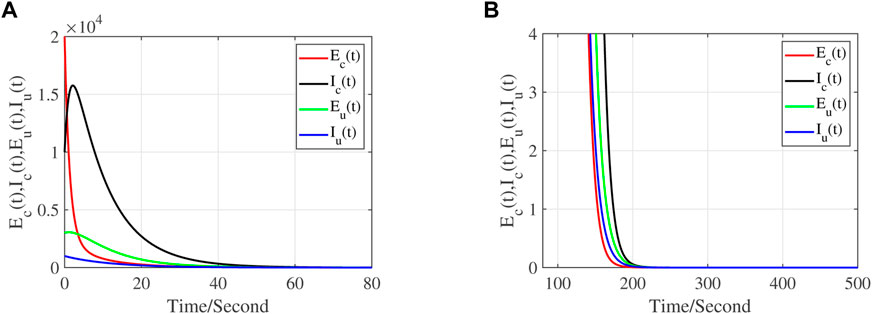
FIGURE 1. Time series plot of system (1) with Λ1 = 0.75, Λ2 = 0.1, σ = 0.6, ν = 0.1, β1 = 0.035, β2 = 0.035, α1 = 0.8, α2 = 0.3, μ1 = 0.1, μ2 = 0.1, τ = 0.1, η = 0.45, ϵ = 0.25, ϕ = 0.05, p = 0.003, ξ = 0.005, θ = 0.001, γ = 0.05. (A) the tendency of the worm propagation in a short period, (B) the tendency of the worm propagation in a later period.
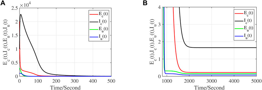
FIGURE 2. Time series plot of system (1) with Λ1 = 0.75, Λ2 = 0.1, σ = 0.6, ν = 0.1, β1 = 0.053, β2 = 0.035, α1 = 0.8, α2 = 0.3, μ1 = 0.01, μ2 = 0.1, τ = 0.1, η = 0.45, ϵ = 0.25, ϕ = 0.05, p = 0.003, ξ = 0.05, θ = 0.001, γ = 0.05. (A) the tendency of the worm propagation in a short period, (B) the tendency of the worm propagation in a later period.
3.2 Performance comparison of the SEIRSEI model with the SIRSI model
To evaluate the performance of the SEIRSEI model, numerical methods are used to compare it with the SIRSI model [1]. We simulate SEIRSEI and SIRSI models by Matlab. Both models share the same parameters as in Section 3.1. Figure 3 shows the number of infected computers and infected USB devices for both models. The results show that, compared with SIRSI model, the propagation speed of worms and the number of infected computers and USB devices in SEIRSEI model are significantly decreased. This implies that the SEIRSEI model takes much smaller time to combat the worm than the SIRSI model. Obviously, the results shown in Figure 3 verify that the proposed model is more effective in controlling computer worms attack than the previous model.
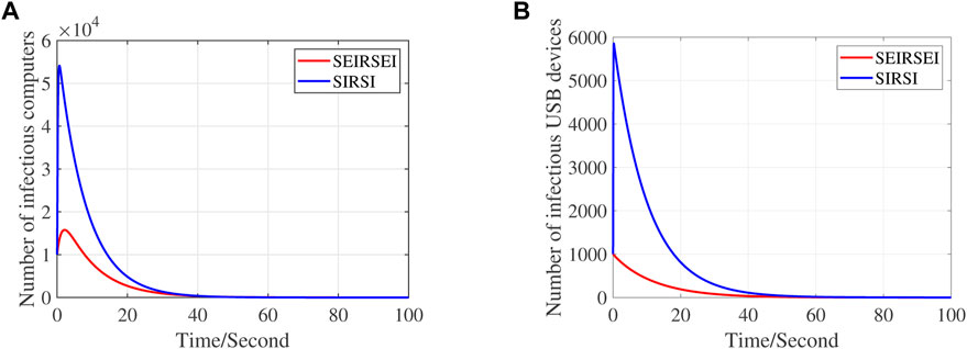
FIGURE 3. Performance comparison of the SEIRSEI model with the SIRSI model. (A) graph of infectious number of computers, (B) graph of infectious number of USB devices.
3.3 Sensitivity analysis
Sensitivity analysis is used to determine which parameters have a significant effect on decreasing the spread of disease. Forward sensitivity analysis is considered an important component of epidemic modeling, although it is tedious to calculate for complex biological models. The ecologist and epidemiologist paid a lot of attention to the sensitivity study of R0.
Definition. The normalized forward sensitivity index of R0 that depends differentiability on a parameter ω is defined as
The following three methods are normally used to calculate the sensitivity indices, (i) by direct differentiation, (ii) by a Latin hypercube sampling method, (iii) by linearizing system (Eq. 1), and then solving the obtain set of linear algebraic equations. We will apply the direct differentiation method as it gives analytical expressions for the indices. The indices not only shows us the influence of various aspects associated with the spreading of infectious disease but also gives us important information regarding the comparative change between R0 and different parameters. Consequently, it helps in developing the control strategies.
Table 1 demonstrates that the parameters Λ1, Λ2, β1, β2, τ, η and ξ have a positive influence on the reproduction number R0, which describe that the growth or decay of these parameters say by 10% will increase or decrease the reproduction number by 10%, 10%, 10%, 10%, 1.1%, 4.3% and 9.6% respectively. But on the other hand, the index for parameters σ, ν, μ1, μ2, ϵ, ϕ, p, θ and γ illustrates that increasing their values by 10% will decrease the values of reproduction number R0 by 2.9%, 2.9%, 16.7%, 26.1%, 3.1%, 3.2%, 0.29%, 0.06%, and 3.3% respectively. α1 and α2 have no impact on the reproduction number R0. Figures 4A–H are plotted to demonstrate the variations in the basic reproductive number R0 with respect to the different model parameters.
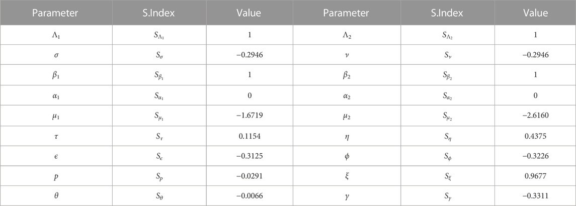
TABLE 1. Sensitivity indices of the basic reproduction number R0 against mentioned parameters.
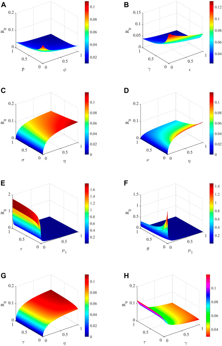
FIGURE 4. Sensitivity analysis of different parameters. (A) R0 versus sensitive parameters p and ϕ, (B) R0 versus sensitive parameters γ and ϵ, (C) R0 versus sensitive parameters σ and η, (D) R0 versus sensitive parameters ν and η, (E) R0 versus sensitive parameters τ and μ1, (F) R0 versus sensitive parameters θ and μ1, (G) R0 versus sensitive parameters τ and η, (H) R0 versus sensitive parameters τ and γ.
4 Optimal control strategy formulation
In order to explore how to effectively control the propagation of computer worms, system (Eq. 1) is improved in this section. Three control variables
Defining the objective function
where A1, A2, A3 and A4 are positive weight constants of Ec, Ic, Eu and Iu respectively, and T is the final time to implement the control strategies.
The control set is defined as
Based on the boundedness of the right end of system (Eq. 21) and the convexity of the integrand of (Eq. 22), the existence of the optimal control
To find the optimal solution of the optimal control problem (Eqs 21, 22), the Hamilton function is defined as follows
where
Theorem 6 Let
where i = Sc, Ec, Ic, Rc, Su, Eu, Iu. In addition, the corresponding optimal control variables
Proof: To prove the theorem, the differential of (Eq. 23), namely the Hamiltonian function H, with respect to the state variables Sc, Ec, Ic, Rc, Su, Eu, Iu are obtained, and the corresponding adjoint system is as follows:
and with transversality conditions
For sufficiently small final time T, the uniqueness of the optimal control of the system has been achieved owing to the boundedness of the state variables and adjoint variables together with the Lipschitz property of systems (Eq. 21) and (Eq. 26).
In order to show the rationality and effectiveness of the control strategy mentioned in Section 4, numerical simulation is carried out. Figure 5 shows a substantial decrease in the population of exposed computers, infected computers, exposed USB devices and infected USB devices respectively relative to the case of no control, when the combined strategy is implemented, including the installation coverage rate of anti-virus software and the disinfection of computer and USB device. Parameter Λ1 = 0.75, Λ2 = 0.1, σ = 0.6, ν = 0.1, β1 = 0.035, β2 = 0.035, α1 = 0.8, α2 = 0.3, μ1 = 0.1, μ2 = 0.1, τ = 0.1, η = 0.45, ϵ = 0.25, ϕ = 0.05, p = 0.003, ξ = 0.005, θ = 0.001, γ = 0.05. We draw the conclusion that the spread of worm virus can be effectively controlled by strengthening users’ computer security education, improving their understanding of anti-virus software, and calling on users to disinfect computers and USB devices regularly.
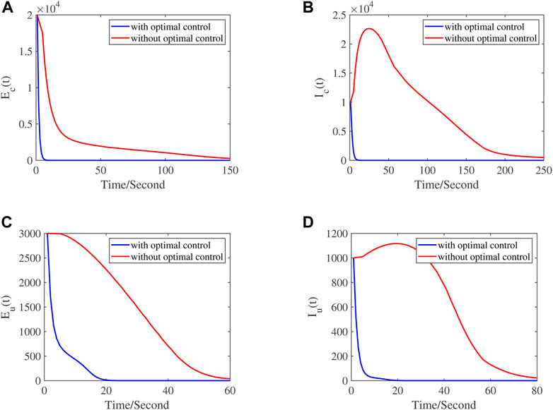
FIGURE 5. Plots of different classes showing the difference between with control and without control, respectively: (A) exposed computers, (B) infected computers, (C) exposed USB devices, (D) infected USB devices.
5 Conclusion and discussion
This paper mainly considers the dynamic behavior of computer worms in the process of using USB to transmit data. The novel ideas of our paper are as follows: (a) the exposed compartments of computer and USB are introduced because of the latent nature of worms; (b) infected computers will gain temporary immunity after recovery due to anti-virus software installed, but after a period of time will join again susceptible class because of the variability of computer worms; (c) the elimination rate of computers is not only related to natural mortality, but also to worm attacks; (d) the saturation incidence is used thanks to the inhibition effect of susceptible equipments and the crowding effect of infectious equipments.
Firstly, through theoretical analysis, the existence of disease free equilibrium and endemic equilibrium is studied, and the sufficient conditions for their asymptotic stability are given. The global stability of disease free equilibrium is carried out using the Castillo-Chavez method, whereas, the global stability of the unique endemic equilibrium is also investigated via using geometrical approach. It can be seen that when R0 < 1, worm transmission is effectively controlled and verified by numerical simulation. Therefore, one effective means to extinguish worm is to keep R0 below 1. Furthermore, the sensitivity analysis is complemented by numerical simulation to explore the influence of some parameter changes on the basic reproduction number R0. It is seen that Λ1, Λ2, β1, β2, τ, η and ξ are positively correlated with R0, while σ, ν, μ1, μ2, ϵ, ϕ, p, θ and γ are negatively correlated with R0. Finally, we establish a optimal control system by taking the installation coverage rate of anti-virus software and the disinfection of computer and USB device as control variables. The numerical simulation results show that compared with the situation without control measures, the total number of computers and USB devices in the exposed state and infected state is significantly reduced after control measures are taken, that is to say, adding control could effectively reduce the spread of computer worms.
In this paper, the mathematical model is used to describe the propagation process of computer worms, which is helpful to analyze the propagation characteristics of worms, and then propose more effective defense measures and control strategies. In addition, the research of this subject is beneficial to predict the propagation trend of worms, test the effect of various defensive measures, and provide theoretical guidance for the defense and control of computer worms.
Data availability statement
The original contributions presented in the study are included in the article/Supplementary Material, further inquiries can be directed to the corresponding author.
Author contributions
RW, YX, and KX conceived the study. RW developed the mathematical model, computations, simulation coding, manuscript writing and data interpretation. YX contributed to supervision and validation. KX performed literature survey and computations. All authors contributed to the article and approved the submitted version.
Funding
This work was supported by the National Natural Science Foundation of China (grant number 11971278); the Shanxi Scholarship Council of China (grant number 2022-150) and Natural Science Foundation of Shanxi Province (grant number 202203021211086).
Conflict of interest
The authors declare that the research was conducted in the absence of any commercial or financial relationships that could be construed as a potential conflict of interest.
Publisher’s note
All claims expressed in this article are solely those of the authors and do not necessarily represent those of their affiliated organizations, or those of the publisher, the editors and the reviewers. Any product that may be evaluated in this article, or claim that may be made by its manufacturer, is not guaranteed or endorsed by the publisher.
References
1. Kim KS, Ibrahim MM, Jung IH, Kim S. Mathematical analysis of the effectiveness of control strategies to prevent the autorun virus transmission propagation. Appl Maths Comput (2020) 371:124955. doi:10.1016/j.amc.2019.124955
2. Deng Y, Pei Y, Li C. Parameter estimation of a susceptible–infected–recovered–dead computer worm model. SIMULATION (2022) 98:209–20. doi:10.1177/00375497211009576
3. Piqueira JRC, Cabrera MA, Batistela CM. Malware propagation in clustered computer networks. Physica A: Stat Mech its Appl (2021) 573:125958. doi:10.1016/j.physa.2021.125958
4. Xiao X, Fu P, Dou C, Li Q, Hu G, Xia S. Design and analysis of seiqr worm propagation model in mobile internet. Commun nonlinear Sci Numer simulation (2017) 43:341–50. doi:10.1016/j.cnsns.2016.07.012
5. Zheng W, Wang T, Liu C, Yan Q, Zhan S, Li G, et al. Liver transcriptomics reveals microrna features of the host response in a mouse model of dengue virus infection. Comput Biol Med (2022) 106057:106057. doi:10.1016/j.compbiomed.2022.106057
6. Carrillo M, Góngora PA, Rosenblueth DA. An overview of existing modeling tools making use of model checking in the analysis of biochemical networks. Front Plant Sci (2012) 3:155. doi:10.3389/fpls.2012.00155
7. Yang G, Gómez Tejeda Zañudo J, Albert R. Target control in logical models using the domain of influence of nodes. Front Physiol (2018) 454:454. doi:10.3389/fphys.2018.00454
8. Ren J, Xu Y. A compartmental model for computer virus propagation with kill signals. Physica A: Stat Mech its Appl (2017) 486:446–54. doi:10.1016/j.physa.2017.05.038
9. Razzaq OA, Khan NA, Faizan M, Ara A, Ullah S. Behavioral response of population on transmissibility and saturation incidence of deadly pandemic through fractional order dynamical system. Results Phys (2021) 26:104438. doi:10.1016/j.rinp.2021.104438
10. Paul AK, Kuddus MA. Mathematical analysis of a Covid-19 model with double dose vaccination in Bangladesh. Results Phys (2022) 35:105392. doi:10.1016/j.rinp.2022.105392
11. Tiwari V, Deyal N, Bisht NS. Mathematical modeling based study and prediction of Covid-19 epidemic dissemination under the impact of lockdown in India. Front Phys (2020) 8:586899. doi:10.3389/fphy.2020.586899
12. Toutonji O, Yoo S-M. Passive benign worm propagation modeling with dynamic quarantine defense. KSII Trans Internet Inf Syst (Tiis) (2009) 3:96–107. doi:10.3837/tiis.2009.01.005
13. Wang F, Zhang Y, Wang C, Ma J, Moon S. Stability analysis of a seiqv epidemic model for rapid spreading worms. Comput Security (2010) 29:410–8. doi:10.1016/j.cose.2009.10.002
14. Yao Y, Xie X-w., Guo H, Yu G, Gao F-X, Tong X-j. Hopf bifurcation in an internet worm propagation model with time delay in quarantine. Math Comput Model (2013) 57:2635–46. doi:10.1016/j.mcm.2011.06.044
15. Zhou P, Gu X, Nepal S, Zhou J. Modeling social worm propagation for advanced persistent threats. Comput Security (2021) 108:102321. doi:10.1016/j.cose.2021.102321
16. Yang L-X, Yang X. The impact of nonlinear infection rate on the spread of computer virus. Nonlinear Dyn (2015) 82:85–95. doi:10.1007/s11071-015-2140-z
17. Zhang Z, Zou J, Upadhyay RK, ur Rahman G. An epidemic model with multiple delays for the propagation of worms in wireless sensor networks. Results Phys (2020) 19:103424. doi:10.1016/j.rinp.2020.103424
18. Song L-P, Jin Z, Sun G-Q, Zhang J, Han X. Influence of removable devices on computer worms: Dynamic analysis and control strategies. Comput Maths Appl (2011) 61:1823–9. doi:10.1016/j.camwa.2011.02.010
19. Zhu Q, Yang X, Ren J. Modeling and analysis of the spread of computer virus. Commun Nonlinear Sci Numer Simulation (2012) 17:5117–24. doi:10.1016/j.cnsns.2012.05.030
20. Ma J, Chen Z, Wu W, Zheng R, Liu J. Influences of removable devices on the anti-threat model: Dynamic analysis and control strategies. Information (2015) 6:536–49. doi:10.3390/info6030536
21. Zhu Q, Loke SW, Zhang Y. State-based switching for optimal control of computer virus propagation with external device blocking. Security and Communication Networks (2018). doi:10.1155/2018/4982523
22. Upadhyay RK, Kumari S. Detecting malicious chaotic signals in wireless sensor network. Physica A: Stat Mech its Appl (2018) 492:1129–52. doi:10.1016/j.physa.2017.11.043
23. Gao Q, Zhuang J. Stability analysis and control strategies for worm attack in mobile networks via a veiqs propagation model. Appl Maths Comput (2020) 368:124584. doi:10.1016/j.amc.2019.124584
24. Hu R, Gao Q, Wang B. Dynamics and control of worm epidemic based on mobile networks by seiqr-type model with saturated incidence rate. Discrete Dyn Nat Soc (2021) 2021:1–22. doi:10.1155/2021/6637263
25. Madhusudanan V, Srinivas M, Nwokoye CH, Murthy BN, Sridhar S. Hopf-bifurcation analysis of delayed computer virus model with holling type iii incidence function and treatment. Scientific Afr (2022) 15:e01125. doi:10.1016/j.sciaf.2022.e01125
26. Mishra BK, Pandey SK. Dynamic model of worm propagation in computer network. Appl Math Model (2014) 38:2173–9. doi:10.1016/j.apm.2013.10.046
27. Mishra BK, Pandey SK. Dynamic model of worms with vertical transmission in computer network. Appl Math Comput (2011) 217:8438–46. doi:10.1016/j.amc.2011.03.041
28. Guillén JH, Del Rey AM, Encinas LH. Study of the stability of a seirs model for computer worm propagation. Physica A: Stat Mech its Appl (2017) 479:411–21. doi:10.1016/j.physa.2017.03.023
29. Upadhyay RK, Singh P. Modeling and control of computer virus attack on a targeted network. Physica A: Stat Mech its Appl (2020) 538:122617. doi:10.1016/j.physa.2019.122617
30. Van den Driessche P, Watmough J. Reproduction numbers and sub-threshold endemic equilibria for compartmental models of disease transmission. Math biosciences (2002) 180:29–48. doi:10.1016/S0025-5564(02)00108-6
31. Castillo-Chavez C, Blower S, Van den Driessche P, Kirschner D, Yakubu A-A. Mathematical approaches for emerging and reemerging infectious diseases: Models, methods, and theory, 126. Springer Science & Business Media (2002).
32. Khan A, Zarin R, Inc M, Zaman G, Almohsen B. Stability analysis of leishmania epidemic model with harmonic mean type incidence rate. The Eur Phys J Plus (2020) 135:528–0. doi:10.1140/epjp/s13360-020-00535-0
33. Li MY, Muldowney JS. A geometric approach to global-stability problems. SIAM J Math Anal (1996) 27:1070–83. doi:10.1137/S0036141094266449
34. Khan K, Zarin R, Khan A, Yusuf A, Al-Shomrani M, Ullah A. Stability analysis of five-grade leishmania epidemic model with harmonic mean-type incidence rate. Adv Difference Equations (2021) 2021:86–27. doi:10.1186/s13662-021-03249-4
35. Khan A, Zarin R, Ahmed I, Yusuf A, Humphries UW. Numerical and theoretical analysis of rabies model under the harmonic mean type incidence rate. Results Phys (2021) 29:104652. doi:10.1016/j.rinp.2021.104652
36. Yang F, Zhang Z, Zeb A. Hopf bifurcation of a veiqs worm propagation model in mobile networks with two delays. Alexandria Eng J (2021) 60:5105–14. doi:10.1016/j.aej.2021.03.055
37. Haldar K, Mishra BK. A mathematical model for a distributed attack on targeted resources in a computer network. Commun Nonlinear Sci Numer Simulation (2014) 19:3149–60. doi:10.1016/j.cnsns.2014.01.028
38. Khanh NH, Huy NB. Stability analysis of a computer virus propagation model with antidote in vulnerable system. Acta Mathematica Scientia (2016) 36:49–61. doi:10.1016/S0252-9602(15)30077-1
39. Alexander ME, Moghadas SM, Röst G, Wu J. A delay differential model for pandemic influenza with antiviral treatment. Bull Math Biol (2008) 70:382–97. doi:10.1007/s11538-007-9257-2
Keywords: computer worms, saturation incidence rate, stability analysis, sensitivity analysis, optimal control, numerical simulation
Citation: Wang R, Xue Y and Xue K (2023) Dynamic analysis and optimal control of worm propagation model with saturated incidence rate. Front. Phys. 10:1098040. doi: 10.3389/fphy.2022.1098040
Received: 14 November 2022; Accepted: 09 December 2022;
Published: 10 January 2023.
Edited by:
Xiaoming Zheng, Central Michigan University, United StatesReviewed by:
Zizhen Zhang, Anhui University of Finance and Economics, ChinaXue Ren, Harbin Engineering University, China
Copyright © 2023 Wang, Xue and Xue. This is an open-access article distributed under the terms of the Creative Commons Attribution License (CC BY). The use, distribution or reproduction in other forums is permitted, provided the original author(s) and the copyright owner(s) are credited and that the original publication in this journal is cited, in accordance with accepted academic practice. No use, distribution or reproduction is permitted which does not comply with these terms.
*Correspondence: Yakui Xue, eHlrNTE1MkAxNjMuY29t