Defect identification in adhesive structures using multi-Feature fusion convolutional neural network

The interface-debonding defects of adhesive bonding structures may cause a reduction in bonding strength, which in turn affects the bonding quality of adhesive bonding samples. Hence, defect recognition in adhesive bonding structures is particularly important. In this study, a terahertz (THz) wave was used to analyze bonded structure samples, and a multi-feature fusion convolutional neural network (CNN) was used to identify the defect waveforms. The pooling method of the squeeze-and-excitation (SE) attention mechanism was optimized, defect feature weights were adaptively assigned, and feature fusion was conducted using automatic label net-works to segment the THz waveforms in the adhesive bonding area with fine granularity waveforms as an input to the multi-channel CNN. The results revealed that the speed of the THz waveform labeling with the automatic labeling network was 10 times higher than that with traditional methods, and the defect-recognition accuracy of the defect-recognition network constructed in this study was up to 99.28%. The F1-score was 99.73%, and the lowest pre-embedded defect recognition error rate of the generalization experiment samples was 0.27%.

1 Introduction

Adhesive bonding, one of the main connection methods of composite materials, has significant advantages over traditional mechanical fastening technologies, such as reducing structure weight, diminishing stress concentration, and ensuring structural integ-rity [1]. When applying composite adhesive bonding structures [2], the material can undergo easy aging, resulting in a decline in bonding strength, which inevitably causes defects such as matrix cracking and interface debonding. The size of defects varies from several microns to several centimeters [3, 4]. Because interface debonding defects are hidden inside the bonded structure sample, it is difficult to identify them.

The adhesive bonding structure of ceramic matrix composites (CMCs) [5] (hereinafter referred to as adhesive bonding structure), which is generally composed of CMC, adhesive bonding layer I (adhesive layer I), cushion, adhesive bonding layer II (adhesive layer II), and a metal plate, was used as an example in this study. Terahertz (THz) waves are usually used to detect bonding defects in adhesive bonding structures [6–8] owing to the unique physical features of CMCs. Zhang et al. [9] successfully established a method for detecting defects using THz detection data of an adhesive bonding structure by fusion imaging of multiple feature parameters, and the measurement error was 4% when the defect thick-ness was 500 μm, the measurement error is 10.9% when the defect thickness is 200 µm. Wu et al. [10] located the defects by applying the impulse response de-convolution algorithm to THz defect recognition of the adhesive bonding structure. Zhang et al. [11] proposed a defect recognition method for the adhesive bonding structure based on the statistical characteristics of variance and kurtosis, Achieve the minimum detection thickness for layer I is 50 µm and for layer II is 250 μm, respectively. In the abovementioned studies, the waveform features of THz detection were all artificially selected to realize imaging, and subsequently, the defect locations were determined to recognize defects. However, as the thickness of the sample changes, the feature peaks and valleys at the interfaces of different bonding materials change with the location of the time window. This results in the inability to image through a specific time domain interval and the need for human intervention in the location of the feature valleys, which results in a lower recognition efficiency. With the extensive use of bonded structure samples, the amount of data generated by THz non-destructive testing also increases. The traditional defect identification methods have low identification efficiency and are greatly affected by subjective factors, which cannot meet the needs of the rapidly developing THz non-destructive testing industry, an intelligent defect recognition method for adhesive bonding structures is required.

Neural networks have been widely studied in the field of intelligent recognition [12–14]. In the THz domain, an R-pulse coupled neural network model was used to detect objects hidden in the human body based on THz images [15]. The water absorption line in the THz spectra was eliminated through neural network training of the signals collected under different air-humidity levels [16]. Neural networks have been used to analyze and identify the components of transgenic maize [17]. When the microstructure of the thermal barrier coating is uneven due to the imperfect TBC spraying conditions, the long short-term memory (LSTM) network is used to identify the time of flight difference between waveform features, and then measure the thickness of the thermal barrier coating to eliminate the influence of refractive index changes on the thickness measurement [18]. Cruz et al. [19] and Min et al. [20] extracted ultrasonic signal features using a convolutional neural network (CNN) to recognize and classify the bonding defects in time-domain sequence defect recognition and classification. Hu et al. [21] achieved a recognition accuracy of more than 90% for debonding defects in honeycomb materials using LSTM. Wang et al. [22] and Xu et al. [23] used a CNN to automatically detect and classify the internal bonding defects of glass fiber-reinforced plastics, actualizing automatic defect recognition and location. Liu et al. [24] realized the automatic recognition of different defects by constructing a deep residual network to recognize bonding defects in fiber-reinforced plastics. Ren et al. [25] and [26] achieved a recognition accuracy of more than 90% for a specific dataset using a back-propagation (BP) neural network to recognize the artificial pre-embedded defects of the adhesive bonding structure. The influence of target features in the input signals on the recognition results was not considered in the above studies, leading to the acquisition of incomplete information of defect wave-form features via the network, low defect recognition accuracy, and slow response speed.

In this study, according to the demand for defect detection in adhesive bonding structures, samples with different defect types were produced, and THz non-destructive testing was performed. The THz waveform dataset of the adhesive bonding structure was built based on different defect types. The waveform features of the adhesive bonding area were extracted using different CNNs after preprocessing the input waveforms using the waveform labeling network. Feature weights were adjusted via the squeeze-and-excitation (SE) channel attention mechanism, with an adaptive fusion of multichannel network features, to achieve intelligent recognition with high precision.

2 Article types

Application of Terahertz Frequency in Substance Detection and Recognition.

3 Background

Feature peaks and valleys appear at the interfaces between different media because of their different refractive indices when THz waves propagate through different media of the adhesive bonding structure [9]. After Wiener deconvolution filtering, the THz waveforms of the adhesive bonding structure are shown in Figure 1, where A) is a schematic diagram of the bonding defects, and B) and C) are the defect feature waveforms of adhesive layers I and II, respectively.

FIGURE 1

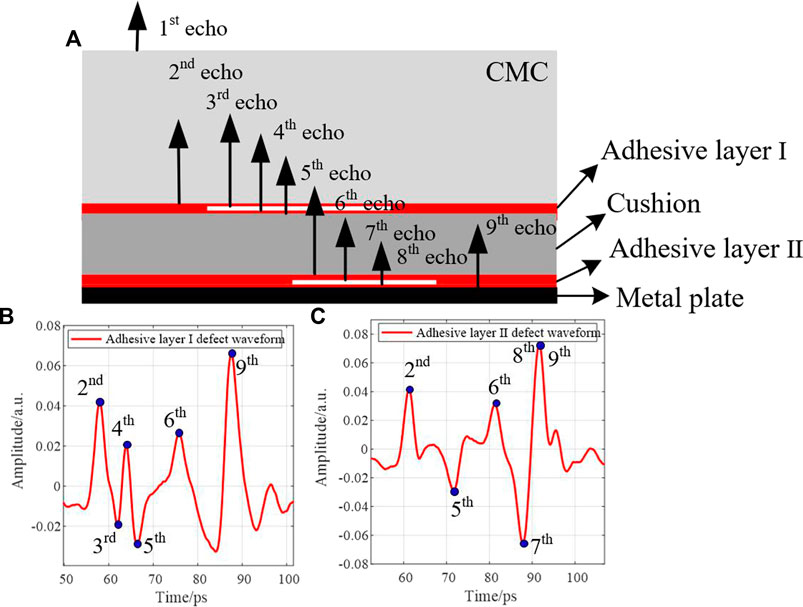
FIGURE 1. Terahertz waveform diagram of the CMC adhesive bonding structure. (A) Schematic diagram of bonding defects, (B) Defect feature waveforms of adhesive layer I, and (C) Defect fea-ture waveforms of adhesive layer II.

In Figure 1, Since the refractive index of CMC is less than that of organosilicon gel, a characteristic peak of second occurs at the interface between CMC and layer I media. The refractive index of organosilicon is greater than that of cushion, forming characteristic Valley fifth at the interface, sixth represents the feature peak at the interface between the cushion and the medium of adhesive layer II, and ninth is the feature peak of the interface reflection between adhesive layer II and the metal plate. Additionally, the THz waveform between the second and ninth refers to the adhesive layer waveform containing the bonding information of the adhesive bonding structure. In this study, only the waveforms in this area are dis-cussed. The THz waveform between the second and fifth represents the waveform in the area of adhesive layer I, and the THz waveform between the sixth and ninth represents the waveform in the area of adhesive layer II.

As shown in Figure 1B, in the presence of a debonding defect in adhesive layer I, the feature peaks third and fourth of the defect were generated during the propagation of the THz waveform in adhesive layer I. When a debonding defect exists in adhesive layer II, the echo valley at the interface between layer II and the metal plate deepens. In addition, the defect features eighth and ninth overlapped because of the existence of side-lobes, scattering, and dispersion. The debonding defects of adhesive layer II were more difficult to recognize than those of adhesive layer I, as demonstrated by the seventh and eighth sections in Figure 1C.

The proportions of THz time-domain sequences of waveform features for different bonding defects are shown in Figure 2, where the dash-and-dot line denotes the defect waveform and the dashed line illustrates the non-defect waveform, the label values in the diagram represent the corresponding horizontal coordinates of the corresponding label points.

FIGURE 2

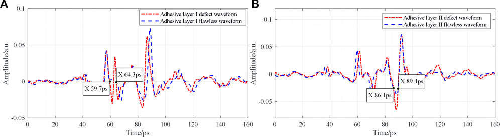
FIGURE 2. Proportions of time-domain sequences of defect features of different adhesive bonding structures: (A) Waveform comparison of adhesive layer I, and (B) Waveform comparison of ad-hesive layer II.

As shown in Figure 2, the defect feature of the waveform of adhesive layer I was 5–6 ps long, and the proportion of the THz waveform of 160 ps was not larger than 3.75%. In contrast, the defect feature of the waveform of adhesive layer II was 3–4 ps long, and the waveform proportion was not larger than 2.5% (Figure 2B). Defect features occupied relatively small proportions in adhesive layers I and II, which is not conducive to defect recognition in the adhesive bonding structure.

4 Methods

4.1 Waveform labeling network

The THz waveforms of the bonding structures under different bonding conditions exhibit different waveform characteristics. The existing THz waveform labeling method involves manually selecting the peaks and valleys of the THz waveform to determine the bonding area. This is time consuming and is highly dependent on the professional knowledge of the operator [27]. Bonding terahertz waveform can predict and label the position of characteristic peaks and valleys from two directions, but using only one direction of time series prediction can not achieve good results. BiLSTM is equivalent to the introduction of “future” data information in the current time period, which is stronger than RNN and LSTM networks in capturing the dependency between time series characteristics [28]. To quickly and accurately label the THz waveforms of bonding structures in different bonding areas, this study constructs a waveform labeling network based on bidirectional LSTM (BiLSTM) and extracts the THz waveforms of different adhesive layers. The BiLSTM network architecture is as shown in Figure 3.

FIGURE 3

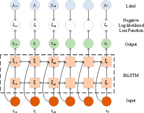
FIGURE 3. BiLSTM network structure.

The operation formula of a memory unit in BiLSTM is as follows:

$\left\{\begin{array}{l}{i}_t=\sigma \left(\left[W_{xi}{W}_{hi}{W}_{ci}1\right]{\left[x_t{h}_{t-1}{c}_{t-1}{b}_i\right]}^T\right)\\ f_t=\sigma \left(\left[W_{xf}{W}_{hf}{W}_{cf}1\right]{\left[x_t{h}_{t-1}{c}_{t-1}{b}_f\right]}^T\right)\\ o_t=\sigma \left(\left[W_{xo}{W}_{ho}{W}_{co}1\right]{\left[x_t{h}_{t-1}{c}_{t-1}{b}_o\right]}^T\right)\\ \stackrel{\sim }{c_t}=\mathit{tanh}\left[W_{xc}{W}_{hc}1\right]{\left[x_t{h}_{t-1}{b}_c\right]}^T\\ c_t=f_t\odot c_{t-1}+i_t\odot \stackrel{\sim }{c_t}\\ h_t=o_t\odot \mathit{tanh}\left(c_t\right)\end{array}\right.(1)$

where $i$, $f$, and $o$ represent the three gates (input gate, forgetting gate, and output gate) activated using the Sigmoid function. $c$ is the unit memory converted by activation. $h_t$ is the output of step $t$ of BiLSTM. $\odot$ represents the element multiplication operation, $W_{jk}$ represents the weight from unit $j$ to unit $k$, $b$ is the offset term, $t$ is the time slot, and $x$ represents the input data. BiLSTM calculates the forward hidden sequence $\overrightarrow{h}$ and backward hidden sequence $\stackrel{⃖}{h}$ in two input directions to obtain the bidirectional information of the time-domain sequence. The calculation formula for the output $z$ is as follows:

$\left\{\begin{array}{l}{\overrightarrow{h}}_t=f\left(\left[W_{x\overrightarrow{h}}{W}_{\overrightarrow{h}\overrightarrow{h}}1\right]{\left[x_t\overrightarrow{h_{t-1}}{b}_{\overrightarrow{h}}\right]}^T\right)\\ {\stackrel{⃖}{h}}_t=f\left(\left[W_{x\overrightarrow{h}}{W}_{\overrightarrow{h}\overrightarrow{h}}1\right]{\left[x_t\stackrel{⃖}{h_{t-1}}{b}_{\stackrel{⃖}{h}}\right]}^T\right)\\ z_t=\left[W_{x\overrightarrow{h}}{W}_{z\stackrel{⃖}{h}}1\right]{\left[\overrightarrow{h_t}\stackrel{⃖}{h_t}{b}_z\right]}^T\end{array}\right.(2)$

To improve the recognition capability of the BiLSTM network, the THz waveform of the bonding structure is first converted into high-level features through a convolution operation and subsequently input into the BiLSTM network layer. The waveform marking network architecture is as shown in Figure 4.

FIGURE 4

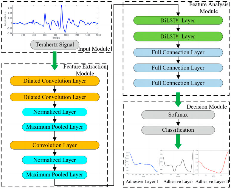
FIGURE 4. Automatic labeling network architecture diagram.

The THz waveform was input into the feature extraction module to extract waveform features, expand the global receptive field through the double-hole convolutional layer, and then the waveform was input into the timing convolutional layer after the normalization operation and maximum pooling to obtain advanced waveform features. The feature analysis module was used to learn the relationship between waveforms in different bonding areas of advanced features, and THz waveform labeling and THz waveform segmentation in different bonding areas were realized through the decision module. The THz data of the same bonding structure sample are marked with a waveform. It took 300 s to manually select the peak and valley of the waveform to determine the bonding area, with an accuracy rate of 98.2%. The marking network took 30 s to do the same task, with an accuracy rate of 97.5%. The results show that the marking accuracy of the marking network and the manual selection method for the THz waveform are similar, but the efficiency is improved by a factor of 10.

4.2 SE attention mechanism

After the extraction of THz waveform features via the neural network, different sampling channels were endowed with the same weight coefficient, which failed to highlight the defect features. In this study, the SE attention mechanism [29, 30] was introduced to accelerate the convergence of the neural network and increase the accuracy of defect recognition. The structure of this mechanism is illustrated in Figure 5.

FIGURE 5

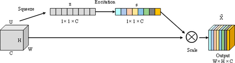
FIGURE 5. Schematic diagram of the SE attention mechanism.

In the traditional SE attention mechanism, the mean value of the feature waveform is taken as the weight distribution index, whereas the weight distribution effect is not evident owing to the randomness of the detection waveforms. Herein, the channel information of the feature waveform was compressed by global variance pooling, and the defect features were assigned a higher weight to improve the feature extraction effect. A comparison of different types of fine granularity waveforms (with 800 data points as examples) is shown in Figure 6, where the dashed and dotted lines represent the defect and non-defect waveforms, respectively.

FIGURE 6

FIGURE 6. Comparison of the defect waveform and non-defect waveform. (A) Fine granularity waveform of adhesive layer I and (B) fine granularity waveform of adhesive layer II.

According to Figure 6A, the defect feature peaks and valleys of the adhesive layer I waveform occurred between data points 237 and 727, whereas the feature waveform experienced oscillation around the zero value. The mean values of the normalized non-defect and defect waveforms were 0.2449 and 0.041, respectively. After global average pooling, the defect feature of the non-defect waveform exhibited a higher weight than that of the defect waveform. Defect features of adhesive layer II were observed between data points 335 and 608, with the mean values of the non-defect and defect waveforms being −0.4305 and −0.1428, respectively (Figure 6B). After the global average pooling of mean values for endowing weights, the weight value of the defect waveform was higher than that of the non-defective waveform; in this case, the output results of the SE module failed to focus completely on the defect features of the waveforms of adhesive layers I and II.

Next, calculation was performed on the global variance pooling of the defect and non-defect waveforms of adhesive layers I and II, with the statistical results shown in Figure 7.

FIGURE 7

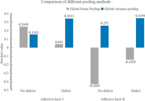
FIGURE 7. Comparison of different pooling methods.

As shown in Figure 7, the defect waveforms of adhesive layers I and II exhibited higher global variance pooling values than the non-defect waveforms, with a larger difference between the defect and non-defective features.

4.3 Multi-feature fusion CNN

The structure of the multi-feature fusion CNN proposed in this study is shown in Figure 8. The THz waveform in the figure was input into the A), B), and C) feature extraction networks, respectively, after the glue layer I waveform, glue layer waveform, and glue layer II waveform were expanded to the same length (the waveform length was unified as 800 data points) after the subsection preprocessing module. The network framework is illustrated in Figure 8.

FIGURE 8

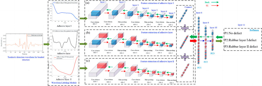
FIGURE 8. Structure diagram of the multi-feature fusion CNN.

For a more comprehensive extraction of waveform features, the sampling group was obtained by adding three groups of convolutional layers and the maximum pooling layer to the first convolutional layer, which was subsequently used to extract the waveform features output by the up-sampling layer. During the feature extraction, the feature weights were adjusted using the SE attention mechanism. According to the amount of defect feature in-formation, the waveform features extracted by the last maximum pooling layer were endowed with different weights and sequentially connected. The defect feature information was statistically analyzed based on three fully connected layers. Finally, the waveform type probability was output using the softmax function. The network parameters are listed in Table 1.

TABLE 1

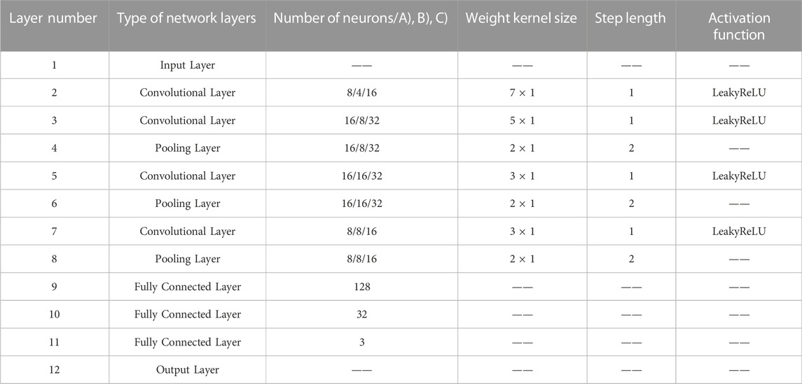
TABLE 1. Network parameters.

The learning speed of the traditional rectified linear unit (ReLU) can decrease or even become zero when the input features have negative values. Since the input is lesser than zero and the gradient is equal to zero, the network weights cannot be updated and remain constant throughout the rest of the time. To avoid the “dead neuron” phenomenon, the traditional ReLU function was replaced with the LeakyReLU function [31] in this study. As a variant of the ReLU function, the latter assigns non-zero outputs to negative input in-formation, as expressed in Eq. 3:

$f\left(x\right)=\mathit{max}\left(\alpha x,x\right)(3)$

where $\alpha$ denotes a predefined parameter within (0, 1), and $x\in R$. Unlike ReLU, which maps negative input information to zero, LeakyReLU compresses negative input information with a predefined linear function, maintaining the negative part of feature information and weighing network scarcity and input information.

5 Sample design

To build a neural network database and prepare samples with various bonding defects, polytetrafluoroethylene (PTFE) defect sample sheets with a diameter of 20 mm and varying thicknesses were pre-embedded in the upper and lower adhesive layers of the edge area of the sample [3] (Figure 9A). After complete curing of the organic glue, the defect sample sheets were withdrawn to form air gaps between the adhesive layers to simulate debonding defects of different thicknesses in varying adhesive layers. The design diagram and number of pre-embedded defects are shown in Figures 9A, B, respectively.

FIGURE 9

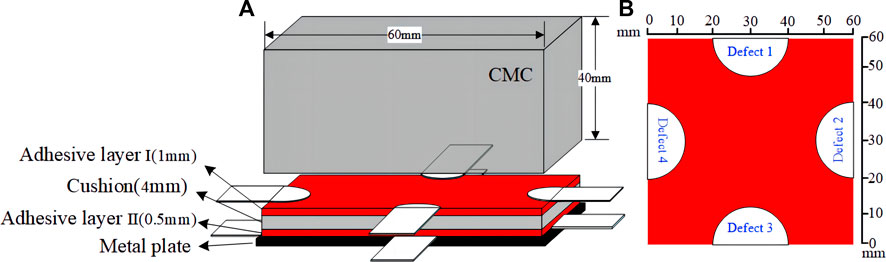
FIGURE 9. Sample design.

Adhesive bonding structure samples were prepared in accordance with the sample design diagram given in Figure 9, with the types of debonding samples listed in Table 2. One of the samples with different debonding thicknesses was extracted to conduct the network generalization test, and the remaining samples were applied to the construction of the network dataset.

TABLE 2

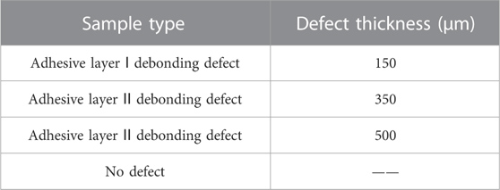
TABLE 2. Network parameters.

6 Results and discussion

6.1 Data set description

The THz waveforms of different debonding defect types were obtained from the defect and non-defect areas of the adhesive bonding structure samples, forming the dataset “Data for Terahertz” for defect recognition of the adhesive bonding structure (Table 3).

TABLE 3

TABLE 3. Composition of the dataset.

6.2 Influence of waveform labeling preprocessing module on the performance of the proposed network

Considering the influence of the waveform marking preprocessing module on the recognition effect of the multi-feature fusion CNN, and comparing the recognition effect of the network proposed in this study to determine whether the input waveform passed through the waveform marking preprocessing module, Figures 10A, B, respectively, show the recognition accuracy curve of the network in this study and the iterative loss curve of defect recognition training when the input waveform has passed the waveform marking preprocessing. The dashed line in the figure represents the network recognition result of the input data without the waveform marking preprocessing module, and the dotted line is the network recognition result of the input data after the waveform marking preprocessing module.

FIGURE 10

FIGURE 10. Comparison of the network performance under different inputs: (A) accuracy curve and (B) loss function curve. Schematic diagram of the interference signal generated by the metal plate.

It can be observed from the curve in Figure 10A that when the dataset is directly used as the network input, the accuracy curve is always below the identification accuracy curve with the waveform of the waveform marking preprocessing module as the network input, and the final accuracies are 98.13% and 99.28%, respectively. When the defect features occupy a small proportion in the input waveform, it is easily submerged in the process of feature extraction of the CNN network, and the feature extraction results of different CNN networks on the input waveform are different. After the channel weights are provided and connected by the SE attention mechanism, the final defect feature statistics may change unpredictably, resulting in the incomplete extraction of defect feature information from the network. This may affect the accuracy of network identification. As shown in Figure 10B, after the input waveform passed through the waveform marking preprocessing module, the loss function of the network decreased faster, and the final network losses caused by the input waveforms with different granularities were 0.032 and 0.013, respectively. Hence, the following conclusions can be drawn from the above: the network has a greater response to the input of the fine-grained waveform, the characteristic defects account for a large proportion of the input waveform, the defect feature information extracted from different CNNs is more complete, and the model recognition accuracy is higher.

6.3 Performance comparison of different networks

The performance of the constructed defect-recognition network and other defect-recognition methods was compared in terms of accuracy (ACC), sensitivity, precision, and comprehensive evaluation index F1. To validate the advantages of the constructed network, the recognition results of different classification methods on the dataset “Data for Terahertz” were compared, as shown in Table 4. The highest recognition result of different algorithms is shown in bold in the table.

TABLE 4

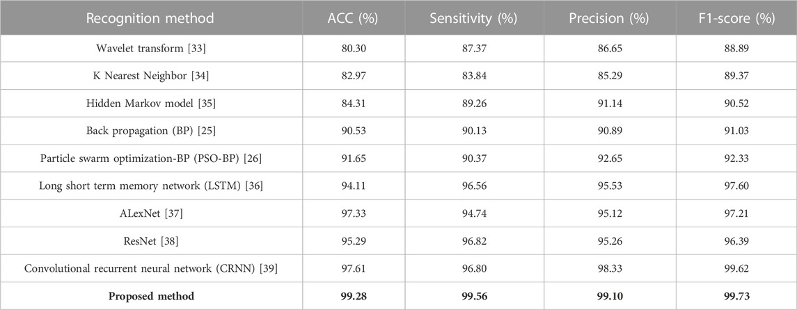
TABLE 4. Classification results of different methods.

As shown in Table 4, the recognition accuracy of the wavelet transform, K nearest neighbor, and hidden Markov model for the THz waveforms of the adhesive bonding structure were 80.30%, 82.97%, and 84.3%, respectively, with low precision of target feature recognition. The recognition accuracy of BP neural network and PSO-BP neural network is 90.53% and 91.65% respectively. Because the input of BP and PSO-BP network is waveform feature, the network lacks the tiny feature information of waveform, which affects the recognition result of the network; LSTM recognizes the relationship between waveform features through long-term and short-term memory units, and the final recognition accuracy is 94.11%, sensitivity is 96.56%, accuracy is 95.53%, and F1 score is 97.60%. ALexNet and ResNet extract and transmit waveform features through neurons. After multiple network layers such as convolution, pooling, and full connection, the relatively small defect features are easy to be submerged, resulting in the network’s final recognition accuracy of 97.33% and 95.29%, sensitivity of 94.74% and 96.82%, accuracy of 95.12% and 95.26%, and F1 scores of 97.21% and 96.39%; CRNN network extracts waveform features through convolutional layer and pooling layer, and uses RNN network layer to analyze the relationship between features. The final recognition accuracy is 97.61%, sensitivity is 96.80%, accuracy is 98.33%, and F1 score is 99.62%. In this paper, the network recognition accuracy rate is 99.28%, sensitivity is 99.56%, accuracy is 99.10%, F1 score is 99.73%, and the performance on the data set is the best. The multi feature fusion model built in literature [32] has a low recognition accuracy in image classification, mainly because the traditional SE attention mechanism added after image feature extraction in document [32] does not suppress useless features during feature extraction, but the network model built in this paper adds an improved SE attention mechanism after each sampling layer to suppress useless features, accelerate network convergence and improve recognition effect. So the network built in document [32] has less influence on data feature selection than the network model built in this paper. The statistics of the iteration losses in defect recognition training using different networks and partial network confusion matrices were obtained, as shown in Figure 11 and Figure 12, respectively.

FIGURE 11

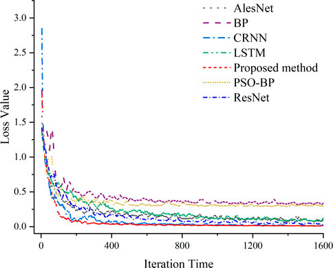
FIGURE 11. Iteration loss curves in the defect recognition training by different networks.

FIGURE 12

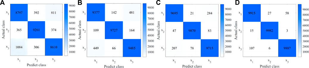
FIGURE 12. Partial network confusion matrices. (A) BP, (B) ResNet, (C) CRNN, and (D) Proposed method.

The loss curves of 1,600 defect-recognition iterations for different networks are plotted in Figure 11. The loss curve of the proposed method was below that of all other networks, yielding a loss value of 0.013, followed by CRNN with a loss value of 0.02. The loss curves of BP and PSO-BP neural networks exhibited the lowest decrease speed and became stable at 1,000 iterations with loss values of 0.34 and 0.30, respectively. The loss values of ResNet network, LSTM network and ALexNet network are 0.05, 0.09 and 0.10 respectively.

In Figure 12, x₁, x₂, and x₃ denote the non-defect waveform, defect waveform of adhesive layer I, and defect waveform of adhesive layer II, respectively. As can be seen in the figure, the BP neural network could determine a total of 811 defect waveforms of adhesive layer II in 10,000 non-defect waveforms and 1,084 non-defective waveforms in 10,000 defect waveforms of adhesive layer II, indicating that the BP neural network was prone to defect feature confusion, showing poor defect recognition accuracy. In contrast, ResNet and CRNN exhibited a recognition accuracy of over 93% and a better recognition effect in the defect waveforms of adhesive layer I than those of adhesive layer II. The defect features of adhesive layer II, which were similar to those of the non-defect waveforms, were sub-merged in the feature extraction process, resulting in incomplete statistical defect features of the fully connected layer. This caused confusion in the classification results of the non-defect and defect waveforms. The proposed method achieved accuracies of 99.15%, 99.82%, and 98.87% in recognition of the defect waveforms of adhesive layer I, adhesive layer II, and non-defect waveforms, respectively, indicating the best recognition effect on the bonding defects of different adhesive bonding structures. Thus, the proposed method could fully recognize the defect waveform features of adhesive layer II and non-defect waveform features, and reduce the network recognition error rate.

6.4 Defect recognition results

The key to network performance testing is accurate recognition of waveforms at the junction between the defect and normal areas. The defect waveforms in the edge areas were similar to those in the non-defective areas. The comparison of feature waveforms between different adhesive bonding areas of the 150 µm pre-embedded defect samples of adhesive layer I and those of the 350 µm pre-embedded defect samples of adhesive layer II are shown in Figure 13A, B, respectively. The dash-dot, dashed, and dotted lines represent the waveforms in the defect, edge, and non-defect areas, respectively.

FIGURE 13

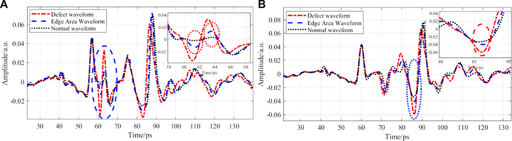
FIGURE 13. Comparison of adhesive layer waveforms in different areas (A) Comparison of feature waveforms of adhesive layer I and (B) adhesive layer II.

In Figure 13A, more prominent waveform features can be observed in the defect area of adhesive layer I. In the waveform area of adhesive layer I, oscillating peaks and valleys were generated by the reflected echoes at the THz interface between the organic glue and air gap. Similar waveform features in the edge and non-defect areas can be observed in the amplitude of the peak-to-valley oscillation in the red circle area in Figure 13A. Hence, the waveform features in the edge area were easily submerged in the waveform feature extraction of the non-defect area, resulting in network confusion regarding the analysis and statistics of the waveform information in the defect, edge, and non-defect areas. This eventually influences the waveform recognition accuracy in different areas. According to the waveforms in the defect area of adhesive layer II (Figure 13B), the difference between waveforms in these three areas was only represented by the size of the valley in the red circle area owing to the superposition of the side lobe information of THz signals. This makes it difficult for the network to accurately recognize the waveforms in the defect and defect edge areas during the extraction of waveform features, resulting in recognition errors.

The proposed network after training, the BP neural network in the literature [25], and the CRNN with the best performance in the classification results were used to recognize the generalized samples with different debonding thicknesses, as shown in Figure 14. The first, second, and third rows denote the recognition results of the 150 µm pre-embedded defect sample of adhesive layer I, the 350 µm pre-embedded defect sample of adhesive layer II, and the 500 µm pre-embedded defect sample of adhesive layer II, respectively. The bonding defect areas recognized by the network model and the non-defect areas are marked in red and blue, respectively. The closer the chromaticity is to red, the larger is the defect probability. To quantify the recognition ability of different networks for pre-embedded defects, the statistical results of networks, i.e., the proportion Nor-Def of the number of non-defective waveforms, erroneously determined as defective waveforms in the overall number of non-defective waveforms, and the proportion Def-Nor of the number of defective waveforms, erroneously determined as non-defective waveforms in the overall number of defective waveforms, were obtained, as listed in Table 5.

FIGURE 14

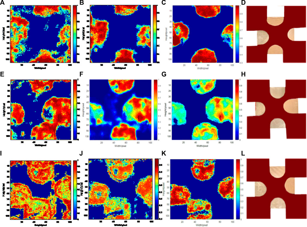
FIGURE 14. Recognition results of different pre-embedded defect samples by different networks: (A) the BP neural network for the 150 μm defect sample of adhesive layer I, (B) the CRNN for the 150 μm defect sample of adhesive layer I, (C) the proposed method for the 150 μm defect sample of adhesive layer I, and (D) the actual 150 μm pre-embedded defect sample of adhesive layer I. (E) Recognition results of the BPNN for the 350 μm defect sample of adhesive layer II, (F) the CRNN for the 350 μm defect sample of adhesive layer II, (G) the proposed method for the 350 μm defect sample of adhesive layer II, (H) and the actual 350 μm pre-embedded defect sample of adhesive layer II. (I) Recognition results of the BP neural network for the 500 μm de-fect sample of adhesive layer II, (J) the CRNN for the 500 μm defect sample of adhesive layer II, (K) the proposed method for the 500 μm defect sample of adhesive layer II, and (L) the actual 500 μm pre-embedded defect sample of adhesive layer II.

TABLE 5

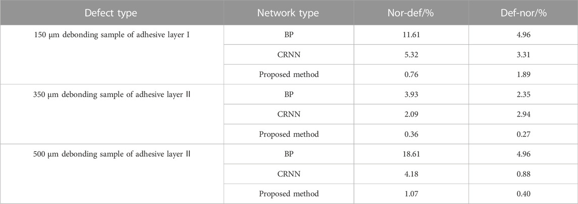
TABLE 5. Statistics of the defect recognition error rates of different networks.

The recognition results of the different networks regarding the pre-embedded defect samples are shown in Figure 14. According to the recognition results of the BP, CRNN, and proposed method for 150 μm pre-embedded defect samples of adhesive layer I shown in Figures 14A–C, the defect location recognized by the BP neural network was not consistent with the location of the pre-embedded defect, and the defect area surrounded the pre-embedded defect. Moreover, the BP neural network confused part of the non-defect waveform with the defect waveform of the adhesive layer I. The determined ratios of the defect areas of defects 1, 2, 3, and 4 to the pre-embedded defect area in the recognition results of this network were 112.35%, 104.83%, 95.11%, and 121.25%, respectively, showing large differences between the recognition results and the theoretical area. In addition, the network exhibited high Nor-Def and Def-Nor values and a poor waveform recognition of the defect edge area. The CRNN accurately recognized the location of the pre-embedded defect, with no stray defect area surrounding it. However, it recognized part of the defect waveform of adhesive layer I as a non-defective waveform, obtained a Def-Nor value of 3.31% and a Nor-Def value of 5.32%, and displayed a low accuracy in recognizing the waveform in the defect edge area. The defect recognition results of the proposed network are given in Figure 14C, showing the basic consistency between the location of the recognized defect and the defect area of the pre-embedded sample. The ratios of the defect recognition areas of defect 1, 3, and 4 to the theoretical pre-embedded defect area were all greater than 96%, together with a Nor-Def value of 0.76% and a Def-Nor value of 1.89%. The proposed network exhibited a good waveform recognition effect in the transition area, with the shape of the recognized defect being consistent with that of the pre-embedded defect. The difference between the defect recognition area of Defect 2 and the pre-embedded defect area can be observed in Figure 14C because problems in the production process can lead to a blurred interface between the defective and normal areas in some areas, resulting in an inconsistency between the final recognition result and the oretical area.

According to the recognition results for the 350 µm pre-embedded defect sample of adhesive layer II (Figure 14E–G), the location of the pre-embedded defect was recognized by all three defect recognition networks. However, the BP neural network obtained a Def-Nor value of 2.35%, which was concentrated around defect 2. It also displayed a weak resistance to random errors in sample production and confused the defect waveforms and normal area waveforms, eventually generating a stray defect area in the defect recognition result map. The CRNN accurately recognized the defect location, but showed low precision in recognizing the waveform of the defect edge area, obtaining Nor-Def and Def-Nor values of 2.09% and 2.94%, respectively. In the network recognition results of the pro-posed network, no stray defect areas existed around the pre-embedded defect, with Nor-Def and Def-Nor values of 0.36% and 0.27%, respectively. Moreover, the proposed network could correctly discrimination between different types of waveforms and showed a low defect recognition error rate.

The recognition results of the 500 µm pre-embedded defect sample of adhesive layer II are plotted in Figures 14I–K. It can be observed from the combination of Figure 14 and Table 5 that the proposed network has the lowest Nor-Def and Def-Nor values (1.07% and 0.40%, respectively), high waveform recognition accuracy, and better recognition results than those of the BP neural network and CRNN. Moreover, it could differentiate between the defect waveform and the normal area waveform, resulting from uncertain factors during sample production. The ratios of the defect areas of defects 1, 2, 3, and 4 to the pre-embedded defect area in the recognition results of this network were 93.73%, 98.16%, 93.36%, and 95.55%, respectively. A relatively high consistency was obtained between the recognized defect location and area and that of the pre-embedded defect.

According to the recognition results of the three networks in terms of the pre-embedded defect samples, the existing methods for defect recognition of adhesive bonding structures only improve the feature recognition accuracy by means of prepro-cessing detection waveforms or adjusting algorithm parameters but fail to improve it from the perspective of the essence of target feature recognition. Herein, the single detection waveform was segmented by the adhesive bonding area, and the waveforms in different adhesive bonding areas were input as a multichannel CNN after the subtraction operation to increase the proportion of waveform features. Moreover, the SE attention mechanism was used to increase the weight of defect features. The proposed network obtained higher values of all these indices, including the ratio of the recognized defect area to the pre-embedded defect area, the waveform recognition accuracy of the defect edge area, and the Nor-Def and Def-Nor values in the defect recognition of generalized samples, com-pared to the BP neural network and the CRNN, demonstrating its advantages in defect recognition of adhesive bonding structures.

7 Conclusion

In this study, according to the interface characteristics of the bonding-structure THz-detection waveform, a multi-feature fusion convolutional neural network was constructed for bonding quality detection of bonded structures. After the preprocessing of waveform marking as the network input, with the segmented waveforms of different bonding areas, the channel weights were allocated through the SE attention mechanism. The feature extraction results of multiple neural networks were integrated and the classified detection waveforms were identified. The comparison results of different granularity waveform inputs of the network in this study show that a fine granularity waveform of the bonding area can better simulate the feature extraction ability of the network and improve its recognition and classification effect. The results show that the efficiency of the labeling network is 10 times higher than that of manual selection. The accuracy of the defect recognition network in this study was 99.28%, sensitivity was 99.56%, accuracy was 99.10%, and F1 score was 99.73%, which was the best in the dataset. Compared with the BP and CRNN networks, the labeling network performed better in the preset defect detection of generalized experimental samples; the lowest obtained error rate of defect recognition was 0.27%. The proposed network solves the problems of low efficiency of the defect identification method of adhesive structures and considerable influence of subjective factors, and promotes the development of THz non-destructive testing technology. We would like to thank Editage (www.editage.cn) for English language editing.

Data availability statement

The data presented in this study are available on request from the corresponding author.

Author contributions

For research articles with several authors, a short paragraph specifying their individual contributions must be provided. The following statements should be used “Conceptualization, WX; methodology, WX; software, QC; validation, JR, DZ, and JG; formal analysis, LL; investigation, WX; resources, WX; data curation, WX; writing—original draft preparation, WX; writing—review and editing, WX; visualization, WX; supervision, JX; project administration, WX; funding acquisition, JZ. All authors have read and agreed to the published version of the manuscript”.

Funding

This research was supported by the Jilin Province science and technology development plan project with grant No. 20220508032RC, as well as the second batch of social welfare and basic research projects in Zhongshan with grant No. 2022B2012. We would like to thank Changchun University of Science and Technology for the use of their equipment.

Conflict of interest

The authors declare that the research was conducted in the absence of any commercial or financial relationships that could be construed as a potential conflict of interest.

Publisher’s note

All claims expressed in this article are solely those of the authors and do not necessarily represent those of their affiliated organizations, or those of the publisher, the editors and the reviewers. Any product that may be evaluated in this article, or claim that may be made by its manufacturer, is not guaranteed or endorsed by the publisher.

References

1. Pisharody AP, Smith DE. Effect of interlayer adherend inclusions on strength of composite bonded joints. Compos Structures (2022) 291:115531. doi:10.1016/j.compstruct.2022.115531

CrossRef Full Text | Google Scholar

2. Saeedifar M, Zarouchas D. Damage characterization of laminated composites using acoustic emission: A review. Composites B: Eng (2020) 195:108039. doi:10.1016/j.compositesb.2020.108039

CrossRef Full Text | Google Scholar

3. Wang Q, Li X, Chang T, Zhang J, Liu L, Zhou H, et al. Nondestructive imaging of hidden defects in aircraft sandwich composites using terahertz time-domain spectroscopy. Infrared Phys Tech (2019) 97:326–40. doi:10.1016/j.infrared.2019.01.013

CrossRef Full Text | Google Scholar

4. Garnier C, Pastor ML, Eyma F, Lorrain B. The detection of aeronautical defects in situ on composite structures using Non Destructive Testing. Compos structures (2011) 93(5):1328–36. doi:10.1016/j.compstruct.2010.10.017

CrossRef Full Text | Google Scholar

5. Sun J, Ye D, Zou J, Chen X, Wang Y, Yuan J, et al. A review on additive manufacturing of ceramic matrix composites. J Mater Sci Tech (2022) 138:1–16. doi:10.1016/j.jmst.2022.06.039

CrossRef Full Text | Google Scholar

6. Rahani EK, Kundu T, Wu Z, Xin H. Mechanical damage detection in polymer tiles by THz radiation. IEEE Sensors J (2010) 11(8):1720–5. doi:10.1109/jsen.2010.2095457

CrossRef Full Text | Google Scholar

7. Shen X, Dietlein CR, Grossman E, Popovic Z, Meyer FG. Detection and segmentation of concealed objects in terahertz images. IEEE Trans Image Process (2008) 17(12):2465–75. doi:10.1109/tip.2008.2006662

PubMed Abstract | CrossRef Full Text | Google Scholar

8. Fuse N, Fukuchi T, Takahashi T, Mizuno M, Fukunaga K. Evaluation of applicability of noncontact analysis methods to detect rust regions in coated steel plates. IEEE Trans Terahertz Sci Tech (2012) 2(2):242–9. doi:10.1109/tthz.2011.2178932

CrossRef Full Text | Google Scholar

9. Zhang JY, Ren JJ, Li LJ, Gu J, Zhang DD. THz imaging technique for nondestructive analysis of debonding defects in ceramic matrix composites based on multiple echoes and feature fusion. Opt express (2020) 28(14):19901–15. doi:10.1364/oe.394177

PubMed Abstract | CrossRef Full Text | Google Scholar

10. Wu D, Haude C, Burger R, Peters O. Application of terahertz time domain spectroscopy for NDT of oxide-oxide ceramic matrix composites. Infrared Phys Tech (2019) 102:102995. doi:10.1016/j.infrared.2019.102995

CrossRef Full Text | Google Scholar

11. Zhang DD, Ren JJ, Gu J, Li LJ, Zhang JY, Xiong WH, et al. Nondestructive testing of bonding defects in multilayered ceramic matrix composites using THz time domain spectroscopy and imaging. Compos Structures (2020) 251:112624. doi:10.1016/j.compstruct.2020.112624

CrossRef Full Text | Google Scholar

12. Ruhunusiri S. Identification of plasma waves at saturn using convolutional neural networks. IEEE Trans Plasma Sci (2018) 46(8):3090–9. doi:10.1109/tps.2018.2849940

PubMed Abstract | CrossRef Full Text | Google Scholar

13. Li Y, Xue D, Forrister E, Lee G, Garner B, Kim Y. Human activity classification based on dynamic time warping of an on-body creeping wave signal. IEEE Trans Antennas Propagation (2016) 64(11):4901–5. doi:10.1109/tap.2016.2598199

CrossRef Full Text | Google Scholar

14. Cheng X, Li G, Ellefsen AL, Chen S, Hildre HP, Zhang H. A novel densely connected convolutional neural network for sea-state estimation using ship motion data. IEEE Trans Instrumentation Meas (2020) 69(9):5984–93. doi:10.1109/tim.2020.2967115

CrossRef Full Text | Google Scholar

15. Lian F, Xu D, Fu M, Ge H, Jiang Y, Zhang Y. Identification of transgenic ingredients in maize using terahertz spectra. IEEE Trans Terahertz Sci Tech (2017) 7(4):378–84. doi:10.1109/tthz.2017.2708983

CrossRef Full Text | Google Scholar

16. Dorney TD, Baraniuk RG, Mittleman DM. Material parameter estimation with terahertz time-domain spectroscopy. JOSA A (2001) 18(7):1562–71. doi:10.1364/josaa.18.001562

PubMed Abstract | CrossRef Full Text | Google Scholar

17. Zhou Y, Xu J, Liu Q, Li C, Liu Z, Wang M, et al. A radiomics approach with CNN for shear-wave elastography breast tumor classification. IEEE Trans Biomed Eng (2018) 65(9):1935–42. doi:10.1109/tbme.2018.2844188

PubMed Abstract | CrossRef Full Text | Google Scholar

18. Sun F, Fan M, Cao B, Zheng D, Liu H, Liu L. Terahertz based thickness measurement of thermal barrier coatings using long short-term memory networks and local extrema. IEEE Trans Ind Inform (2021) 18(4):2508–17. doi:10.1109/tii.2021.3098791

CrossRef Full Text | Google Scholar

19. Cruz FC, Simas Filho EF, Albuquerque MCS, Silva IC, Farias CTT, Gouvêa LL. Efficient feature selection for neural network based detection of flaws in steel welded joints using ultrasound testing. Ultrasonics (2017) 73:1–8. doi:10.1016/j.ultras.2016.08.017

PubMed Abstract | CrossRef Full Text | Google Scholar

20. Meng M, Chua YJ, Wouterson E, Ong CPK. Ultrasonic signal classification and imaging system for composite materials via deep convolutional neural networks. Neurocomputing (2017) 257:128–35. doi:10.1016/j.neucom.2016.11.066

CrossRef Full Text | Google Scholar

21. Hu C, Duan Y, Liu S, Yan Y, Tao N, Osman A, et al. LSTM-RNN-based defect classification in honeycomb structures using infrared thermography. Infrared Phys Tech (2019) 102:103032. doi:10.1016/j.infrared.2019.103032

CrossRef Full Text | Google Scholar

22. Wang Q, Liu Q, Xia R, Zhang P, Zhou H, Zhao B, et al. Automatic defect prediction in glass fiber reinforced polymer based on THz-TDS signal analysis with neural networks. Infrared Phys Tech (2021) 115:103673. doi:10.1016/j.infrared.2021.103673

CrossRef Full Text | Google Scholar

23. Xu Y, Zhou H, Cui Y, Wang X, Citrin DS, Zhang L, et al. Full scale promoted convolution neural network for intelligent terahertz 3D characterization of GFRP delamination. Composites Part B: Eng (2022) 242:110022. doi:10.1016/j.compositesb.2022.110022

CrossRef Full Text | Google Scholar

24. Liu W, Wang Q, Zhang H, Li Z, Liu Q, She R, Zhang R. Automatic terahertz recognition of hidden defects in layered polymer composites based on a deep residual network with transfer learning. In: Proceeding of the 2021 46th International Conference on Infrared, Millimeter and Terahertz Waves (IRMMW-THz); October 2021Chengdu, China. IEEE (2021). p. 1.

CrossRef Full Text | Google Scholar

25. Ren J, Li L, Zhang D, Qiao X, Lv Q, Cao G. Study on intelligent recognition detection technology of debond defects for ceramic matrix composites based on terahertz time domain spectroscopy. Appl Opt (2016) 55(26):7204–11. doi:10.1364/ao.55.007204

PubMed Abstract | CrossRef Full Text | Google Scholar

26. Jia MH, Li LJ, Ren JJ. Terahertz nondestructive testing signal recognition based on PSO-BP neural network. Acta PhotonicaSinica (2021) 50(0930004):10–3788. doi:10.3788/gzxb20215009.0930004

CrossRef Full Text | Google Scholar

27. Wang Q, Zhou H, Xia R, Liu Q, Zhao BY. Time segmented image fusion based multi-depth defects imaging method in composites with pulsed terahertz. IEEE Access (2020) 8:155529–37. doi:10.1109/access.2020.3019319

CrossRef Full Text | Google Scholar

28. Yildirim Ö. A novel wavelet sequence based on deep bidirectional LSTM network model for ECG signal classification. Comput Biol Med (2018) 96:189–202. doi:10.1016/j.compbiomed.2018.03.016

PubMed Abstract | CrossRef Full Text | Google Scholar

29. Naranjo-Alcazar J, Perez-Castanos S, Zuccarello P, Cobos M. Acoustic scene classification with squeeze-excitation residual networks. IEEE Access (2020) 8:112287–96. doi:10.1109/access.2020.3002761

CrossRef Full Text | Google Scholar

30. Jia N, Tian X, Zhang Y, Wang F. Semi-supervised node classification with discriminable squeeze excitation graph convolutional networks. IEEE Access (2020) 8:148226–36. doi:10.1109/access.2020.3015838

CrossRef Full Text | Google Scholar

31. Xu B, Wang N, Chen T, Li M. Empirical evaluation of rectified activations in convolutional network (2015). arXiv preprint arXiv:1505.00853.

Google Scholar

32. Liu J, Zhang J. Dssemff: A depthwise separable squeeze and excitation based on multi-feature fusion for image classification. Sensing and Imaging (2022) 23(1):16–8. doi:10.1007/s11220-022-00383-5

CrossRef Full Text | Google Scholar

33. Ho KC, Prokopiw W, Chan YT. Modulation identification of digital signals by the wavelet transform[J]. IEE Proceedings-Radar, Sonar and Navigation (2000) 147(4):169–176.

CrossRef Full Text | Google Scholar

34. Chen CH, Huang WT, Tan TH, Chang CC, Chang YJ. Using k-nearest neighbor classification to diagnose abnormal lung sounds. Sensors (2015) 15(6):13132–58. doi:10.3390/s150613132

PubMed Abstract | CrossRef Full Text | Google Scholar

35. Bozkurt B, Germanakis I, Stylianou Y. A study of time-frequency features for CNN-based automatic heart sound classification for pathology detection. Comput Biol Med (2018) 100:132–43. doi:10.1016/j.compbiomed.2018.06.026

PubMed Abstract | CrossRef Full Text | Google Scholar

36. Cai W, Zhang W, Hu X, Liu Y. A hybrid information model based on long short-term memory network for tool condition monitoring. J Intell Manufacturing (2020) 31(6):1497–510. doi:10.1007/s10845-019-01526-4

CrossRef Full Text | Google Scholar

37. Ismail Fawaz H, Lucas B, Forestier G, Pelletier C, Schmidt DF, Weber J, et al. Inceptiontime: Finding alexnet for time series classification. Data Mining Knowledge Discov (2020) 34(6):1936–62. doi:10.1007/s10618-020-00710-y

CrossRef Full Text | Google Scholar

38. Zhang Y, Li J, Wei S, Zhou F, Li D. Heartbeats classification using hybrid time-frequency analysis and transfer learning based on ResNet. IEEE J Biomed Health Inform (2021) 25(11):4175–84. doi:10.1109/jbhi.2021.3085318

PubMed Abstract | CrossRef Full Text | Google Scholar

39. Cakır E, Parascandolo G, Heittola T, Huttunen H, Virtanen T. Convolutional recurrent neural networks for polyphonic sound event detection. IEEE/ACM Trans Audio, Speech, Lang Process (2017) 25(6):1291–303. doi:10.1109/taslp.2017.2690575

CrossRef Full Text | Google Scholar