Rich dynamics of a vegetation–water system with the hydrotropism effect

In recent years, with the abnormal global climate change, the problem of desertification has become more and more serious. The vegetation pattern is accompanied by desertification, and thus, the study of the vegetation pattern is helpful to better understand the causes of desertification. In this work, we reveal the influences of hydrotropism on the vegetation pattern based on a vegetation–water system in the form of reaction–diffusion equations. Parameter ranges for the steady-state mode obtained by analyzing the system show the dynamic behavior near the bifurcation point. Furthermore, we found that vegetation hydrotropism not only induces spatial pattern generation but also promotes the growth of vegetation itself in this area. Therefore, through the study of vegetation patterns, we can take corresponding preventive measures to effectively prevent land desertification and improve the stability of the ecosystem in the region.

1 Introduction

Vegetation is an important part of nature and plays a leading role in the ecosystem, known as the “Ecological Engineer” [1, 2]. As a producer, vegetation can convert carbon dioxide into carbohydrates through photosynthesis and release oxygen and store energy. Moreover, vegetation coverage on the ground can not only reduce water and soil loss and protect slope land but also prevent wind and sand fixation and prevent desertification [3, 4]. In nature, the growth of vegetation will be affected by climatic conditions, geographical environment, and human activities. Nowadays, with the rapid development of irrationality in the human society and global climate change, the vegetation ecosystem has been seriously damaged, and the problem of land desertification is becoming more and more serious [5–7].

In particular, in dry and semi-dry areas, because of its climatic characteristics, the problem of land desertification is particularly prominent. In the process of land desertification, vegetation distribution is uneven, but there are certain rules. We call this uneven and regular spatial distribution of vegetation as the vegetation pattern [8–10]. In addition, different vegetation pattern structures have different significances to the function of the ecosystem, such as the strip pattern can be used as a sign of semi-desert [11]. For the study of vegetation spatial patterns in these areas, many scholars established a series of a dynamic system. Based on ecologically realistic assumptions, Klausmeier established a model with vegetation and water in 1999 and gave suitable parameters, and two pattern types can be found by numerical simulations (regular patterns and irregular patterns). This model helps us understand how rainfall and grazing affect vegetation in semi-arid regions and demonstrates the importance of non-linear mechanisms to the spatial structure of plant community [12]. In 2001, Von Hardenberg proposed a new vegetation–water system, which simulates the competition of vegetation roots for water resources [13]. In 2007, Gilad constructed a mathematical system for the study of the woody plant ecosystem in arid areas and captured various feedback mechanisms between biomass and water resources through this system [14]. Water diffuses freely in soil, and the original Klausmeier system does not consider the diffusion of water. Therefore, Vander Stelt took the diffusion of water into account on the basis of Klausmeier’s system in 2012 [15]. In 2015, Zelnik simplified Gilad’s model and combined with empirical data to study the dynamics of Namibia’s Andromeda ecosystem. The research showed that the pattern trend changes gradually in the spatially expanded ecosystem [16]. Moreover, other scholars have also established relevant systems to study vegetation patterns [17–25].

It is known to all that water is the source of life. Vegetation needs water for photosynthesis and respiration to obtain nutrients needed for vegetation growth. Moreover, when transpiration takes away a lot of heat, water can maintain the normal temperature of vegetation to maintain life activities [26, 27]. Vegetation absorbs water from the soil mainly through the root system to provide water necessary for life activities. In response to a moisture gradient, the roots of vegetation will show the characteristics of hydrotropism [28–31]. In dry and semi-dry areas, soil water distribution is uneven because of less and concentrated rainfall [32, 33]. Therefore, the vegetation root system will absorb the water in other humid areas through the extension of the root system to meet its own growth and development in these areas. At present, it is not clear how the hydrotropism effect of vegetation roots affects the growth and distribution of vegetation. Therefore, to reveal the influence of hydrotropism of vegetation roots on vegetation growth and distribution, we build a spatial system with root hydrotropism effects based on the system of Klausmeier in this paper [34–36].

The following is the content arrangement of this article. In the first place, we propose a reaction–diffusion system with hydrotropism effects and analyze the existence and stability about the equilibrium point. In the next section, we derive the amplitude equation and its coefficients through the method of multi-scale analysis. In the fourth section, on the basis of the theoretical results obtained in the previous section, we conduct a numerical simulation to obtain the dynamic behavior and show the hydrotropism of vegetation’s impact on the vegetation pattern. Finally, the last section gives conclusions and discussions on the effect of hydrotropism on vegetation growth and distribution.

2 Mathematical model and analysis

2.1 Mathematical model

In dry and semi-dry regions, soil water replenishment was mainly derived from rainfall due to their geographical environment. After the rainfall reaches the ground, one part of the rainfall penetrates into the soil and becomes groundwater or surface runoff, and the other part is lost to the atmosphere through the transpiration of vegetation and evaporation of the ground. These areas receive less rainfall because of their climatic conditions. Therefore, soil water distribution in these areas is uneven, forming a moisture gradient. In response to a moisture gradient, the roots of vegetation will show the characteristics of hydrotropism to get more water for basic life activities (Figure 1).

FIGURE 1

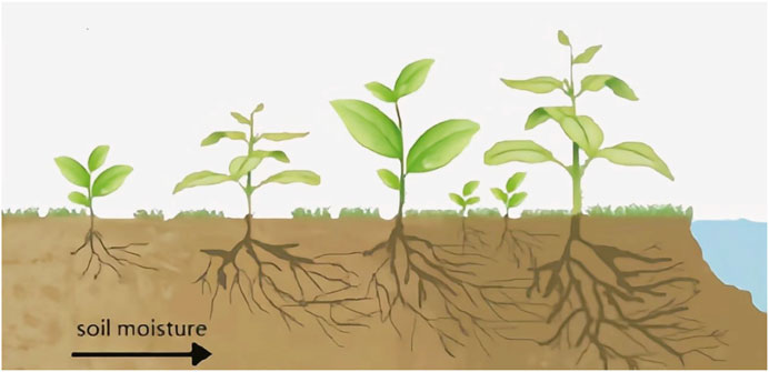
FIGURE 1. Schematic chart of hydrotropism of vegetation roots and the arrow direction indicates that the soil moisture is getting higher and higher. The roots of vegetation grow in areas to obtain more water resources.

The spatial motion of hydrotropism of vegetation roots is to absorb more water. In this sense, it is assumed that the diffusion rate of vegetation hydrotropism is proportional to the diffusion speed of water. Consequently, based on the Klausmeier system [12], we establish a system with water diffusion and vegetation hydrotropism effects as follows:

$\left\{\begin{array}{c}\frac{\partial P}{\partial T}=RJW{P}^2-MP+D_1\mathrm{\Delta }P+D\mathrm{\Delta }W,\hfill \\ \frac{\partial W}{\partial T}=A-RW{P}^2-LW+\xi \frac{\partial W}{\partial X}+D_2\mathrm{\Delta }W,\hfill \end{array}\right.$(2.1)

where P is the vegetation biomass and W is the soil water volume; parameters A, M, L, D₁, D₂ represent rainfall, plant mortality, evaporation rate, vegetation diffusion rate, and water diffusivity, respectively. The term $\xi \frac{\partial W}{\partial X}$ describes the surface runoff which is proportional to the slope of terrain, where ξ is a constant downhill runoff flow velocity, and the term RWP² indicates the absorption of soil moisture by the roots of vegetation, reflecting the mechanism of long-distance inhibition and short-distance promotion [37]. D is the hydrotropism rate of the vegetation.

For the convenience of mathematical analysis, we reduce the numbers of parameters by dimensionless transformation on the system (2.1) and obtain the following system:

$\left\{\begin{array}{c}\frac{\partial p}{\partial t}=w{p}^2-mp+d_1\mathrm{\Delta }p+d\mathrm{\Delta }w,\hfill \\ \frac{\partial w}{\partial t}=a-w\left(1+p^2\right)+\xi \frac{\partial w}{\partial x}+d_2\mathrm{\Delta }w.\hfill \end{array}\right.$(2.2)

In this paper, we mainly study the flat ground without considering the slope’s influence on the formation of the pattern structure. Therefore, our system is finally simplified as follows:

$\left\{\begin{array}{c}\frac{\partial p}{\partial t}=w{p}^2-mp+d_1\mathrm{\Delta }p+d\mathrm{\Delta }w,\hfill \\ \frac{\partial w}{\partial t}=a-w\left(1+p^2\right)+d_2\mathrm{\Delta }w.\hfill \end{array}\right.$(2.3)

2.2 Mathematical analysis of the model

System (2.3) without considering diffusion is as follows:

$\left\{\begin{array}{c}\frac{\mathrm{d}p}{\mathrm{d}t}=w{p}^2-mp,\hfill \\ \frac{\mathrm{d}w}{\mathrm{d}t}=a-w\left(1+p^2\right).\hfill \end{array}\right.$(2.4)

Make the right end of Eq. 2.4 equal to 0, and calculate the equilibrium point. System (2.3) has three equilibrium points, including a semi trivial steady-state solution and two non-trivial steady-state solutions:

(1) E₀ = (p₀, w₀) = (0, a), which corresponds to no vegetation.

(2) $E_1=(p_1,w_1)=(\frac{2m}{a+\sqrt{a^2-4m^2}},\frac{a+\sqrt{a^2-4m^2}}{2})$.

(3) $E_2=(p_2,w_2)=(\frac{2m}{a-\sqrt{a^2-4m^2}},\frac{a-\sqrt{a^2-4m^2}}{2})$.

Because the equilibrium point E₁ is always unstable when diffusion is not considered, we will only study the equilibrium point E₂ given in the following section. First, linearize system (2.3) at E₂ to obtain

$\left\{\begin{array}{c}\frac{\partial p}{\partial t}=a_{11}p+a_{12}w+d_1\mathrm{\Delta }p+d\mathrm{\Delta }w,\hfill \\ \frac{\partial w}{\partial t}=a_{21}p+a_{22}w+d_2\mathrm{\Delta }w,\hfill \end{array}\right.$(2.5)

where

$a_{11}=m,a_{12}=\frac{a+\sqrt{a^2-4m^2}}{a-\sqrt{a^2-4m^2}},a_{21}=-2m,and{a}_{22}=\frac{-2a}{a-\sqrt{a^2-4m^2}}$.

We set a perturbation to the uniform stationary solution (p₂, w₂) and expand it in Fourier space:

$\left(\begin{array}{c}\hfill p\hfill \\ \hfill w\hfill \end{array}\right)=\left(\begin{array}{c}\hfill p_2\hfill \\ \hfill w_2\hfill \end{array}\right)+\sum _k\left(\begin{array}{c}\hfill c_k^1\hfill \\ \hfill c_k^2\hfill \end{array}\right)\exp \left(\lambda t+ikr\right).$(2.6)

Substituting Eq. 2.6 variables into Eq. 2.5, one can obtain its following characteristic equation:

$\begin{array}{ccc}\hfill \left|\begin{array}{cc}\hfill a_{11}-d_1{k}^2-\lambda \hfill & \hfill a_{12}-d{k}^2\hfill \\ \hfill a_{21}\hfill & \hfill a_{22}-d_2{k}^2-\lambda \hfill \end{array}\right|=0.& \hfill & \hfill \end{array}$(2.7)

It is equivalent to the following equation:

${\lambda }^2+T_k\lambda +{△}_k=0,$(2.8)

△_k = a₁₁a₂₂−a₂₁a₁₂+(a₂₁d−(a₁₁d₂+a₂₂d₁))k²+d₁d₂k⁴.

T_k = (d₁+d₂)k²−(a₁₁ + a₂₂).

The characteristic value of system (2.3) is as follows:

${\lambda }_{k,1}=\frac{-T_k+\sqrt{T_k^2-4{△}_k}}{2},{\lambda }_{k,2}=\frac{-T_k-\sqrt{T_k^2-4{△}_k}}{2}$.

Then, necessary conditions for system (2.3) to generate bifurcation behavior are as follows:

$a_{11}+a_{22}=0.$(2.9)

$a_{11}{a}_{22}-a_{12}{a}_{21}-\frac{{\left(a_{11}{d}_2+a_{22}{d}_1-a_{21}d\right)}^2}{4d_1{d}_2}<0.$(2.10)

According to the necessary conditions of Hopf bifurcation (2.9) and Turing bifurcation (2.10), we select a as the control variable, and the system branch diagram of system (2.3) can be drawn, as shown in Figure 2. At the same time, the dispersion relationship of system (2.3) is demonstrated in Figure 3.

FIGURE 2

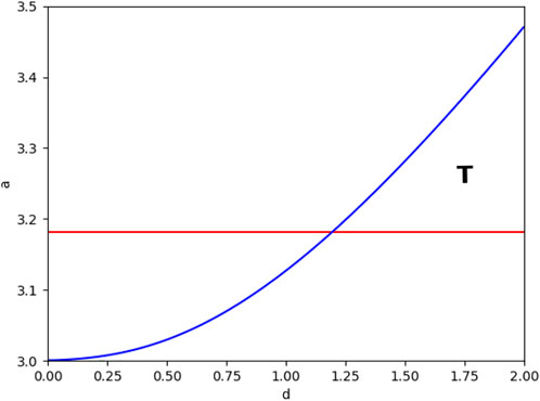
FIGURE 2. Bifurcation diagram of system (2.3) in the parameter space spanned by d and a. Among them, the red line represents the Hopf branch line, and the blue line represents the Turing branch line. The Turing area is marked with T. The parameter values are m = 1.5, d₁ = 1, and d₂ = 1.8.

FIGURE 3

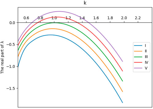
FIGURE 3. Dispersion relation of system (2.3): (I) d = 1, (II) d = 1.2, (III) d = 1.4, (IV) d = 1.6, and (V) d = 1.8. The other parameter values are a = 3.25, m = 1.5, d₁ = 1, and d₂ = 1.8.

Obviously, Figure 3 shows that within an appropriate parameter range, as the parameter d increases, the real part of the eigenvalue gradually increases and the Turing patterns appear.

3 Amplitude equations

Generally, the pattern structure is influenced by the most active mode of the system. The amplitude equation can describe the system’s dynamic behavior around the most active mode [10]. Therefore, we can use the amplitude equation to research the system’s dynamic behavior around the Turing bifurcation point. The pattern structure is represented by three pairs of resonance modes (ν_j, − ν_j), which are 120° angles. For this paper, through the method of multi-scale analysis, the amplitude equation of system (2.3) and its coefficients are derived.

3.1 Multi-scale analysis

First, rewrite system (2.3) at the equilibrium point E₂ as follows:

$\left\{\begin{array}{c}\frac{\partial p}{\partial t}=a_{11}p+a_{12}w+N_1\left(p,w\right)+d_1△p+d△w,\hfill \\ \frac{\partial w}{\partial t}=a_{21}p+a_{22}w+N_2\left(p,w\right)+d_2△w.\hfill \end{array}\right.$(3.1)

Near a = a_T, the solution can be written in the following form:

$\left(\begin{array}{c}\hfill p\hfill \\ \hfill w\hfill \end{array}\right)=\sum _{j=1}^3\left(\begin{array}{c}\hfill A_j^p\hfill \\ \hfill A_j^w\hfill \end{array}\right)\exp \left(i{\nu }_{j}r\right)+c.c.$(3.2)

Making $c=\left(\begin{array}{c}\hfill p\hfill \\ \hfill w\hfill \end{array}\right),N=\left(\begin{array}{c}\hfill N_1\hfill \\ \hfill N_2\hfill \end{array}\right)$, system (3.1) can be written as follows:

$\frac{\partial c}{\partial t}=Lc+N,$(3.3)

where

$L=\left(\begin{array}{cc}\hfill a_{11}+d_1\mathrm{\Delta }\hfill & \hfill a_{12}+d\mathrm{\Delta }\hfill \\ \hfill a_{21}\hfill & \hfill a_{22}+d_2\mathrm{\Delta }\hfill \end{array}\right),N=\left(\begin{array}{c}\hfill \frac{a-\sqrt{a^2-4m^2}}{2}{p}^2+\frac{4m}{a-\sqrt{a^2-4m^2}}pw+p^{2}w\hfill \\ \hfill -\frac{a-\sqrt{a^2-4m^2}}{2}{p}^2-\frac{4m}{a-\sqrt{a^2-4m^2}}pw-p^{2}w\hfill \end{array}\right).$

Expand a, c, L, N as follows:

$\left\{\begin{array}{c}{a}_T-a=\epsilon a_1+{\epsilon }^2{a}_2+\cdots ,\hfill \\ c=\left(\begin{array}{c}\hfill p\hfill \\ \hfill w\hfill \end{array}\right)=\epsilon \left(\begin{array}{c}\hfill p_1\hfill \\ \hfill w_1\hfill \end{array}\right)+{\epsilon }^2\left(\begin{array}{c}\hfill p_2\hfill \\ \hfill w_2\hfill \end{array}\right)+{\epsilon }^3\left(\begin{array}{c}\hfill p_3\hfill \\ \hfill w_3\hfill \end{array}\right)+o\left({\epsilon }^4\right),\hfill \\ L=L_T+\left(a-a_T\right)b,\hfill \\ N={\epsilon }^2{h}^2+{\epsilon }^3{h}^3+o\left({\epsilon }^4\right).\hfill \end{array}\right.$(3.4)

L_T, b, h², h³ are as follows:

$L_T=\left(\begin{array}{cc}\hfill a_{11}^{*}+d_1\mathrm{\Delta }\hfill & \hfill a_{12}^{*}+d\mathrm{\Delta }\hfill \\ \hfill a_{21}^{*}\hfill & \hfill a_{22}^{*}+d_2\mathrm{\Delta }\hfill \end{array}\right)$, $b=\left(\begin{array}{cc}\hfill b_{11}\hfill & \hfill b_{12}\hfill \\ \hfill b_{21}\hfill & \hfill b_{22}\hfill \end{array}\right)$,

$h^2=\left(\begin{array}{c}\hfill (\frac{a-\sqrt{a^2-4m^2}}{2})p_1^2+\frac{4m}{a-\sqrt{a^2-4m^2}}{p}_1{w}_1\hfill \\ \hfill -(\frac{a-\sqrt{a^2-4m^2}}{2})p_1^2-\frac{4m}{a-\sqrt{a^2-4m^2}}{p}_1{w}_1\hfill \end{array}\right)$,

$h^3=\left(\begin{array}{c}\hfill (a-\sqrt{a^2-4m^2})p_1{p}_2+\frac{4m}{a-\sqrt{a^2-4m^2}}(p_1{w}_2+p_2{w}_1)+p_1^2{w}_1\hfill \\ \hfill -(a-\sqrt{a^2-4m^2})p_1{p}_2-\frac{4m}{a-\sqrt{a^2-4m^2}}(p_1{w}_2+p_2{w}_1)-p_1^2{w}_1\hfill \end{array}\right)$.

Decompose the time scale (T = t, T₁ = ɛt, T₂ = ɛ²t), then the derivative of the amplitude A with respect to time is

$\frac{\partial A}{\partial t}=\epsilon \frac{\partial A}{\partial T_1}+{\epsilon }^2\frac{\partial A}{\partial T_2}+\cdots .$(3.5)

Substituting (3.4) into formula (3.3), we get the equation of different order of ɛ (see Table 1).

TABLE 1

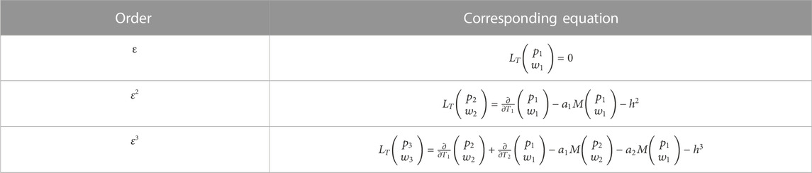
TABLE 1. Equation of different orders of ɛ.

For the order of ɛ,

$\left(\begin{array}{c}\hfill p_1\hfill \\ \hfill w_1\hfill \end{array}\right)L_T=0,$(3.6)

where L_T is the model’s linear operator at the critical point, and $\left(\begin{array}{c}\hfill p_1\hfill \\ \hfill w_1\hfill \end{array}\right)$ is a linear combination of the eigenvectors corresponding to zero eigenvalues of the linear operator L_T. The solution of equation is

$\left(\begin{array}{c}\hfill p_1\hfill \\ \hfill w_1\hfill \end{array}\right)=\sum _{j=1}^3\left(\begin{array}{c}\hfill l\hfill \\ \hfill 1\hfill \end{array}\right)W_j\exp \left(i{\nu }_{j}r\right)+o.o,$(3.7)

with $l=-\frac{a_{22}^{*}{d}_1-a_{11}^{*}{d}_2+a_{21}^{*}d}{2a_{21}^{*}{d}_1},|{\nu }_j|=|{\nu }_T|,{\nu }_T^2=\frac{a_{22}^{*}{d}_1+a_{11}^{*}{d}_2-a_{21}^{*}d}{2d_1{d}_2}$.

For the order of ɛ²,

$L_T\left(\begin{array}{c}\hfill p_2\hfill \\ \hfill w_2\hfill \end{array}\right)=\frac{\partial }{\partial T_1}\left(\begin{array}{c}\hfill p_1\hfill \\ \hfill w_1\hfill \end{array}\right)-a_{1}b\left(\begin{array}{c}\hfill p_1\hfill \\ \hfill w_1\hfill \end{array}\right)-h^2=\left(\begin{array}{c}\hfill F_p\hfill \\ \hfill F_w\hfill \end{array}\right).$(3.8)

According to the solvability condition of Fredholm, to guarantee the existence of equation’s non-trivial solution, the right term of Eq. 3.8 must be the same as the $L_T^{+}$ zero eigenvalue conjugate.

$L_T^{+}=\left(\begin{array}{cc}\hfill a_{11}^{*}-d_1{\nu }_T^2\hfill & \hfill a_{21}^{*}\hfill \\ \hfill a_{12}^{*}-d{\nu }_T^2\hfill & \hfill a_{22}^{*}-d_2{\nu }_T^2\hfill \end{array}\right).$

The zero characteristic value of $L_T^{+}$ is

$\left(\begin{array}{c}\hfill 1\hfill \\ \hfill -\frac{d_1}{d_2}l\hfill \end{array}\right)e^{i{\nu }_{j}r}+o.o.$

Use $F_p^j$ and $F_w^j$ to represent the coefficients corresponding to $e^{i{\nu }_{j}r}$ in F_p and F_w.

$\left\{\begin{array}{c}\left(\begin{array}{c}\hfill F_p^1\hfill \\ \hfill F_w^1\hfill \end{array}\right)=\left(\begin{array}{c}\hfill l\frac{\partial W_1}{\partial T_1}\hfill \\ \hfill \frac{\partial W_1}{\partial T_1}\hfill \end{array}\right)-\left(\begin{array}{c}\hfill \left[\left(a-\sqrt{a^2-4m^2}\right)l^2+\frac{8m}{a-\sqrt{a^2-4m^2}}l\right]{\bar{W}}_3{\bar{W}}_2\hfill \\ \hfill \left[-\left(a-\sqrt{a^2-4m^2}\right)l^2-\frac{8m}{a-\sqrt{a^2-4m^2}}l\right]{\bar{W}}_3{\bar{W}}_2\hfill \end{array}\right)\hfill \\ -a_1\left(\begin{array}{c}\hfill l{b}_{11}{W}_1+b_{12}{W}_1\hfill \\ \hfill l{b}_{21}{W}_1+b_{22}{W}_1\hfill \end{array}\right),\hfill \\ \left(\begin{array}{c}\hfill F_p^2\hfill \\ \hfill F_w^2\hfill \end{array}\right)=\left(\begin{array}{c}\hfill l\frac{\partial W_2}{\partial T_1}\hfill \\ \hfill \frac{\partial W_2}{\partial T_1}\hfill \end{array}\right)-\left(\begin{array}{c}\hfill \left[\left(a-\sqrt{a^2-4m^2}\right)l^2+\frac{8m}{a-\sqrt{a^2-4m^2}}l\right]{\bar{W}}_1{\bar{W}}_3\hfill \\ \hfill \left[-\left(a-\sqrt{a^2-4m^2}\right)l^2-\frac{8m}{a-\sqrt{a^2-4m^2}}l\right]{\bar{W}}_1{\bar{W}}_3\hfill \end{array}\right)\hfill \\ -a_1\left(\begin{array}{c}\hfill l{b}_{11}{W}_2+b_{12}{W}_2\hfill \\ \hfill l{b}_{21}{W}_2+b_{22}{W}_2\hfill \end{array}\right),\hfill \\ \left(\begin{array}{c}\hfill F_p^3\hfill \\ \hfill F_w^3\hfill \end{array}\right)=\left(\begin{array}{c}\hfill l\frac{\partial W_1}{\partial T_3}\hfill \\ \hfill \frac{\partial W_1}{\partial T_3}\hfill \end{array}\right)-\left(\begin{array}{c}\hfill \left[\left(a-\sqrt{a^2-4m^2}\right)l^2+\frac{8m}{a-\sqrt{a^2-4m^2}}l\right]{\bar{W}}_1{\bar{W}}_2\hfill \\ \hfill \left[-\left(a-\sqrt{a^2-4m^2}\right)l^2-\frac{8m}{a-\sqrt{a^2-4m^2}}l\right]{\bar{W}}_1{\bar{W}}_2\hfill \end{array}\right)\hfill \\ -a_1\left(\begin{array}{c}\hfill l{b}_{11}{W}_3+b_{12}{W}_3\hfill \\ \hfill l{b}_{21}{W}_3+b_{22}{W}_3\hfill \end{array}\right),\hfill \end{array}\right.$(3.9)

where $l=-\frac{a_{22}^{*}{d}_1-a_{11}^{*}{d}_2+a_{21}^{*}d}{2a_{21}^{*}{d}_1}$. According to the conjugation condition,

$\left(\begin{array}{cc}\hfill 1,\hfill & \hfill -\frac{d_1}{d_2}l\hfill \end{array}\right)\left(\begin{array}{c}\hfill F_p^j\hfill \\ \hfill F_w^j\hfill \end{array}\right)=0.$

Then,

$\left\{\begin{array}{c}\left(1-\frac{d_1}{d_2}\right)l\frac{\partial W_1}{\partial T_1}=a_1\left[l{b}_{11}+b_{12}-\frac{d_1}{d_2}l\left(l{b}_{21}+b_{22}\right)\right]W_1+\left(1+\frac{d_1}{d_2}\right)\hfill \\ \left[\left(a-\sqrt{a^2-4m^2}\right)l^2+\frac{8ml}{a-\sqrt{a^2-4m^2}}\right]{\bar{W}}_3{\bar{W}}_2,\hfill \\ \left(1-\frac{d_1}{d_2}\right)l\frac{\partial W_2}{\partial T_1}=a_1\left[l{b}_{11}+b_{12}-\frac{d_1}{d_2}l\left(l{b}_{21}+b_{22}\right)\right]W_2+\left(1+\frac{d_1}{d_2}\right)\hfill \\ \left[\left(a-\sqrt{a^2-4m^2}\right)l^2+\frac{8ml}{a-\sqrt{a^2-4m^2}}\right]{\bar{W}}_1{\bar{W}}_3,\hfill \\ \left(1-\frac{d_1}{d_2}\right)l\frac{\partial W_3}{\partial T_1}=a_1\left[l{b}_{11}+b_{12}-\frac{d_1}{d_2}l\left(l{b}_{21}+b_{22}\right)\right]W_3+\left(1+\frac{d_1}{d_2}\right)\hfill \\ \left[\left(a-\sqrt{a^2-4m^2}\right)l^2+\frac{8ml}{a-\sqrt{a^2-4m^2}}\right]{\bar{W}}_1{\bar{W}}_2.\hfill \end{array}\right.$(3.10)

It can be found that the second-order term’s coefficient value is more than 0 from all the aforementioned equations, which will cause the amplitude of W_j to diverge, and higher-order terms need to be introduced to saturate it. Therefore, the solution of Equation 3.8 is written in the following form:

$\begin{array}{ll}\hfill \left(\begin{array}{c}\hfill p_2\hfill \\ \hfill w_2\hfill \end{array}\right)& =\left(\begin{array}{c}\hfill P_0\hfill \\ \hfill W_0\hfill \end{array}\right)+\sum _{j=1}^3\left(\begin{array}{c}\hfill P_j\hfill \\ \hfill W_j\hfill \end{array}\right)e^{i{\nu }_{j}r}+\sum _{j=1}^3\left(\begin{array}{c}\hfill P_{jj}\hfill \\ \hfill W_{jj}\hfill \end{array}\right)e^{i2{\nu }_{j}r}+\left(\begin{array}{c}\hfill P_{12}\hfill \\ \hfill W_{12}\hfill \end{array}\right)e^{ir\left({\nu }_1-{\nu }_2\right)}\hfill \\ \hfill & +\left(\begin{array}{c}\hfill P_{23}\hfill \\ \hfill W_{23}\hfill \end{array}\right)e^{ir\left({\nu }_2-{\nu }_3\right)}+\left(\begin{array}{c}\hfill P_{31}\hfill \\ \hfill W_{31}\hfill \end{array}\right)e^{ir\left({\nu }_3-{\nu }_1\right)}+o.o.\left(j=\mathrm{1,2,3}\right).\hfill \end{array}$(3.11)

Substituting formula (3.11) into Eq. 3.8, we get

$\left(\begin{array}{c}\hfill P_0\hfill \\ \hfill W_0\hfill \end{array}\right)=\left(\begin{array}{c}\hfill p_0\hfill \\ \hfill w_0\hfill \end{array}\right){\sum }_{i=1}^3|W_i{|}^2$, P_i = lW_i,

$\left(\begin{array}{c}\hfill P_{jj}\hfill \\ \hfill W_{jj}\hfill \end{array}\right)=\left(\begin{array}{c}\hfill p_{11}\hfill \\ \hfill w_{11}\hfill \end{array}\right)W_j^2$, $\left(\begin{array}{c}\hfill P_{jk}\hfill \\ \hfill W_{jk}\hfill \end{array}\right)=\left(\begin{array}{c}\hfill p_{*}\hfill \\ \hfill w_{*}\hfill \end{array}\right)W_j{\bar{W}}_k$,

$J=(a-\sqrt{a^2-4m^2})l^2+\frac{8ml}{a-\sqrt{a^2-4m^2}}$,

$p_0=\frac{1}{a_{11}^{*}{a}_{22}^{*}-a_{12}^{*}{a}_{21}^{*}}[(a_{12}^{*}+a_{22}^{*})J]$,

$w_0=\frac{1}{a_{11}^{*}{a}_{22}^{*}-a_{12}^{*}{a}_{21}^{*}}[-(a_{11}^{*}+a_{21}^{*})J]$,

$p_{11}=\frac{1}{(a_{11}^{*}-4d_1{\nu }_T^2)(a_{22}^{*}-4d_2{\nu }_T^2)-a_{21}^{*}(a_{12}-4d{\nu }_T^2)}[-\frac{1}{2}(4d{\nu }_T^2+4d_2{\nu }_T^2-a_{12}^{*}-a_{22}^{*})J]$,

$w_{11}=\frac{1}{(a_{11}^{*}-4d_1{\nu }_T^2)(a_{22}^{*}-4d_2{\nu }_T^2)-a_{21}^{*}(a_{12}^{*}-4d{\nu }_T^2)}[-\frac{1}{2}(a_{21}^{*}+a_{11}^{*}-4d_1{\nu }_T^2)J]$,

$p_{*}=\frac{1}{(a_{11}^{*}-3d_1{\nu }_T^2)(a_{22}^{*}-3d_2{\nu }_T^2)-a_{21}^{*}(a_{12}-3d{\nu }_T^2)}[-(3d{\nu }_T^2+3d_2{\nu }_T^2-a_{12}^{*}-a_{22}^{*})J]$,

$w_{*}=\frac{1}{(a_{11}^{*}-3d_1{\nu }_T^2)(a_{22}^{*}-3d_2{\nu }_T^2)-a_{21}^{*}(a_{12}^{*}-3d{\nu }_T^2)}[-(a_{21}^{*}+a_{11}^{*}-3d_1{\nu }_T^2)J]$.

For the order of ɛ³,

$\begin{array}{ll}\hfill L_T\left(\begin{array}{c}\hfill p_3\hfill \\ \hfill w_3\hfill \end{array}\right)& =\frac{\partial }{\partial T_1}\left(\begin{array}{c}\hfill p_2\hfill \\ \hfill w_2\hfill \end{array}\right)+\frac{\partial }{\partial T_2}\left(\begin{array}{c}\hfill p_1\hfill \\ \hfill w_1\hfill \end{array}\right)-a_{1}b\left(\begin{array}{c}\hfill p_2\hfill \\ \hfill w_2\hfill \end{array}\right)-a_{2}b\left(\begin{array}{c}\hfill p_1\hfill \\ \hfill w_1\hfill \end{array}\right)-h^3\hfill \\ \hfill & =\left(\begin{array}{c}\hfill H_p\hfill \\ \hfill H_w\hfill \end{array}\right).\hfill \end{array}$(3.12)

Similarly, use $H_p^j$ and $H_w^j$ to represent the coefficients corresponding to $e^{i{\nu }_{j}r}$ in H_p and H_w.

$\begin{array}{ll}\hfill \left(\begin{array}{c}\hfill H_p^1\hfill \\ \hfill H_w^1\hfill \end{array}\right)& =\left(\begin{array}{c}\hfill l\frac{\partial V_1}{\partial T_1}\hfill \\ \hfill \frac{\partial V_1}{\partial T_1}\hfill \end{array}\right)+\left(\begin{array}{c}\hfill l\frac{\partial W_1}{\partial T_2}\hfill \\ \hfill \frac{\partial W_1}{\partial T_2}\hfill \end{array}\right)-a_2\left(\begin{array}{c}\hfill l{b}_{11}{W}_1+b_{12}{w}_1\hfill \\ \hfill l{b}_{21}{W}_1+b_{22}{w}_1\hfill \end{array}\right)-a_1\left(\begin{array}{c}\hfill l{b}_{11}{V}_1+b_{12}{V}_1\hfill \\ \hfill l{b}_{21}{V}_1+b_{22}{V}_1\hfill \end{array}\right)\hfill \\ \hfill & -\left(\begin{array}{c}\hfill -K|W_1{|}^2-L\left(|W_2{|}^2-|W_3{|}^2\right)\hfill \\ \hfill K|W_1{|}^2+L\left(|W_2{|}^2-|W_3{|}^2\right)\hfill \end{array}\right)W_1\hfill \\ \hfill & +\left(\begin{array}{c}\hfill -\left(a-\sqrt{a^2-4m^2}\right)l^2-\frac{4ml}{a-\sqrt{a^2-4m^2}}\hfill \\ \hfill \left(a-\sqrt{a^2-4m^2}\right)l^2+\frac{4ml}{a-\sqrt{a^2-4m^2}}\hfill \end{array}\right)\left({\bar{W}}_2{\bar{V}}_3+{\bar{V}}_2{\bar{W}}_3\right),\hfill \end{array}$(3.13)

where

$K=-(a-\sqrt{a^2-4m^2}l(p_{11}+p_0))-\frac{4m}{a-\sqrt{a^2-4m^2}}(l(w_{11}+w_0)+(p_{11}+p_0))-3l^2$ and

$L=-(a-\sqrt{a^2-4m^2}l(p_{*}+p_0))-\frac{4m}{a-\sqrt{a^2-4m^2}}(l(w_{*}+w_0)+(p_{*}+p_0))-6l^2$.

According to the solvability condition of Fredholm, we get

$\begin{array}{ll}\hfill l\left(1-\frac{d_1}{d_2}\right)\left(\frac{\partial W_1}{\partial T_2}+\frac{\partial V_1}{\partial T_1}\right)& =\left(a_1{V}_1+a_2{W}_1\right)\left[l{b}_{11}+b_{12}-l\frac{d_1}{d_2}\left(l{b}_{21}+b_{22}\right)\right]\hfill \\ \hfill & -W_1\sum _{i=1}^2{G}_i|W_i{|}^2-W_1|W_3{|}^2\hfill \\ \hfill & +\left(1+\frac{d_1}{d_2}\right)P\left({\bar{W}}_2{\bar{V}}_3+{\bar{W}}_3{\bar{V}}_2\right),\hfill \end{array}$(3.14)

where $G_1=(1+\frac{d_1}{d_2})K$ and $G_2=(1+\frac{d_1}{d_2})L$.

Change the subscript to get the other equation. Then, the amplitude M_i can be expressed as follows:

$M_i=\epsilon W_i+{\epsilon }^2{U}_i+o\left({\epsilon }^3\right).$(3.15)

Combine Eqs 3.10, 3.14, 3.15 to get the following amplitude equation:

${ϵ}_0\frac{\partial M_1}{\partial T_t}=\mu M_1+h{\bar{M}}_2{\bar{M}}_3-g_2{M}_1|M_2{|}^2-g_2{M}_1|M_3{|}^2-g_1{M}_1|M_1{|}^2,$(3.16)

where

$\mu =\frac{a_T-a}{a_T}$,

${ϵ}_0=\frac{l(1-\frac{d_1}{d_2})}{a_T[l{b}_{11}+b_{12}-l\frac{d_1}{d_2}(l{b}_{21}+b_{22})]}$,

$g_1=\frac{G_1}{a_T[l{b}_{11}+b_{12}-l\frac{d_1}{d_2}(l{b}_{21}+b_{22})]}$,

$g_2=\frac{G_2}{a_T[l{b}_{11}+b_{12}-l\frac{d_1}{d_2}(l{b}_{21}+b_{22})]}$, and

$h=\frac{((a-\sqrt{a^2-4m^2})l^2+\frac{8ml}{a-\sqrt{a^2-4m^2}})(1+l\frac{d_1}{d_2})}{a_T[l{b}_{11}+b_{12}-l\frac{d_1}{d_2}(l{b}_{21}+b_{22})]}$.

Change the subscript to get the other equation. Then, the amplitude equation of system (2.3) is

$\left\{\begin{array}{c}{ϵ}_0\frac{\partial M_1}{\partial T_t}=\mu M_1+h{\bar{M}}_2{\bar{M}}_3-g_2{M}_1|M_2{|}^2-g_2{M}_1|M_3{|}^2-g_1{M}_1|M_1{|}^2,\hfill \\ {ϵ}_0\frac{\partial M_2}{\partial T_t}=\mu M_2+h{\bar{M}}_1{\bar{M}}_3-g_2{M}_2|M_1{|}^2-g_2{M}_2|M_3{|}^2-g_1{M}_2|M_2{|}^2,\hfill \\ {ϵ}_0\frac{\partial M_3}{\partial T_t}=\mu M_3+h{\bar{M}}_1{\bar{M}}_2-g_2{M}_3|M_1{|}^2-g_2{M}_3|M_2{|}^2-g_1{M}_3|M_3{|}^2.\hfill \end{array}\right.$(3.17)

3.2 Stability analysis

Each amplitude equation can be expressed into the product of its mode β_i = |M_i| and its corresponding phase angle ψ_i, which is M_i = β_i exp (iψ_i). Substituting it into the amplitude Eq. 3.17, we get

$\left\{\begin{array}{c}{ϵ}_0\frac{\partial {\beta }_1}{\partial T_t}=\mu {\beta }_1+h{\beta }_2{\beta }_3\cos \psi -g_2\left({\beta }_2^2+{\beta }_3^2\right){\beta }_1-g_1{\beta }_1^3,\hfill \\ {ϵ}_0\frac{\partial {\beta }_2}{\partial T_t}=\mu {\beta }_2+h{\beta }_1{\beta }_3\cos \psi -g_2\left({\beta }_1^2+{\beta }_3^2\right){\beta }_2-g_1{\beta }_2^3,\hfill \\ {ϵ}_0\frac{\partial {\beta }_3}{\partial T_t}=\mu {\beta }_3+h{\beta }_1{\beta }_2\cos \psi -g_2\left({\beta }_1^2+{\beta }_2^2\right){\beta }_3-g_1{\beta }_3^3,\hfill \\ {ϵ}_0\frac{\partial \psi }{\partial T_t}=-h\frac{{\beta }_1^2{\beta }_2^2+{\beta }_1^2{\beta }_3^2+{\beta }_2^2{\beta }_3^2}{{\beta }_1{\beta }_2{\beta }_3}\sin \psi ,\hfill \end{array}\right.$(3.18)

where ψ = ψ₁+ψ₂+ψ₃.

The aforementioned system has four solutions, corresponding to four different pattern structures. Table 2 summarizes the stability of the four pattern structures.

TABLE 2

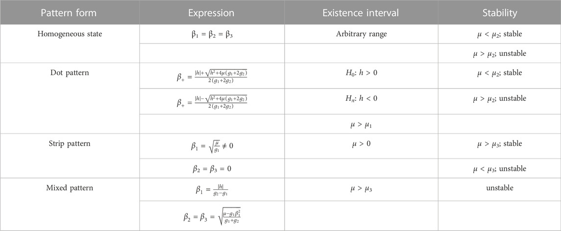
TABLE 2. Equation of different orders of ɛ.

${\mu }_1=\frac{-h^2}{4(g_1+2g_2)}$, μ₂ = 0, ${\mu }_3=\frac{h^2{g}_1}{{(g_2-g_1)}^2}$, and ${\mu }_4=\frac{2g_1+g_2}{{(g_2-2g_1)}^2}{h}^2$.

4 Main results

For the study of the spatial model, we cannot use analytical methods to obtain its dynamic behavior. Therefore, in this section, we simulate system (2.3) using the method of numerical simulation and reveal the influence of vegetation hydrotropism on vegetation growth and distribution. The selected area is M × N, where M = N = 100. Its boundary conditions meet Neumann boundary conditions, that is, the study area is not connected with its surrounding environment. We set the time zone to [0,10000], time step to Δt = 0.1, and spatial step to Δh = 1. The initial value is the random disturbance at the equilibrium point E₂.

4.1 Basic pattern structures

In this part, the theoretical analysis of the third part is verified by numerical simulation. Choose the values of different parameters a, m, d, d₁, and d₂. We can calculate the values of h, g₁, g₂, μ₁, μ₂, μ₃, and μ₄, according to the expression of the amplitude equation coefficients in section 3. In order to observe the simulation results, we have selected three sets of parameter values in Table 3, and the corresponding results are shown in Figure 4; among them, Figure 4 (a₁)-(c₁) is a water pattern and Figure 4 (a₂)-(c₂) is a vegetation pattern. When the first set of parameters is selected, the value of μ is between μ₂ and μ₃, and system (2.3) has a dot pattern, as shown in Figure 4 (a₁) and Figure 4 (a₂); when the second set of parameters is selected, the value of μ is between μ₃ and μ₄, and system (2.3) has a mixed pattern, as shown in Figure 4 (b₁) and Figure 4 (b₂); when the third set of parameters is selected, the value of μ is greater than μ₄, and system (2.3) has a stripe pattern, as shown in Figure 4 (c₁) and Figure 4 (c₂).

TABLE 3

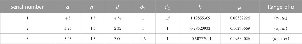
TABLE 3. Different values of parameters.

FIGURE 4

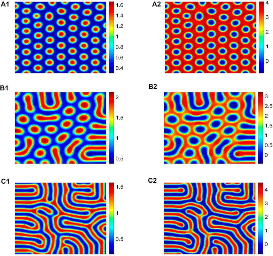
FIGURE 4. For different pattern structures, the parameter values are shown in Table 3. (a₁)-(c₁) is the water pattern, and (a₂)-(c₂) is the vegetation pattern. Among them, (a₁) and (a₂) are spot patterns, (b₁) and (b₂) are mixed patterns, and (c₁) and (c₂) are strip patterns.

4.2. Pattern phase transition induced by soil water diffusion

In this section, we will study the influence of soil water diffusion on vegetation in dry and semi-dry places. In these areas, the lack of water resources causes the diffusion of soil water mainly caused by concentration differences, that is, absorption water feedback. For different vegetation, the ability to absorb water is different, which will lead to the concentration difference of soil water. It is reflected in the parameter d₂ in our model; the greater the concentration difference of soil water, the greater is the parameter d₂. In order to better reveal the effects of different water diffusion intensities on the vegetation pattern, we do not consider the hydrotropism of vegetation and fix the parameters d = 0 and d₁ = 1; then, we can change the parameter d₂ to reflect different water diffusion intensities.

Figure 5 shows the change in the corresponding vegetation pattern with the change in the parameter d₂. With the increase in d₂, the vegetation pattern structures change in the following sequence, gap pattern, mixed pattern, strip pattern, and spot pattern. Moreover, we also find that when d₂ ≤ d₁, no vegetation pattern is generated; when d₂ > d₁, with the increase in the parameter d₂, the gap between the pattern becomes larger and larger. In fact, the difference in the soil water concentration reflects the difference in the water absorption capacity among vegetation. The greater the diffusion intensity of the water beside the vegetation, the stronger is the absorption capacity of the vegetation for water, which will promote its own growth more. Conversely, as the intensity of diffusion of water next to the vegetation increases, more water will flow to its location, which will suppress the growth of the nearby vegetation. It shows that the vegetation pattern is formed through the long-range competition and short-range promotion mechanism.

FIGURE 5

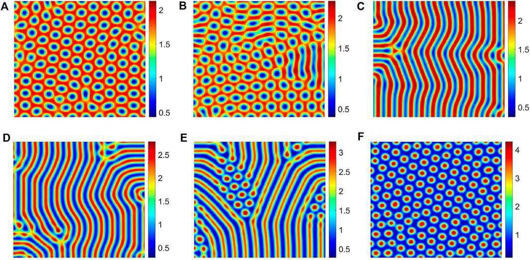
FIGURE 5. Different values of the parameter d₂ correspond to different vegetation patterns, (A) d₂ = 7.80, (B) d₂ = 8.21, (C) d₂ = 9.00, (D) d₂ = 10.20, (E) d₂ = 12.80, and (F) d₂ = 15.48. The other parameter values are a = 3.25, m = 1.50, and d₁ = 1.00.

4.3 Influence of hydrotropism on the vegetation pattern

Due to the climatic conditions and geographical environment in dry and semi-dry regions, the soil water resource distribution is uneven, and a water gradient is formed. Because of the presence of the moisture gradient, roots exhibit hydrotropism characteristics. For different vegetation, the intensity of the hydrotropism of the vegetation root is different. Some vegetation roots are sensitive to soil moisture, but some vegetation roots are relatively weak. Therefore, in this section, we study the influence of different vegetation growth abilities of water on the vegetation in the area. In our spatial model, we fixed other diffusion parameters, that is, d₁ = 1, d₂ = 1, and observed the influence of hydrotropism on the vegetation pattern structures by changing the parameter d. Figure 6 shows the pattern structures of vegetation under different root hydrotropism intensities. Through theoretical analysis and numerical simulation, we know that when we do not consider the hydrotropism of vegetation roots in our model, let d₁ = d₂, in which no vegetation pattern will be generated. Therefore, the hydrotropism of vegetation roots can induce the generation of vegetation patterns.

FIGURE 6

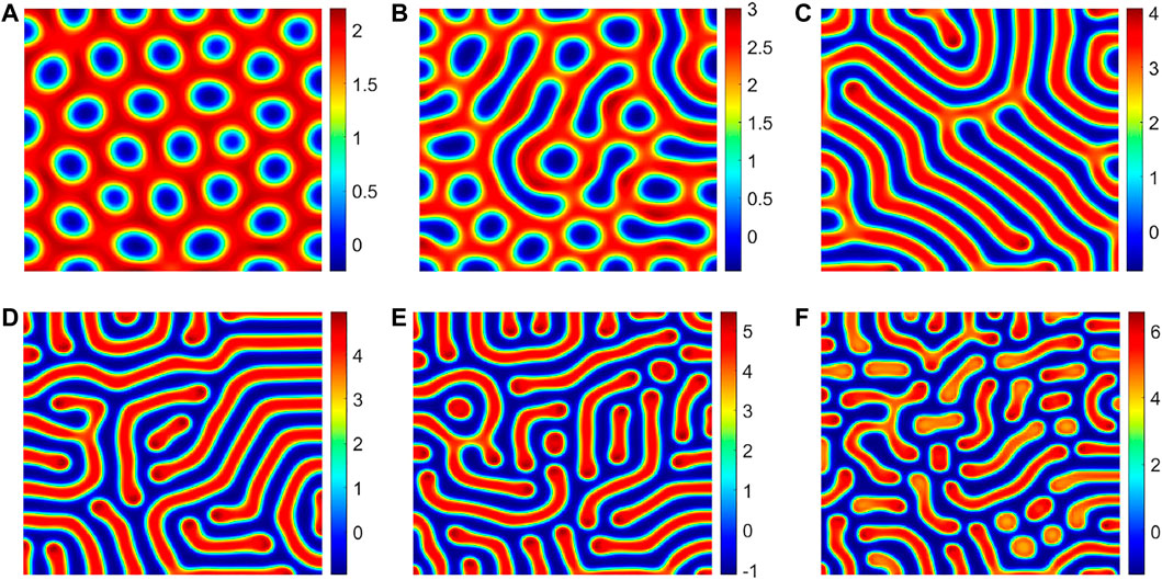
FIGURE 6. Different values of the parameter d correspond to different vegetation patterns, (A) d = 1.52, (B) d = 2.34, (C) d = 3.81, (D) d = 5.86, (E) d = 7.23, and (F) d = 9.56. The other parameter values are a = 3.25, m = 1.5, d₁ = 1, and d₂ = 1.

In Figure 6, we show the influence of the parameter d on the vegetation pattern structures. When the parameter d is small, the gap pattern appears (Figure 6A). When the parameter d increases slightly, the gap pattern begins to disappear, the strip pattern appears, and the vegetation pattern structure becomes mixed gap and strip pattern structures (Figure 6B). When the parameter d continues to increase, the gap pattern completely disappears, showing the strip pattern structure (Figure 6C). Subsequently, with the increase in the d parameter, the spot pattern gradually appears (Figures 6D,F). To sum up, gradually enhance the hydrotropism effect of roots, then the vegetation pattern’s structure changes in the following sequence: the gap pattern, mixed pattern, strip pattern, and spot pattern. In Figure 7, we show the realistic vegetation distribution corresponding to numerical simulation pattern structures.

FIGURE 7

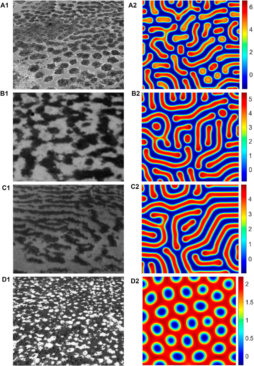
FIGURE 7. Vegetation structure observed in the nature and pattern structure obtained by numerical simulation. Fig (a₁-d₁) shows realistic vegetation pattern structures: (a₁) Zambia, spot vegetation structure [4]; (b₁) Niger, mixed vegetation structure [27]; (c₁) Niamey and Niger, stripe vegetation structure [12]; and (d₁) SW Niger, gap vegetation structure [4]. Fig (a₂-d₂) shows corresponding numerical simulation patterns.

Moreover, in Figure 8, we show the relationship between the root hydrotropism effect and average vegetation biomass. We can find that with the increasing intensity of the hydrotropism of the vegetation root, the average density of vegetation increases. However, as the intensity of vegetation to grow toward water increases, the interval of plants also becomes larger, which means that the stability of the ecosystem in the region is also reduced.

FIGURE 8

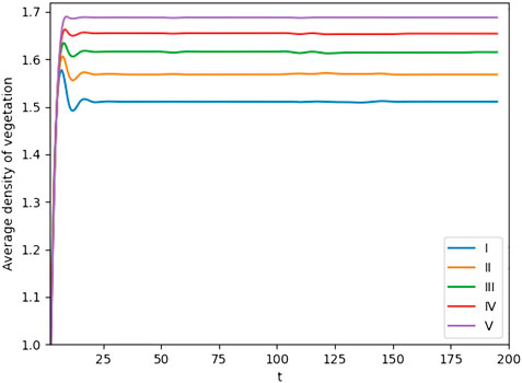
FIGURE 8. Average density of vegetation changes with time t corresponding to different values of the parameter d (I) d = 3.52, (II) d = 4.52, (III) d = 5.52, (IV) d = 6.52, and (V) d = 7.52. The other parameter values are a = 3.25, m = 1.50, d₁ = 1.00, and d₂ = 1.00.

Owing to the fact that water at the location of the vegetation itself is not enough to meet the needs of its own growth, the vegetation has to extend to the humid area to obtain water resources through the roots, which makes the root system of the vegetation exhibit hydrotropism. For different vegetation, the degree of development of the root system is different. When the root system of vegetation is developed, vegetation has higher hydrotropism effects, which means it can absorb more water and other vegetation cannot obtain enough water resources because of limited water resources in these dry regions. A large amount of vegetation died due to the lack of water, resulting in vegetation degradation. In other words, increasing the intensity of the hydrotropism of roots in a range can increase the average biomass of vegetation. However, excessively increasing the intensity of the hydrotropism of roots will lead to desertification.

5 Conclusion

In our paper, we mainly analyze spatial dynamics with hydrotropism effects. First, on the basis of Klausmeier’s system, a spatial system is established considering the hydrophilic effect. Then, the existence and stability of the system equilibrium point are analyzed. Second, through the method of multi-scale analysis, the amplitude equation of the system and its coefficients are derived [38–40]. Finally, we numerically simulated the system to show the influence of vegetation root hydrotropism on vegetation growth distribution.

Bases on the numerical results, we find that the hydrotropism of vegetation roots can induce pattern generation. Furthermore, with the enhancement of the root hydrotropism effect, pattern structures change as follows: the spot pattern, mixed pattern, strip pattern, and gap pattern. Moreover, we also study the relationship between the root hydrotropism effects and average vegetation biomass. We find that increasing the intensity of the hydrotropism of roots in a range can increase the average vegetation biomass which is consistent with the results in [35, 41]. However, excessively increasing the strength of root hydrotropism, the spacing between the vegetation pattern also increases, which means that the ecosystem stability is reduced and prone to land desertification.

We all know that many factors will affect vegetation distribution in the real world, including climatic conditions (such as temperature, light, and carbon dioxide concentration), topographic conditions (such as mountains and plains), and human activities (such as deforestation and grazing) [41–50]. However, in our system, we only consider rainfall and vegetation root hydrotropism effects. Therefore, in order to better protect vegetation, prevent land desertification, and improve the stability of the ecosystem, we hope to establish a more realistic vegetation dynamic system, including climatic conditions, internal growth mechanism of vegetation, human activities, and other factors, to better study the dynamic mechanism of spatial vegetation and reveal relevant factors affecting the structure of the vegetation pattern.

Data availability statement

The original contributions presented in the study are included in the article/Supplementary Material; further inquiries can be directed to the corresponding author.

Author contributions

All authors have made great contributions to the writing of the study and approved the submitted version. LL, F-LW, and L-FH established dynamical modeling, participated in the program design, and provided valuable comments on the manuscript writing.

Funding

The research was supported by the National Key Research and Development Program of China (2018YFE0109600) and the National Natural Science Foundation of China (Nos. 42275034 and 42075029).

Conflict of interest

The authors declare that the research was conducted in the absence of any commercial or financial relationships that could be construed as a potential conflict of interest.

Publisher’s note

All claims expressed in this article are solely those of the authors and do not necessarily represent those of their affiliated organizations, or those of the publisher, the editors, and the reviewers. Any product that may be evaluated in this article, or claim that may be made by its manufacturer, is not guaranteed or endorsed by the publisher.

References

1. Jones CG, Lawton JH, Shachak M. Organisms as ecosystem engineers. In: Ecosystem management. Berlin, Germany: Springer (1994). p. 130–47. doi:10.1007/978-1-4612-4018-1_14

CrossRef Full Text | Google Scholar

2. Jones CG, Lawton JH, Shachak M. Positive and negative effects of organisms as physical ecosystem engineers. Ecology (1997) 78(7):1946–57.

CrossRef Full Text | Google Scholar

3. Shi C, Zhou Y, Fan X, Shao W. A study on the annual runoff change and its relationship with water and soil conservation practices and climate change in the middle yellow river basin. Catena (2013) 100:31–41.

CrossRef Full Text | Google Scholar

4. Wright JP, Jones CG. The concept of organisms as ecosystem engineers ten years on: Progress, limitations, and challenges. BioScience (2006) 56(3):203–9. doi:10.1641/0006-3568(2006)056[0203:tcooae]2.0.co;2

CrossRef Full Text | Google Scholar

5. D’Odorico P, Bhattachan A, Davis KF, Ravi S, Runyan CW. Global desertification: Drivers and feedbacks. Adv Water Resour (2013) 51:326–44.

Google Scholar

6. Sun GQ, Li L, Li L, Liu C, Wu YP, Gao S, et al. Impacts of climate change on vegetation pattern: Mathematical modeling and data analysis. Phys Life Rev (2022) 43:239–70. doi:10.1016/j.plrev.2022.09.005

PubMed Abstract | CrossRef Full Text | Google Scholar

7. Wang Q, Takahashi H. A land surface water deficit model for an arid and semiarid region: Impact of desertification on the water deficit status in the loess plateau, China. J Clim (1999) 12(1):244–57. doi:10.1175/1520-0442-12.1.244

CrossRef Full Text | Google Scholar

8. Saco PM, Willgoose GR, Hancock GR. Eco-geomorphology of banded vegetation patterns in arid and semi-arid regions. Hydrol Earth Syst Sci (2007) 11(6):1717–30. doi:10.5194/hess-11-1717-2007

CrossRef Full Text | Google Scholar

9. Sherratt JA. An analysis of vegetation stripe formation in semi-arid landscapes. J Math Biol (2005) 51(2):183–97. doi:10.1007/s00285-005-0319-5

PubMed Abstract | CrossRef Full Text | Google Scholar

10. Sun GQ, Wang CH, Chang LL, Wu YP, Li L, Jin Z. Effects of feedback regulation on vegetation patterns in semi-arid environments. Appl Math Model (2018) 61:200–15.

CrossRef Full Text | Google Scholar

11. Sherratt JA, Synodinos AD. Vegetation patterns and desertification waves in semi-arid environments: Mathematical models based on local facilitation in plants. DCDS-B (2012) 17(8):2815–27. doi:10.3934/dcdsb.2012.17.2815

CrossRef Full Text | Google Scholar

12. Klausmeier CA. Regular and irregular patterns in semiarid vegetation. Science (1999) 284(5421):1826–8. doi:10.1126/science.284.5421.1826

PubMed Abstract | CrossRef Full Text | Google Scholar

13. von Hardenberg J, Meron E, Shachak M, Zarmi Y. Diversity of vegetation patterns and desertification. Phys Rev Lett (2001) 87(19):198101. doi:10.1103/physrevlett.87.198101

PubMed Abstract | CrossRef Full Text | Google Scholar

14. Gilad E, von Hardenberg J, Provenzale A, Shachak M, Meron E. A mathematical model of plants as ecosystem engineers. J Theor Biol (2007) 244(4):680–91. doi:10.1016/j.jtbi.2006.08.006

PubMed Abstract | CrossRef Full Text | Google Scholar

15. van der Stelt S, Doelman A, Geertje H, Jens Rademacher DM. Rise and fall of periodic patterns for a generalized klausmeier–gray–scott model. J Nonlinear Sci (2013) 23(1):39–95.

Google Scholar

16. Zelnik YR, Meron E, Bel G. Gradual regime shifts in fairy circles. Proc Natl Acad Sci U.S.A (2015) 112(40):12327–31. doi:10.1073/pnas.1504289112

PubMed Abstract | CrossRef Full Text | Google Scholar

17. Bo TL, Fu LT, Zheng XJ. Modeling the impact of overgrazing on evolution process of grassland desertification. Aeolian Res (2013) 9:183–9. doi:10.1016/j.aeolia.2013.01.001

CrossRef Full Text | Google Scholar

18. Chen Z, Wu YP, Feng GL, Qian ZH, Sun GQ. Effects of global warming on pattern dynamics of vegetation: Wuwei in China as a case. Appl Maths Comput (2021) 390:125666. doi:10.1016/j.amc.2020.125666

CrossRef Full Text | Google Scholar

19. Li L, Sun GQ, Guo ZG. Bifurcation analysis of an extended Klausmeier-Gray-Scott model with infiltration delay. Stud Appl Math (2022) 148:1519–42. doi:10.1111/sapm.12482

CrossRef Full Text | Google Scholar

20. Li L, Sun GQ, Jin Z. Interactions of time delay and spatial diffusion induce the periodic oscillation of the vegetation system. DCDS-B (2022) 27:2147–72. doi:10.3934/dcdsb.2021127

CrossRef Full Text | Google Scholar

21. Liu C, Li L, Wang Z, Wang R. Pattern transitions in a vegetation system with cross-diffusion. Appl Maths Comput (2019) 342:255–62. doi:10.1016/j.amc.2018.09.039

CrossRef Full Text | Google Scholar

22. Sherratt JA, Lord GJ. Nonlinear dynamics and pattern bifurcations in a model for vegetation stripes in semi-arid environments. Theor Popul Biol (2007) 71(1):1–11. doi:10.1016/j.tpb.2006.07.009

PubMed Abstract | CrossRef Full Text | Google Scholar

23. Sun GQ, Zhang HT, Song YL, Li L, Jin Z. Dynamic analysis of a plant-water model with spatial diffusion. J Differential Equations (2022) 329:395–430. doi:10.1016/j.jde.2022.05.009

CrossRef Full Text | Google Scholar

24. Tarnita C, Bonachela JA, Sheffer E, Guyton JA, Coverdale TC, Long RA, et al. A theoretical foundation for multi-scale regular vegetation patterns. Nature (2017) 541(7637):398–401. doi:10.1038/nature20801

PubMed Abstract | CrossRef Full Text | Google Scholar

25. Xue Q, Sun GQ, Liu C, Guo Z, Jin Z, Wu YP, et al. Spatiotemporal dynamics of a vegetation model with nonlocal delay in semi-arid environment. Nonlinear Dyn (2020) 99(4):3407–20. doi:10.1007/s11071-020-05486-w

CrossRef Full Text | Google Scholar

26. Chen S, Li J, Wang S, Fritz E, Hüttermann A, Altman A. Effects of nacl on shoot growth, transpiration, ion compartmentation, and transport in regenerated plants of populus euphratica and populus tomentosa. Can J For Res (2003) 33(6):967–75. doi:10.1139/x03-066

CrossRef Full Text | Google Scholar

27. Lin H, Chen Y, Zhang H, Fu P, Fan Z. Stronger cooling effects of transpiration and leaf physical traits of plants from a hot dry habitat than from a hot wet habitat. Funct Ecol (2017) 31(12):2202–11. doi:10.1111/1365-2435.12923

CrossRef Full Text | Google Scholar

28. Hille Ris Lambers R, Rietkerk M, van den Bosch F, Prins HHT, de Kroon H. Vegetation pattern formation in semi-arid grazing systems. Ecology (2001) 82(1):50–61. doi:10.1890/0012-9658(2001)082[0050:vpfisa]2.0.co;2

CrossRef Full Text | Google Scholar

29. Takahashi H. Hydrotropism: The current state of our knowledge. J Plant Res (1997) 110(2):163–9. doi:10.1007/bf02509304

PubMed Abstract | CrossRef Full Text | Google Scholar

30. Takahashi H, Miyazawa Y, Fujii N. Hormonal interactions during root tropic growth: Hydrotropism versus gravitropism. Plant Mol Biol (2009) 69(4):489–502. doi:10.1007/s11103-008-9438-x

PubMed Abstract | CrossRef Full Text | Google Scholar

31. Takahashi N, Yamazaki Y, Kobayashi A, Higashitani A, Takahashi H. Hydrotropism interacts with gravitropism by degrading amyloplasts in seedling roots of arabidopsis and radish. Plant Physiol (2003) 132(2):805–10. doi:10.1104/pp.018853

PubMed Abstract | CrossRef Full Text | Google Scholar

32. Gómez-Plaza A, Martınez-Mena M, Albaladejo J, Castillo VM. Factors regulating spatial distribution of soil water content in small semiarid catchments. J Hydrol (2001) 253(1-4):211–26. doi:10.1016/s0022-1694(01)00483-8

CrossRef Full Text | Google Scholar

33. Wu GL, Zhang ZN, Wang D, Shi ZH, Zhu YJ. Interactions of soil water content heterogeneity and species diversity patterns in semi-arid steppes on the loess plateau of China. J Hydrol (2014) 519:1362–7. doi:10.1016/j.jhydrol.2014.09.012

CrossRef Full Text | Google Scholar

34. Dietrich D. Hydrotropism: How roots search for water. J Exp Bot (2018) 69(11):2759–71. doi:10.1093/jxb/ery034

PubMed Abstract | CrossRef Full Text | Google Scholar

35. Liu C, Wang FG, Xue Q, Li L, Wang Z. Pattern formation of a spatial vegetation system with root hydrotropism. Appl Maths Comput (2022) 420:126913. doi:10.1016/j.amc.2021.126913

CrossRef Full Text | Google Scholar

36. Miyazawa Y, Takahashi A, Kobayashi A, Kaneyasu T, Fujii N, Takahashi H. GNOM-mediated vesicular trafficking plays an essential role in hydrotropism of arabidopsis roots. Plant Physiol (2009) 149(2):835–40. doi:10.1104/pp.108.131003

PubMed Abstract | CrossRef Full Text | Google Scholar

37. Wang X, Zhang G. Vegetation pattern formation in seminal systems due to internal competition reaction between plants. J Theor Biol (2018) 458:10–4. doi:10.1016/j.jtbi.2018.08.043

PubMed Abstract | CrossRef Full Text | Google Scholar

38. Guo ZG, Sun GQ, Wang Z, Jin Z, Li L, Li C. Spatial dynamics of an epidemic model with nonlocal infection. Appl Maths Comput (2020) 377:125158. doi:10.1016/j.amc.2020.125158

CrossRef Full Text | Google Scholar

39. Liang J, Liu C, Sun GQ, Li L, Zhang L, Hou M, et al. Nonlocal interactions between vegetation induce spatial patterning. Appl Maths Comput (2022) 428:127061. doi:10.1016/j.amc.2022.127061

CrossRef Full Text | Google Scholar

40. Liu QX, Herman MJ, Mooij WM, Huisman J, Scheffer M, Olff O, et al. Pattern formation at multiple spatial scales drives the resilience of mussel bed ecosystems. Nat Commun (2014) 5(1):5234–7. doi:10.1038/ncomms6234

PubMed Abstract | CrossRef Full Text | Google Scholar

41. Xue Q, Liu C, Li L, Sun GQ, Wang Z. Interactions of diffusion and nonlocal delay give rise to vegetation patterns in semi-arid environments. Appl Maths Comput (2021) 399:126038. doi:10.1016/j.amc.2021.126038

CrossRef Full Text | Google Scholar

42. Baldi G, Verón SR, Jobbágy EG. The imprint of humans on landscape patterns and vegetation functioning in the dry subtropics. Glob Change Biol (2013) 19(2):441–58. doi:10.1111/gcb.12060

PubMed Abstract | CrossRef Full Text | Google Scholar

43. Bonachela JA, Pringle RM, Sheffer E, Coverdale TC, Guyton JA, Caylor K, et al. Termite mounds can increase the robustness of dryland ecosystems to climatic change. Science (2015) 347(6222):651–5. doi:10.1126/science.1261487

PubMed Abstract | CrossRef Full Text | Google Scholar

44. Kéfi S, Rietkerk M, Alados AL, Pueyo Y, Papanastasis VP, ElAich E, et al. Spatial vegetation patterns and imminent desertification in mediterranean arid ecosystems. Nature (2007) 449(7159):213–7. doi:10.1038/nature06111

PubMed Abstract | CrossRef Full Text | Google Scholar

45. Kefi S, Rietkerk M, Katul GG. Vegetation pattern shift as a result of rising atmospheric co2 in arid ecosystems. Theor Popul Biol (2008) 74(4):332–44. doi:10.1016/j.tpb.2008.09.004

PubMed Abstract | CrossRef Full Text | Google Scholar

46. Lawley V, Parrott L, Lewis MR, Sinclair B, Ostendorf B. Self-organization and complex dynamics of regenerating vegetation in an arid ecosystem: 82 years of recovery after grazing. J Arid Environments (2013) 88:156–64. doi:10.1016/j.jaridenv.2012.08.014

CrossRef Full Text | Google Scholar

47. Marasco A, Iuorio A, Cartení F, Bonanomi G, Tartakovsky MT, Mazzoleni S, et al. Vegetation pattern formation due to interactions between water availability and toxicity in plant-soil feedback. Bull Math Biol (2014) 76(11):2866–83. doi:10.1007/s11538-014-0036-6

PubMed Abstract | CrossRef Full Text | Google Scholar

48. Meron E, Gilad E, von Hardenberg J, Shachak M, Zarmi Y. Vegetation patterns along a rainfall gradient. Chaos, Solitons & Fractals (2004) 19(2):367–76. doi:10.1016/s0960-0779(03)00049-3

CrossRef Full Text | Google Scholar

49. Sun GQ, Zhang HT, Wang JS, Li L, Wang Y, Li L, et al. Mathematical modeling and mechanisms of pattern formation in ecological systems: A review. Nonlinear Dyn (2021) 104(2):1677–96. doi:10.1007/s11071-021-06314-5

CrossRef Full Text | Google Scholar

50. Zhang HT, Wu YP, Sun GQ, Liu C, Feng GL. Bifurcation analysis of a spatial vegetation model. Appl Maths Comput (2022) 434:127459. doi:10.1016/j.amc.2022.127459

CrossRef Full Text | Google Scholar