 Rui-Jie Wu1
 Yi-Cheng Zhang
 Gui-Yuan Shi
95% of researchers rate our articles as excellent or good
Learn more about the work of our research integrity team to safeguard the quality of each article we publish.
Find out more
ORIGINAL RESEARCH article
Front. Phys. , 14 December 2022
Sec. Interdisciplinary Physics
Volume 10 - 2022 | https://doi.org/10.3389/fphy.2022.1076314
This article is part of the Research Topic Complex Networks in Interdisciplinary Research: From Theory to Applications View all 12 articles
Multiplex networks are generally considered as networks that have the same set of vertices but different types of edges. Multiplex networks are especially useful when describing systems with several kinds of interactions. In this paper, we study the analytical solution of the k-core pruning process on multiplex networks. k-Core decomposition is a widely used method to find the dense core of the network. Previously, the Non-Backtracking Expansion Branch (NBEB) has been found to be able to easily derive the exact analytical results in the k-core pruning process. Here, we further extend this method to solve the k-core pruning process on multiplex networks by designing a variation of the method called the Multicolor Non-Backtracking Expansion Branch (MNEB). Our results show that, given any uncorrelated multiplex network, the Multicolor Non-Backtracking Expansion Branch can offer the exact solution for each intermediate state of the pruning process.
Graphs are often used to model systems that consist of interacting people or entities, where the vertices represent people or entities and the edges represent connections. Nowadays, many graphs are built in this way, from a variety of systems and applications, such as online social networks, e-commerce platforms, and even protein interaction networks. One of the most important tasks in analyzing these graphs is to find the densest part of the network where the vertices are closely related to each other [1–4]. The most commonly used algorithm for this problem is called the k-core decomposition [5], in which the goal is to find the subgraph consisting of the vertices that are left after all vertices whose degrees less than k are removed. k-Core decomposition is widely used to identify the important nodes of networks [6–8], help visualize network structures [9,10], understand and explain the collaborative process in social networks [11,12], describe protein functions based on protein–protein networks [13,14], and promote network methods for large text summaries [15].
Previously, many researchers [12,16–18] have focused on solving the k-core decomposition problem on a single-layer network. Wu [19] showed that the Non-Backtracking Expansion Branch can be used to obtain the exact results of the k-core pruning process on single-layer networks. The Non-Backtracking Expansion Branch is an alternative representation to the usual adjacency matrix of a network, which is constructed as an infinite tree having the same local structural information as the given network when observed by non-backtracking walkers.
These findings are important for our understanding of the structure of complex networks. Meanwhile, in real-world scenarios, it is common that we have to deal with systems that consist of many different types of interactions. As a result, systems cannot be represented by a single-layer network. For systems with multiple kinds of connections, we naturally use multiplex networks [20] that have the same set of vertices but different kinds of edges to represent these systems. Multiplex networks are also called multirelational networks, in which the edges between vertices can represent several different types of interactions. These multiplex networks can be used to describe real networks [21] or dynamic processes [22]. In recent years, there has been a trend in network research to study k-kernels on multiplexed networks. Azimi-Tafreshi [23] derived the self-consistent equation, obtained the birth point and relative size of the k-core of the uncorrelated multiplex networks with arbitrary degree distribution, and found hybrid phase transition. Subsequently, by analyzing different real multiplex networks, Osat [24] proposed a new multiplex network model and showed that interlayer correlations are important in characterizing their k-core structure, that is, the organization in the shell layers of nodes with increasing degrees. Radicchi [25]found that for larger numbers of layers, adding new layers increases the robustness of the system by creating redundant interdependencies between layers. Shang [26] revealed that there is a tipping point in the number of layers beyond which the multilayer k-core suddenly collapses. Boccaletti [20] proposed a comprehensive overview of the organization and dynamics between the components (layers) is given and several related issues are covered, ranging from a complete redefinition of fundamental structural measures to understanding how the multilayered nature of networks affects processes and dynamics. In a multiplex network, each kind of connection is represented by a unique layer, and the same vertex is allowed to have different network structures in different layers. Figures 1A–C show a simple example of a multiplex network.
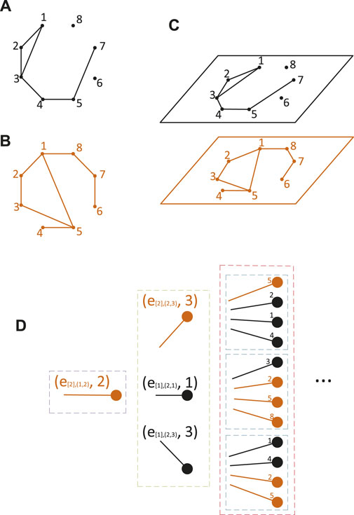
FIGURE 1. Example of a two-layer network. (A) First layer; (B) second layer; (C) two-layer network consists of the two layers (A) and (B). (D) Multicolor Non-Backtracking Expansion Branch B(e[2],(1,2), 2)of the two-layer network is shown (B). Here, e[h],(i,j) denotes the edge that connects the vertex i and vertex j in the hth layer. The purple, green, and red boxes represent the first, second, and third strata of the MNEB, respectively. It should be noted that the excess neighbor stub set S(e[2],(1,2), 2) = {(e[2],(2,3), 3), (e[1],(2,1), 1), (e[1],(2,3), 3)}. The child stubs of the stub (e[2],(1,2), 2) are all the elements in S(e[2],(1,2), 2), as shown in the green box. The three blue boxes represent the child stubs of the three corresponding stubs in the second stratum, respectively.
These existing papers show that both intra-layer and inter-layer correlations have important effects on k-core phase transition. For a long time, due to the lack of mathematical tools, theoretical analysis of the k-core process on multiplex networks has been rare. Here, we show that by assigning different colors to distinguish the types of interactions, we can use the Multicolor Non-Backtracking Expansion Branch (MNEB) method to analytically obtain the results of each step in the k-core pruning process in a multiplex network.
k-Core decomposition on multiplex networks is used to find the largest subgraph in which the degree of each vertex is at least ki in the ith layer (here k is a non-negative integral vector). In the previous paper [23], the researchers gave the analytical result of the final size of the k-core on multiplex networks. Here, we show that the Non-Backtracking Expansion Branch (NBEB) method can be used to obtain the complete solution of k-core decomposition on the multiplex, in which not only the final state but also each intermediate state of the pruning process can be obtained analytically.
Given a multiplex network in which each layer is a simple graph, the standard pruning algorithm for k-core decomposition is as follows: for a given sequence of ki, at each step, we remove these nodes whose degrees in any of these layers are less than the corresponding k. In the following, we analyze, in detail, the pruning process and attempt to give the size of the remaining vertices after each step.
First of all, we introduce the definitions of the terms that are used in the remainder of the paper. Suppose a given multiplex network has R layers. For convenience, we assign each layer with a color ci to distinguish the edges that belong to different network layers. A “stub” is defined as a combination of an edge e[i] and one of its end vertex V, denoted by (e[i], V), where the subscript [i] here means that it belongs to the ith layer, and i can be any integer in [1, R]. Obviously, the stub (e[i], V) has the color ci. We denote by ki the degree of the vertex V in the ith layer. In the ith layer, we define the neighbor stub set of the vertex V:
Consequently, for the whole multiplex network, we define the neighbor stub set of the vertex V as
and the excess neighbor stub set of (e[i], V) as
It should be noted that the aforementioned expression of the excess neighbor stub set S(e[i], V) is equivalent to the complementary set of {(e[i], V*)} in S(V).
Similar to the definition of the Non-Backtracking Expansion Branch (NBEB) in one layer network, starting from any stub (e[i], V), we can define such a tree-like structure, which we call the Multicolor Non-Backtracking Expansion Branch(MNEB).
The chosen stub (e[i], V) (with color ci) is the root of the MNEB, regarded as the first stratum. For any known nth stratum of the MNEB, we can further find the child stubs of each stub in the nth stratum that are all the elements in its excess neighbor stub set, and all these child stubs constitute the (n+1)th stratum of the MNEB. For example, if we have a stub
For a given R-dimensional positive integral vector k = (k1, k2, …, kR), we can find a set of MNEBs Y[i],n (n is a positive integer) for each 1 ≤ i ≤ R that meet the following two conditions: 1. the root of the MNEB is colored with ci; 2. there exists a sub-branch of the MNEB that contains the root stub; for each vertex colored with cj in the first n strata of this sub-branch, it has at least kj−1 child vertices colored with cj and at least kl child vertices colored with cl for every l ≠ j(1 ≤ l ≤ R). Figure 2 shows the details of how to decide whether an MNEB belongs to Y[i],n. When n = 0, for each 1 ≤ i ≤ R, we define Y[i],0 as all the MNEBs whose roots are colored with ci. Obviously, Y[i],0 ⊃ Y[i],1 ⊃⋯ ⊃ Y[i],n ⊃… . We denote SMNEB(V) as the set of MNEBs of all the stubs in S(V) and SMNEB(e[i], V) as the set of MNEBs of all the stubs in S(e[i], V). It is easy to obtain the following theorem from the definition of Y[i],n:

FIGURE 2. Graphic illustration of Y[1],n of the two-layer network shown in Figure 1. The MNEB B(e[1],(1,3), 3) has the root colored with c1 = black. For example, we perform k = (1, 2)-core decomposition on the network. The green dashed line is the indication line of the first n stratum of the MNEB. The solid lines in the MNEB represent the stubs that fulfill condition 2 under the given k. The condition that an MNEB belongs to Y[1],n is then decided by whether the MNEB has a solid sub-branch crossing the green dashed indication line. (A) shows that B(e[1],(1,3), 3) ∈ Y[1],1. (B) shows that B(e[1],(1,3), 3) ∈ Y[1],2. (C) shows that B(e[1],(1,3), 3) ∈ Y[1],3. In addition, for k = (2, 2), we can also see that B(e[1],(1,3), 3) ∈ Y[1],1 (A) and B(e[1],(1,3), 3) ∈ Y[1],2 (B). But for n = 3, we cannot find such a sub-branch that for each black vertex in the first three strata of this sub-branch, the number of red child vertices is no less than 2, and the number of black child vertices is no less than 1, and for each red vertex in the first three strata of this sub-branch, the number of red child vertices is no less than 1, and the number of black child vertices is no less than 2. Therefore, B(e[1],(1,3), 3)∉Y[1],3. Here, the discs represent the vertices that have child vertices, and the squares represent the vertices without child vertices.
As a special case, we start with the partly uncorrelated multiplex networks, in which the degrees of vertices are uncorrelated in each layer but the degrees of vertices in different layers are allowed to be interdependent.
For a random vertex V, it has the degree series (i1, i2, …, iR) on a large uncorrelated multiplex network, where i1, i2, …, iR represent the degrees of a vertex in 1, 2, …, R layers of the network, respectively. The joint degree distribution probability of the vertex is denoted by
where the superscript in the second definition indicates the generating function defined in the jth layer.
These two generating functions are related by
where cj is the average degree of the jth layer network. For convenience, we introduce the following denotation:
where x and t are two fixed integral R dimensional vectors. The aforementioned denotation means to take the sum for i from the first component to the last component. Of course, there must be tj ≥ xj for each 1 ≤ j ≤ R.
Let y[j],n be the probability that an MNEB whose root is colored with cj belongs to Y[j],n, then from Theorem 1, we can obtain the recursive relationship:
where y[j],0 = 1 for every 1 ≤ j ≤ R. In the aforementioned equation, it should be noted that the summation indexes i = (i1, i2…iR) and m = (m1, m2…mR) are vectors. When performing a k-core on the multiplex network (k is a vector), we define an R-dimensional integral vector kj = (k1, …, kj−1, kj−1, kj+1…kR). yn−1 denotes the R-dimensional vector (y[1],n−1, y[2],n−1…y[R],n−1). Therefore, 1−yn−1 is the R- dimensional vector (1 − y[1],n−1, 1 − y[2],n−1, …1 − y[R],n−1).
Then, we denote by sn the probability that a randomly chosen vertex belongs to Sn.
In the completely uncorrelated multiplex network, where there exists no correlation in different layers, we have
Here, G[j],0(zj) and G[j],1(zj) are the generating functions of the degree distribution and excess degree distribution of the jth layer network, respectively. Substituting these two generating functions into Eqs 6, 7, we obtain
and:
We further perform several numerical simulations to validate the theoretical results, as given in Section 4.
To validate our method, we perform several k-core decompositions on completely uncorrelated multiplex Erdős–Rényi networks (ER networks) and scale-free networks (SF networks). The ER networks are randomly generated with the parameter c to denote the average degree of vertices, and the order of power–law distribution on SF networks is denoted by γ. In the numerical simulation, we build a multiplex network for the same group of vertices, and different layers of the network have different interaction topologies. At each pruning step, we examine the changes of all layers at the same time; as long as the degree of a vertex in a certain layer is less than the corresponding k of that layer, this node will be removed from all layers. The results are shown in Figure 3. It can be observed that our theoretical results are in perfect accordance with the numerical simulations. Figures 3A-D show the theoretical results and numerical results on 4 types of pruning process on several networks. Interestingly, we can find that on ER networks, (1,1)-core pruning is a continuous phase transition. Compared to this, Figure 3B shows that in the three-layer ER network, the phase transition of the k-core near the critical point shows a discontinuous phase transition, which is also reflected in [26], in which it is observed that as the number of layers of the network increases, the system tends to collapse drastically. In addition, as shown in Figure 3C, discontinuous phase transitions also occur in the (2, 2)-core of the two-layer network. The same is shown in Figure 3B; the k-core pruning process also exhibits rich critical behavior when c is slightly lower than the critical point. The system will go through a long-term transient process and finally collapse, forming a discontinuous phase transition.
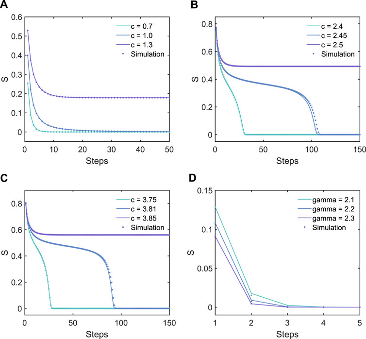
FIGURE 3. Theoretical results (solid lines) and numerical simulation results (dots) for k-core decompositions on multiplex networks with identical parameters. All simulations are performed on networks with 107 vertices, except that in the simulations of c = 2.45 (B), c = 3.81 (C), and γ = 2.1 (D), the networks contain 5 × 10⁷ vertices. (A) Results of the (1,1)-core pruning process on three different two-layer uncorrelated ER networks. It should be noted that in this case, it shows a continuous phase transition. (B) Results of the (1,1,1)-core pruning process on three different three-layer uncorrelated ER networks. In this case, the networks exhibit a discontinuous phase transition. (C) Results of the (2,2)-core pruning process on three different two-layer uncorrelated ER networks. It should be noted that in this case, the networks exhibit a discontinuous phase transition, different from the case shown (A). (D) Results of the (2,2)-core pruning process on three different two-layer uncorrelated SF networks. In this case, the (2,2)-core does not exist for γ > 2.
Overall, in this paper, we derive a new variation of the Non-Backtracking Expansion Branch called the Multicolor Non-Backtracking Expansion Branch, specially designed to solve the k-core pruning process on multiplex networks. In a multiplex network, each layer of the network is assigned a unique color, and then, the Multicolor Non-Backtracking Expansion Branch is constructed as an infinite tree having the same local structural information as the given multiplex network, when observed by non-backtracking walkers. We find that with this representation, one can obtain the analytical results of the k-core pruning process on any given multiplex network, regardless whether the correlation exists or not. The theoretical results obtained by our method are further validated by numerical simulations. Due to the diversity of edges in multiplex networks, the types of interactions that can be expressed will be much richer than those in a single-layer network. Many characteristic behaviors lacking in single-layer networks emerge in multilayer networks. For example, the phase transition of the k-core in a multi-layer network shows a different behavior compared to that of a single-layer network, as shown in Figure 3, and our method can be used for both single-layer and multi-layer networks and can obtain the analytical results of its k-core. Our method opens new possibilities to analytically solve the k-core pruning process on any given multiplex network, which is valuable for both theoretical studies and real-world applications.
The original contributions presented in the study are included in the article/Supplementary Material; further inquiries can be directed to the corresponding author.
G-YS designed the research; R-JW and G-YS performed the theoretical analysis; Y-XK, G-YS, and Y-CZ designed the figures and performed the numerical experiments. All authors wrote the manuscript.
The authors declare that the research was conducted in the absence of any commercial or financial relationships that could be construed as a potential conflict of interest.
All claims expressed in this article are solely those of the authors and do not necessarily represent those of their affiliated organizations, or those of the publisher, the editors, and the reviewers. Any product that may be evaluated in this article, or claim that may be made by its manufacturer, is not guaranteed or endorsed by the publisher.
1. Du N, Wu B, Pei X, Wang B, Xu L. Community detection in large-scale social networks. In: Proceedings of the 9th WebKDD and 1st SNA-KDD 2007 workshop on Web mining and social network analysis (ACM) (2007). p. 16–25.
2. Fortunato S. Community detection in graphs. Phys Rep (2010) 486:75–174. doi:10.1016/j.physrep.2009.11.002
3. Papadopoulos S, Kompatsiaris Y, Vakali A, Spyridonos P. Community detection in social media. Data Min Knowl Discov (2012) 24:515–54. doi:10.1007/s10618-011-0224-z
4. Weng L, Menczer F, Ahn YY. Virality prediction and community structure in social networks. Sci Rep (2013) 3:2522. doi:10.1038/srep02522
5. Kong YX, Shi GY, Wu RJ, Zhang YC. k-core: Theories and applications. Phys Rep (2019) 832:1–32. doi:10.1016/j.physrep.2019.10.004
6. Shang F, Chen B, Expert P, Lü L, Yang A, Stanley HE, et al. Local dominance unveils clusters in networks (2022). arXiv preprint arXiv:2209.15497.
7. Kitsak M, Gallos LK, Havlin S, Liljeros F, Muchnik L, Stanley HE, et al. Identification of influential spreaders in complex networks. Nat Phys (2010) 6:888–93. doi:10.1038/nphys1746
8. Li R, Wang W, Di Z. Effects of human dynamics on epidemic spreading in côte d’ivoire. Physica A: Stat Mech its Appl (2017) 467:30–40. doi:10.1016/j.physa.2016.09.059
9. Alvarez-Hamelin JI, Dall’Asta L, Barrat A, Vespignani A. Large scale networks fingerprinting and visualization using the k-core decomposition. In: Advances in neural information processing systems (2006). p. 41–50.
10. Serrano MÁ, Boguná M, Vespignani A. Extracting the multiscale backbone of complex weighted networks. Proc Natl Acad Sci U S A (2009) 106:6483–8. doi:10.1073/pnas.0808904106
11. Goltsev AV, Dorogovtsev SN, Mendes JFF. k-core (bootstrap) percolation on complex networks: Critical phenomena and nonlocal effects. Phys Rev E (2006) 73:056101. doi:10.1103/physreve.73.056101
12. Dorogovtsev SN, Goltsev AV, Mendes JFF. K-core organization of complex networks. Phys Rev Lett (2006) 96:040601. doi:10.1103/physrevlett.96.040601
13. Altaf-Ul-Amin M, Shinbo Y, Mihara K, Kurokawa K, Kanaya S. Development and implementation of an algorithm for detection of protein complexes in large interaction networks. BMC bioinformatics (2006) 7:207. doi:10.1186/1471-2105-7-207
14. Li X, Wu M, Kwoh CK, Ng SK. Computational approaches for detecting protein complexes from protein interaction networks: A survey. BMC genomics (2010) 11:S3. doi:10.1186/1471-2164-11-s1-s3
15. Antiqueira L, Oliveira ON, da Fontoura Costa L, Nunes Md. GV. A complex network approach to text summarization. Inf Sci (2009) 179:584–99. doi:10.1016/j.ins.2008.10.032
16. Fernholz D, Ramachandran V. Cores and connectivity in sparse random graphs. Austin, TX, USA: The University of Texas at Austin, Department of Computer Sciences (2004). technical report TR-04-13.
17. Schwarz J, Liu AJ, Chayes L. The onset of jamming as the sudden emergence of an infinite k-core cluster. Europhys Lett (2006) 73:560–6. doi:10.1209/epl/i2005-10421-7
18. Baxter G, Dorogovtsev S, Lee KE, Mendes J, Goltsev A. Critical dynamics of thek-core pruning process. Phys Rev X (2015) 5:031017. doi:10.1103/physrevx.5.031017
19. Wu RJ, Kong YX, Di Z, Zhang YC, Shi GY. Analytical solution to the k-core pruning process. Physica A: Stat Mech its Appl (2022) 2022:128260. doi:10.1016/j.physa.2022.128260
20. Boccaletti S, Bianconi G, Criado R, Del Genio CI, Gómez-Gardenes J, Romance M, et al. The structure and dynamics of multilayer networks. Phys Rep (2014) 544:1–122. doi:10.1016/j.physrep.2014.07.001
21. Szell M, Lambiotte R, Thurner S. Multirelational organization of large-scale social networks in an online world. Proc Natl Acad Sci U S A (2010) 107:13636–41. doi:10.1073/pnas.1004008107
22. Li R, Tang M, Hui P. Epidemic spreading on multi-relational networks. Acta Phys Sin (2013) 62:168903. doi:10.7498/aps.62.168903
23. Azimi-Tafreshi N, Gómez-Gardenes J, Dorogovtsev S. k−corepercolation on multiplex networks. Phys Rev E (2014) 90:032816. doi:10.1103/physreve.90.032816
24. Osat S, Radicchi F, Papadopoulos F. k-core structure of real multiplex networks. Phys Rev Res (2020) 2:023176. doi:10.1103/physrevresearch.2.023176
25. Radicchi F, Bianconi G. Redundant interdependencies boost the robustness of multiplex networks. Phys Rev X (2017) 7:011013. doi:10.1103/physrevx.7.011013
We use mathematical induction to prove the theorem. It is obvious that the theorem holds for n = 1. Now, we prove that if the theorem is true for n−1, the theorem can be established for n.
First, we prove the sufficiency, that is, for every 1 ≤ l ≤ R, when at least kl MNEBs in SMNEB(V) belong to Y[l],n−1, there must be V ∈ Sn. Since for every 1 ≤ l ≤ R, Y[l],n−1 ⊂ Y[l],n−2, we obtain V ∈ Sn−1, and in any given layer (for instance, the ith layer), suppose that
Next, we prove the necessity. We attempt to prove that when there exists an l in [1, R], which satisfies that at most kl−1 MNEBs in SMNEB(V) belong to Y[l],n−1, there must be V∉Sn. Since for an MNEB B(e[l],r, Vr) whose root is colored with cl in SMNEB(V) that does not belong to Y[l],n−1, from Theorem 1, we know that in SMNEB(e[l],r, Vr), either at most kl−2 MNEBs belong to Y[l],n−2, or there exists h ≠ l, 1 ≤ h ≤ R that at most kh−1 MNEBs belong to Y[h],n−2. Therefore, in SMNEB(Vr), there exists 1 ≤ h ≤ R that at most kh−1 MNEBs belong to Y[h],n−2. From the induction hypothesis, we know that Vr∉Sn−1, which means after (n−1)th pruning, in the lth layer, at most kl−1 neighbors of V survived. So either V has been pruned in (n−1)th pruning or even before, or it survived in the (n−1)th pruning but would be deleted in the nth pruning since its remaining neighbors in the lth layer are less than kl after the (n−1)th pruning; then, we have V∉Sn.
At this point, sufficiency and necessity are proved, and Theorem 2 can be established.
Figure A1 are B(e[1],(1,3), 3), B(e[1],(1,2), 2), B(e[2],(1,2), 2), B(e[2],(1,5), 5), and B(e[2],(1,8), 8), respectively. For k = (2, 1) core decomposition, we can find B(e[1],(1,3), 3) ∈ Y[1],∞, B(e[1],(1,2), 2) ∈ Y[1],∞, B(e[2],(1,2), 2) ∈ Y[2],∞, B(e[2],(1,5), 5) ∈ Y[2],∞, and B(e[2],(1,8), 8)∉Y[2],1. So in SMNEB(1), there are two MNEBs that belong to Y[1],∞ and two MNEBs that belong to Y[2],∞. So we have the vertex 1 ∈ S∞. For k = (2, 2), we can find that B(e[1],(1,3), 3) ∈ Y[1],2, but it does not belong to Y[1],3. B(e[1],(1,2), 2) ∈ Y[1],3, but it does not belong to Y[1],4. B(e[2],(1,2), 2) ∈ Y[2],3, but it does not belong to Y[2],4. B(e[2],(1,5), 5) ∈ Y[2],1, but it does not belong to Y[1],2. B(e[2],(1,8), 8)∉Y[2],1. So we can conclude that vertex 1 survives in the first two steps but will be deleted in the third pruning step.
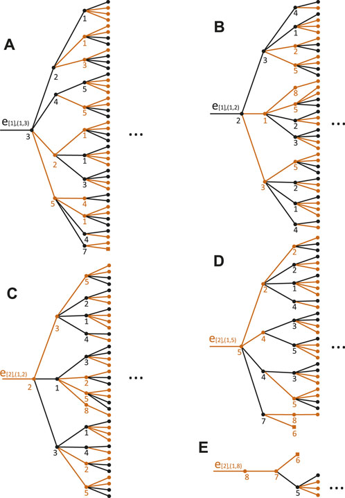
FIGURE A1. All five MNEBs in SMNEB(1) of the network shown in Figure 1. (A–E) represent the MBEB of e[1],(1,3), e[1],(1,2), e[2],(1,2), e[2],(1,5), e[1],(1,8), respectively.
Keywords: complex network, complex system, k-core, multiplex network, network theory
Citation: Wu R-J, Kong Y-X, Zhang Y-C and Shi G-Y (2022) Analytical results of the k-core pruning process on multiplex networks. Front. Phys. 10:1076314. doi: 10.3389/fphy.2022.1076314
Received: 21 October 2022; Accepted: 25 November 2022;
Published: 14 December 2022.
Edited by:
Xiyun Zhang, Jinan University, ChinaReviewed by:
Ruiqi Li, Beijing University of Chemical Technology, ChinaCopyright © 2022 Wu, Kong, Zhang and Shi. This is an open-access article distributed under the terms of the Creative Commons Attribution License (CC BY). The use, distribution or reproduction in other forums is permitted, provided the original author(s) and the copyright owner(s) are credited and that the original publication in this journal is cited, in accordance with accepted academic practice. No use, distribution or reproduction is permitted which does not comply with these terms.
*Correspondence: Gui-Yuan Shi, c2d5QGJudS5lZHUuY24=
Disclaimer: All claims expressed in this article are solely those of the authors and do not necessarily represent those of their affiliated organizations, or those of the publisher, the editors and the reviewers. Any product that may be evaluated in this article or claim that may be made by its manufacturer is not guaranteed or endorsed by the publisher.
Research integrity at Frontiers
Learn more about the work of our research integrity team to safeguard the quality of each article we publish.