 Huai-Yu Wang
95% of researchers rate our articles as excellent or good
Learn more about the work of our research integrity team to safeguard the quality of each article we publish.
Find out more
ORIGINAL RESEARCH article
Front. Phys. , 08 December 2022
Sec. Atomic and Molecular Physics
Volume 10 - 2022 | https://doi.org/10.3389/fphy.2022.1059968
This article is part of the Research Topic Quantum and Semiclassical Trajectories: Development and Applications View all 11 articles
Heisenberg guessed, after he established the matrix quantum mechanics, that the non-commutativity of the matrices of position and momentum implied that the position and momentum of a particle could not be precisely simultaneously determined. He consequently conjectured that time and energy should also have a similar relationship. Soon after, Robertson derived an inequality concerning the space coordinate and momentum, which was thought to be the mathematical expression of the uncertainty relation guessed by Heisenberg. Since then, people have tried various devices to prove the correctness of these two relations. However, no one conducted a careful analysis of Heisenberg’s primary paper. In this work, we point out some serious problems in Heisenberg’s paper and the literature talking about the uncertainty relationships: the physical concepts involved in the uncertainty relations are not clear; one physical concept had more than one explanation, i.e., switching concepts; there has never been measurement experiment to support the relations. The conclusions are that the so-called coordinate–momentum uncertainty relation has never been related to actual measurement and there does not exist a time–energy uncertainty relation.
As soon as Heisenberg founded quantum mechanics (QM) in matrix form [1–3], he acutely perceived that the matrices of the position and momentum of a particle were non-commutative. He thought that this non-commutativity should have some physical meaning. In a later paper [4], he guessed that the physical meaning of the non-commutativity was that the position and momentum of a microscopic particle could not be precisely simultaneously determined by experimental measurement. He was unable to provide an explicit expression for that, but merely presented qualitative discussion, including the gedanken experiments. He inferred consequently that there was a similar relationship between time and energy.
Soon after that, Robertson [5] derived an inequality, which was believed the mathematical expression of the uncertainty relation guessed by Heisenberg. Thus, the guess of the uncertainty relationship proposed by Heisenberg was generally accepted by people, and this was set in stone. Almost all QM textbooks introduce the coordinate–momentum relation and time–energy relation [6–30]. The uncertainty relations are thought of as fundamental ones in QM. They have been frequently mentioned by researchers and were even promoted as a principle—uncertainty principle [6–12].
When the present author carefully read the introductions and explanations of the uncertainty relations in Heisenberg’s primary paper [4] and the literature, questions emerged. A striking problem is that the uncertainty relations ought to be related to actual measurement, but it seems not to be so. Even in [4], Heisenberg merely talked about idealized experiments. The narrations connecting the uncertainty relations and the experiments are farfetched and specious. Confusions between different conceptions appear frequently. As a matter of fact, someone has been aware that there exist wrong explanations in the literature [31, 32]. We think that it is desirable to analyze in detail all the aspects involved in the uncertainty relations.
In the 1920s, Heisenberg, Schrödinger, Dirac et al. performed pioneering work in founding QM, which was a completely new field in physics. A series of new concepts merged. Some new concepts were formed. Among the new concepts, some were not very clear to people; they were not very clear even to these pioneers themselves, which should not be surprising. Hence, no one could guarantee that their works were flawless.
For example, when Schrödinger proposed his wave equation of QM, he unknowingly put down the negative kinetic energy (NKE) Schrödinger equation (33). However, this NKE Schrödinger equation was never realized by himself and others and was abandoned since then. We found that the NKE Schrödinger equation could be obtained by taking low-momentum approximation from relativistic quantum mechanics equations (RQMEs), and it was of explicit physical meanings [34, 35]. Dirac explained the NKE solutions of his RQME as representing antiparticles. Although people know that this explanation implied contradictions, no one could propose the right scenario to resolve the contradictions. We have given a correct explanation of the NKE solutions [35, 36].
There are two reasons that make people not aware of these pioneers’ mistakes in some aspects. One is that due to their genius achievements, people think that what they said was right. The other is that the related mistakes have not brought perceivable affection up till now. For instance, if there is no so-called uncertainty relationship, the evaluations and measurements in QM are not affected. The new theories raised after the uncertainty relations had been established, such as RQMEs, quantum electrodynamics (QED), quantum field theory (QFT), and quantum information, did not resort to the uncertainty relations. The computation of the band structures in solid-state materials and of nuclear physics does not need uncertainty relations. Physical experiments have never been arranged under the guidance of uncertainty relations, in spite of that, they are called principles. The uncertainty relations are usually employed to provide explanatory notes to some known phenomena and results.
After almost one hundred years, as later generations, we have grasped knowledge much more and wider than the pioneers did. People nowadays ought to have more sophisticated and rigorous reasoning. We should be able to recognize what the problems left by these pioneers are and how to resolve them. With clearer distinguishing and understanding of physical concepts, we are able to solve some difficulties left in QM [34–42].
The study of physics obeys physical laws. The physical laws are represented by fundamental equations and statements. The conclusions in physics need to be verified by experiments, which means that quantitative results are necessary. Theoretically, quantitative results are obtained by mathematical derivation starting from the fundamental equations. Theoretical discussions observe rigorous logical reasoning. We believe that in order to avoid the flaws in physical discussions as far as possible, some principles related to the physical contents discussed should be obeyed besides the mathematical derivation. The principles are presently called the basic viewpoints of the author.
The basic viewpoints depended on the concrete contents under discussion. The author’s previous papers [34–42] concerned some basic problems in QM. When we discussed one of these problems, certain viewpoints were based on [35, 42].
The uncertainty relationship is believed to be a fundamental topic in QM. In the present work, we are going to investigate this topic based on certain points of view. In the author’s following work, more topics will be touched on, and corresponding basic viewpoints will be stemmed on.
All the basic viewpoints we have been aware of are listed in Supplementary Appendix SA. We think that only when these viewpoints are abided by can one guarantee logical rigorousness and validity of the conclusions in discussing physical problems. Or, conception confusion may occur, and subsequently, the problem may not be solved correctly.
Here we mention one of the basic points of view. In QM, we always deal with wave functions. Every wave function satisfies a fundamental QM equation. Explicitly, the fundamental QM equation is in the form of
Here, the coordinate variables are not explicitly shown. In this paper, we always assume that (Eq. 1.1) is Schrödinger equation. If the Hamiltonian H is time-independent, the dependence of the wave function on time can be written as
Thus, the function
Every wave function is necessarily the solution of Eq. 1.1. The wave functions of stationary states observe Eq. 1.3. In other words, when one discusses a wave function, he must be able to put down the corresponding Hamiltonian H. This is important. In textbooks, some functions are treated as wave functions because of their seemingly good behaviors. However, they are not the solutions of Eq. 1.1, i.e., there is no corresponding Hamiltonian. In Section 2, we will see two examples: the wave packet and wave train with the finite length for moving particles.
In Sections 2 and 3, we discuss coordinate–momentum and time–energy uncertainty relations, respectively. We will point out that physical conceptions are confused in the literature in discussing the two uncertainty relations. In [4], Heisenberg proposed the possible relations between the uncertainties of position and momentum, directed against single particles. Naturally, the similar relation between time and energy that he guessed was also for single particles. We stress this because in the literature, the problems of single-particles are confused with those of many-body systems. Section 4 is further discussion, and Section 5 contains the conclusions. Supplementary Appendix SA lists our basic viewpoints. Supplementary Appendix SB introduces the derivation of the so-called coordinate–momentum uncertainty relation.
There are confusions of concepts when the coordinate–momentum uncertainty relation is discussed. The inequality derived by Robertson [5] was irrespective of experiments and Heisenberg’s primary paper [4]. This section presents a detailed analysis.
In this paper, we always consider the case of one dimension.
The paper [4] was the first one to talk about possible uncertainty relationships. The whole article did only qualitative discussion with no rigorous mathematical derivation. Heisenberg, based on his established QM in matrix form, found that the commutator of the two matrices q and p had the following result:
The nonzero result meant that the two matrices could not exchange the order in their product. From this, he guessed that when a particle’s position and momentum were measured, both had some uncertainties.
“Let
Here, the definition of the uncertainty of q was obvious: “
According to the basic viewpoint I.1 in Supplementary Appendix SA, every physical concept should have an explicit mathematical expression, or people would not clearly understand the conception.
First, in QM, a particle is described by its wave function. The wave function is the function of the spatial coordinate q, that is to say, q is an argument in a function, e.g., Eqs. 3, 12–(14) in [4]. In Heisenberg’s words, “Let
Next, we discuss the contents in the QM field. Following the viewpoint II.2, a wave function must be the solution of a fundamental QM equation. Heisenberg put down functions for discussion, but some of them were not the solutions of the Schrödinger equation for the system under consideration.
“If, for any definite state variable
This should be a wave function in QM. Such a function was called a Gaussian wave packet and used in the literature [6, 13–16]. It is time independent. Only the stationary eigenfunctions of a harmonic oscillator are of the form of
It is seen that the function (Eq. 2.3) is not a free particle. We do not know what a potential
We are unable to write down a
In Eq. 2.3, q is the spatial coordinate of the wave function, but not the position of the electron. Heisenberg confused the concepts.
Eq. 18 in [4] was
This was a time-dependent function. When it is substituted into the left-hand side of Eq. 1.1, the result is
We are unable to find a time-dependent Hamiltonian
Therefore Eq. 2.6 is not a wave function in QM.
For the wave function (22) in [4], one was unable to write a corresponding Hamiltonian as well, and so it was not a wave function in QM.
When writing down a function, one should first prove that it is the solution of a fundamental QM equation or has its corresponding Hamiltonian. Otherwise, it cannot be treated as a wave function in QM.
Third, Heisenberg did not present explicit expressions or rigorous mathematical derivations when he mentioned some physical conceptions.
For example, he mentioned “statistical error” more than once, but we do not know what he meant by it.
In Eq. 2.6, a concept of “radiation damping” was used. However, Heisenberg did not provide the mathematical derivation for the form in Eq. 2.6. In QM, a single particle does not have the concept of “radiation damping.” This concept must belong to a many-body system.
In [4], the argument below Eq. 8 was questionable. A beam of electrons was arranged to run through two fields successively in two different manners. In the second manner, no derivation was presented. Therefore, one could not know how the result
Fourth, according to viewpoint I.3, when a gedanken experiment leads to a positive conclusion, it cannot explain anything. Such a conclusion could neither be proved nor be disproved.
In short, Heisenberg’s primary paper [4] lacked rigorous mathematics, was not quantitatively related to real experiments, and was not very clear in some physical concepts.
Heisenberg’s paper [4] just considered the measurement precisions of the position and the momentum of a single particle.
In 1929, Robertson [5] derived the famous mathematical inequality, see Supplementary Appendix SB. The conclusion was that the mean square errors of coordinate and momentum obeyed the following inequality:
This inequality was believed to be the mathematical expression of the uncertainties of coordinate and momentum that Heisenberg guessed. So, (2.9) was called the Heisenberg uncertainty relation.
Here, we distinguish the concepts of the position of a particle and coordinate. Heisenberg discussed the uncertainties of the measured position and momentum of a particle, so that his assumed relation was called the position–momentum uncertainty relation. However, in QM, a particle at a state is described by a wave function, which is a function of coordinates. The
According to the current understanding, the
Now, we explain that it is not right to understand the
Usually, the recognition of (2.9) is that if one measures the position x and momentum p of a particle, they cannot be precisely simultaneously measured, and the smaller the measuring deviation of one quantity is, the greater the other. This recognition is incorrect.
Since (2.9) is regarded as the relation between the ncertainties of position and momentum, it ought to be related to the statistics of measured quantities. This prompts us to explain the implication of the inequality and the way of statistics of measured quantities.
The coordinate is expressed by x, and the momentum operator is
The inner product of any two functions ψ and φ is defined by
We perform the following calculations:
The four calculated quantities meet (2.9).
Because the forms of 2.11–2.14 seem the same as that of the definition of mean square error, people mistakenly believe that 2.11–2.14 are of the meanings of the mean square error in the sense of measurement.
When talking about 2.9, people usually think that the smaller the one of
For a one-dimensional harmonic oscillator, the nth stationary state wave function is denoted by
We turn to look at the comparison between the ground states of different systems. A hydrogen atom and an atomic nucleus have different dimensions. Compared with the hydrogen atom, the dimension of the nucleus is smaller, and so, the uncertainty
Personally, Eq. 2.9 has only one usage: it can be used to judge if the wave function solved from (1.1) has some error. If the
People usually say that (2.9) concerns measurement, and it shows that the position and momentum of a particle cannot be precisely simultaneously measured. We recall how the statistics of the measured results are made.
Suppose that there is a sample, Y. We measure its value. The ith measured value is denoted as yi. After N times of the measurement, this sample’s averaged value and mean square deviation are evaluated by
and
Now, we have a QM system, and a mechanical quantity F is to be measured. Suppose that an appropriate device is designed, and the value of F can be measured experimentally.
According to QM, the average of the mechanical quantity F in a state ψ is
The inner product is defined by (2.10). In order to evaluate the average (2.17), in principle, at any spatial coordinate x, the value of F should be measured. Actually, one has to check, if possible, the measurement at discrete x points. Hence, the integration is replaced with the form of summation
The coefficients
In this way, the mean square deviation
However, what is the meaning of
In QM, the state of a particle is represented by its wave function. The wave function distributes in space at any time. One cannot say that the wave function is at a point at one instant and another point at the next instant. The physical quantity F belongs to the whole QM system and is not fixed to discrete spatial points.
We do not know how to experimentally measure
Furthermore, from Eq. 2.9 itself, we are unable to see the concepts of “position uncertainty” and “momentum uncertainty”, since it is irrespective to measurement. That is to say, the uncertainty relation (2.9) itself does not contain the concepts of “position uncertainty” and “momentum uncertainty”, since it does not contain the information related to measurement.
The relation (2.9) is sometimes called a principle. However, no one designs an experiment based on this so-called principle.
The conclusion is that Eq. 2.9 is irrespective to measurement.
We have pointed out above that in [4], there was no rigorous argument and mathematical derivation, and some concepts were confused. However, people a priori believed that the content in this paper was right and the mathematical expression was what Robertson [5] provided. Some textbooks presented (2.9) without explanation [8, 17, 18]. Some others tried various devices in order to explain that this uncertainty relation was correct.
Because the narration in [4] was not clear, when later people talked about the uncertainty relation, they did not have fixed rules, but depended on their own imaginative development. Different people had different explanations. Each explanation was unable to overturn others. Therefore, according to the basic viewpoint I.2, none of the explanations were right. The so-called examples, that were believed to support the uncertainty relation, were just farfetched ex-post explanations.
There are three typical examples giving farfetched explanations: finite-length wave train or a piece of truncated plane wave, single-slit diffraction, and the ground state of hydrogen atom. Before analyzing these examples, we distinguish between two concepts: a particle’s dimension and the uncertainty of its position.
A particle’s dimension and the uncertainty of its position are two different conceptions.
In QM, a particle at a state is described by a wave function. For each wave function, we are able to roughly define a range in space, outside which the wave function can be regarded as zero. This range is defined as the dimension of this particle at this state. For instance, in an infinitely deep square potential with width a, the dimension of a particle is just the potential width a. For a one-dimensional harmonic oscillator, the ground state wave function is
The De Broglie relation tells us that as long as a particle’s momentum is known, its dimension can be roughly estimated by
Here, we regard De Broglie wave length as the particle’s dimension. The De Broglie relation tells us that the larger the momentum of a particle, the less its dimension. It is seen that Eq. 2.2 guessed by Heisenberg was more like the De Broglie relation.
The uncertainty of a particle’s position can be roughly defined as the precision, or error range, of the measured position of the particle.
We stress that a particle’s dimension and the uncertainty of a particle’s position are two different concepts. The former is uniquely determined by the wave function, independent of measurement, whereas the latter depends on the measurement devices and measurement process.
For example, Heisenberg mentioned [4] that when a photon was employed to collide with a particle, “the highest attainable accuracy in the measurement of position is governed by the wavelength of the light.” Thus, roughly speaking, when the light wavelength is λ, the measuring precision of the particle’s position is λ; when the light wavelength is 2λ, the precision will be 2λ.
In literature, the two concepts were confused frequently.
In [4], Heisenberg put down a wave packet, Eq. 2.3, and said that the wave function “differs appreciably from zero only in a region of spread
The confusion of the two concepts, or concept stealing, also occurred later [14, 19].
Figures 1A,B are often used to represent the two states of a moving particle. This picture is utilized to explain the coordinate–momentum uncertainty relation [9]. An intuitive understanding is that the shorter the particle’s dimension or its position uncertainty, the greater its momentum uncertainty. Comparison of Figures 1A,B prompted such a recognition: “we can see very clearly that the better the position is defined, the more poorly is the momentum defined” [9].
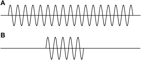
FIGURE 1. Two wave trains (interrupted sine waves) with finite lengths. (A) Longer length. (B) Shorter length.
Here, we are considering a particle with a mass. Figure 1 represents the wave functions of the particle. Following basic viewpoint II.2, the wave functions should be the solutions of Eq. 1.1.
The two pictures in Figure 1 are actually the stationary wave functions in two one-dimensional infinitely deep square potential wells with different widths. Because the widths are different, the two wells are of different Hamiltonians. The two wave functions are in different systems. Comparing the positions and momenta of the particles in the different systems is meaningless. Furthermore, the average of momentum in each state is exactly zero. In this case, discussing the momentum uncertainty is meaningless.
It can be certain that a particle which is marching is not represented by the functions in Figure 1. Thus, the two pictures in Figure 1 are not wave functions in QM for describing a moving particle.
Now, suppose that
First, we should not say that the uncertainty of
Next, since
Another analysis commonly used is to write a function’s Fourier transformation and inverse Fourier transformation [9].
It was analyzed that the more localized the
Equations 2.21 and 2.22 are Fourier transformation and its inverse of each other. This is a general mathematic property, not a unique property in QM. Furthermore, the localization and extension of the
Single-slit experiment is often used to explain the uncertainty relation of a particle [9, 13, 14].
Let the width of a slit be d and the wavelength of particles be λ. The particles go through the slit and diffraction occurs as
This is not correct. When a particle is within the slit, its wave function is zero outside of the slit. At this moment, the width d is the dimension of the particle, which is independent of measurement. However,
If the measurement precisions of the position and momentum of a particle obey the uncertainty relation, these precisions ought to be obtained in experimental measurements. In single-slit diffraction experiment, neither a single particle’s position nor its momentum is measured. The energy of the incident particle is already known. Since the slit width d is known, the diffraction pattern, the distribution of the outgoing particles with diffraction angle, is determined, which can be evaluated by means of the diffraction law before the experiment. The diffraction pattern obtained experimentally is in agreement with the theoretical calculation, and is stable. The single-slit diffraction experiment just lets particles go through a slit, and all the information is known before the experiment. According to viewpoint I.3, this experiment is not a measurement.
The single-slit experiment is just an observation of a phenomenon, not a measuring manipulation. Every wave, when going through a region, the room of which is less than the wave length, yields diffraction. Water waves are the same, and no one would explain the water diffraction by uncertainty relation. The behavior of water waves is explained by the Huygens–Fresnel principle. The wavelength of radio waves can be as long as kilometers, so that they can diffract in a larger room. The distribution of the electromagnetic field can be evaluated by Maxwell equations under specific boundary conditions. These diffractions are irrespective to uncertainty relation.
Suppose that there are two slits, with widths
In [4], Heisenberg considered using photons to probe electrons, a measurement of single particle. In the single-slit experiment, no physical quantity of a single particle is measured. The single-slit diffraction shows the angular distribution of a large number of particles after going through the slit. The distribution is stable, and there is no concept of uncertainty.
Single-slit diffraction is a collective effect of many particles. Trying to explain the uncertainty relation by the single-slit diffraction is a confusion of the single-particle system and many-particle system.
Figure 2.8 in [19] actually showed the distribution of a large number of particles, and not the uncertainty of a particle’s position.
There is a way of estimating the energy of the ground state of a hydrogen atom [6, 9, 20, 21], which is thought of as an application of the uncertainty relation. The energy of a hydrogen atom reads
The dimension of this system is very small, i.e., the r is very small and
is used to express
By taking the derivative of
In this course, it seems that the uncertainty relation (2.25) is employed. This method is also employed to estimate the ground state energy of a nucleus.
First, this example is irrespective to measurement. It is just an estimation of the energy minimum. Second, the above procedure can be simplified. Using
We stress once more that a particle’s dimension is a definite quantity, whereas its position’s uncertainty relies on measurement.
Until now, when discussing the uncertainty relation, often idealized experiments have been concerned, which are irrelative to the experiment of measurement.
Actually, there is no such experiment in which the position and momentum of a particle are measured simultaneously, and their uncertainties are estimated from the measured information, so as to meet Eq. 2.9.
To gain the uncertainty of a particle’s position, one first has to measure its position. Nevertheless, in QM, a particle is described by a wave function, and has a dimension as having been defined in Section 2.3.1. In QM, the concept of a particle’s position is not clearly defined. Because of this fact, in experiments, no measurement of the so-called position of a particle is carried out.
People did measure a particle’s momentum, and estimate the uncertainty from the information of the experiment. However, they did not measure the particle’s position in the same experiment simultaneously. There are two examples [14].
One is that the momentum of a charged particle is measured by deflection in a constant magnetic field, the strength of which is denoted by B. An electron with a charge e enters the magnet after passing through a diaphragm with width
At the instant at which the electron enters the magnet through the first diaphragm, it moves along the y axis. The uncertainty is estimated as
Thus, it seems that
However, the right-hand side of Eq. 2.29 has been already known before the measurement. In the experiment, the position of the electron is not detected, and consequently, one is unable to estimate the precision of the position of the electron from measurement. This experiment does not need the knowledge of QM.
Another experiment measuring a particle’s momentum is to let a photon collide with the particle. Before the collision, the photon’s frequency
Assuming that the uncertainty at the time of the collision is
Within the time, the particle can go a distance of
Substitution of (2.31) into (2.32) leads to the uncertainty of the position of the particle.
It seems that
This explanation is problematic. The relation 2.31 has neither rigorous mathematical derivation nor experimental verification. Eq. 2.32 assumes that within the time uncertainty
The common features of these two examples are as follows: the measurement of a particle’s position is out of question; the measured particles are actually treated as classical ones. Though the momentum is measured, the estimated
In Ref. [4], having discussed the possible uncertainty relation between the position and momentum, Heisenberg noticed that the product of the coordinate and momentum was of the dimension of angular momentum, and the result was proportional to the Planck constant. He associated the commutator of time and energy, and thus postulated the following commutator:
Then, imitating the discussion of position and momentum, he thought that the uncertainties of time and energy obeyed, similarly to (2.2), the relation
Later, people accepted his postulation. Furthermore, imitating
Since
Eq. 3.3 is the so-called time–energy uncertainty, but it is even worse than the coordinate–momentum uncertainty relation.
Heisenberg put forth Eq. 3.1 without any derivation and proof. He did not even present the concrete form of the operator E. Hilgevoord [32] thought that “a relation like” (3.1) “does not occur in quantum mechanics”. His reason was that “there is no Poisson bracket defined between t and H. Consequently, in quantum mechanics, one does not have a relation like” Eq. 3.3. “Accordingly, there is no natural analog for energy and time of the ‘canonical’ uncertainty relations” Eq. 2.9.
At the time when QM was established, Heisenberg himself did not know explicitly what the relation between time and energy was. The mathematical theory of QM had not been accomplished yet. In Heisenberg’s paper [4], there was neither rigorous derivation nor an association with real experiments.
Thus, Heisenberg did not give a convincing conclusion, but people deemed that what he said was right. Later, many people tried to show that there was indeed the inequality (3.3). Everyone raised his own version, without rigorous derivation and experimental correspondence.
Until 1961, “there has been an erroneous interpretation of uncertainty relations of energy and time.” [31] Until 1990, “no general agreement has been reached. One finds physicists claiming that ‘there is no energy–time uncertainty relation at all,’ while others stress, for instance, that the relation is applied quite effectively to the analysis of individual short-lived elementary particles (resonances). Even among those who accept the validity of the relation, there is appreciable disagreement as to meanings of the relation.” [43] Until 1996, “It is generally thought desirable that quantum theory entail an uncertainty relation for time and energy similar to the one for position and momentum. Nevertheless, the existence of such a relation has still remained problematic” [32].
As a matter of fact, up to now, there has been no final verdict with respect to the time–energy uncertainty relation.
It should also be noted that Heisenberg discussed the measurement of individual particles, which can be inferred from his examples about the uncertainty relation (2.9). Subsequently, the discussion of time–energy uncertainty should be for individual particles. However, later, people often discuss many-particle systems.
Now we start to carefully analyze the so-called time–energy uncertainty relation.
First, let the two operators in Eq. (B1) be time and energy, respectively,
does not have a definite result. When the Hamiltonian H is independent of time, the result is zero.
The key is that the coordinate and momentum operators on the left-hand side of (2.1) have explicit forms, no matter what function they act on. By contrast, the form of Hamiltonian H depends on the system under investigation. Hilgevoord noticed that “for a system of particles, one should not demand a communication relation between t and H as a complement to the ones between q and p, nor could there be such a commutation relation.” [32].
Time t is not an operator. According to Pauli, “the introduction of an operator t is basically forbidden, and the time t must necessarily be considered as an ordinary number (‘c-number’).” [12] The average of t in any normalized state is still the time itself,
Therefore, there is no way to derive a time–energy uncertainty relation starting from (3.4) in the way in Supplementary Appendix SB.
People may think that although the Hamiltonian H in (3.4) depends on systems, the operator
It seems, then, that imitating the procedure of deriving (2.9) can lead to (3.3). It is not so. Obviously, the averages of time t and its square
The conclusion is that there is no way to acquire (3.3) through the procedure in Supplementary Appendix SB. In [44], Eq. 3.3 was just a hypothesis.
Here we intend to clarify the implication of the operator
Following this definition, (3.1) could be understood as (3.5), but this problematic.
When we put down
An operator should have its eigenvalues and corresponding eigenfunctions under appropriate boundary conditions, such as a momentum operator. The operator
Then, why do people think of
It is stressed that
When these two points are met, the result calculated through
is of the meaning of the energy average in this state.
For any function of
Since the implication of the operator
Let Hamiltonian H be independent of time and its eigenfunction be denoted as
We construct a wave function
This result shows that for any
We explain how this difficulty is yielded. When taking the Taylor expansion of the factor
instead of the right-hand side of (3.10). If
is still an eigenfunction of the H, it must meet (1.1).
Since
The right-hand side of (3.11) and (3.14) should be equal. It is seen that
In [4], the relation (3.3) between the uncertainties of time and energy was guessed without derivation, and the discussion was vague. People believed that what Heisenberg said was right. Some first assumed (3.3), resembling (3.3), and then, tried to derive it by supposing various scenarios. Different persons present the derivation based on their own understanding of the uncertainties of time and energy. Among different derivations, none of them could overturn the others. Therefore, according to viewpoint I.2, none was correct. In fact, every derivation was apparently right but actually wrong. Although it was noticed [31, 32] that some of the derivations were wrong, a thorough analysis is desired.
In the following, we list several derivations and present our comments. In each case, we extract the concepts of
Before the introduction, we emphasize that in inequality (B14),
and
It is a definite quantity determined by the known wave function but not a variable. One more point should be stressed that
1) Using the concept of wave packet [14, 15, 19]:
This is for a single particle. Suppose that the particle is a wave packet with width
On the other hand, the wave packet has some extension in momentum space, so that the particle’s energy has an uncertainty
The product of these two equations yields
Then Eq. 2.9 is used to result in (3.3), “which limits the product of the spread
Comment:
Since the right-hand side of (3.19) is just (2.9), the
The use of (3.19) means that Eqs. (2.9) and (3.3) ought to be compatible. However, the two relations were thought to express two different and incompatible viewpoints in [19].
Here,
2) Making use of the formulas in Supplementary Appendix SB [3, 14, 19, 21, 23]:
When a quantity A varies, the time it needs to change
We make use of the formula
Then, by (3.15)
The combination of these three equations results in
Comment:
We point out that Eq. 3.20 is strange. In the denominate and following equations, A is regarded as an operator, and the numerator should be written as
In Eq. 3.20, the
The authors of [45] recast (3.22) to be the form
Here, the
3) Making use of the difference of two energy levels [3, 14]:
Suppose that a particle had two energy levels,
When the two states superpose, the particle oscillates between the two states and the oscillation period is
Then,
which is explained as the time–energy uncertainty relation.
Comment:
Here, the τ is the oscillation period between two energies of the system, and the
Eq. 3.26 is simply the copy of (3.25), but the concepts are endowed different connotations, i.e., concept stealing. In Eq. 3.26, the
4) Using the concept of “time packet” [6]:
It was assumed that a particle’s behavior was a pulse or ‘time packet’.
“We consider the case such that
where the function
As the
Since
the width of the distribution in energy,
In this way, it seems that the uncertainty relation can be proved.
Comment:
Here, the
It is well known that a light pulse can be produced experimentally. But what about a massive particle? This imagined pulse or ‘time packet’ of a massive particle is not possible. No one is able to find a Hamiltonian H such that the solution
5) Making use of the interaction between the measured system and measuring device [10, 24, 46]:
The measured system and measuring device are combined to become a larger system. In other words, the whole system is divided into two parts, measured system and measuring devices, the energies of which are E and ε, respectively. “We suppose that it is known that at some instant these parts have definite values of the energy, which we denote by E and ε, respectively.” “The energies E, ε, on the other hand, can be measured to any degree of accuracy at any instant” [10].
Because of the interaction between the two parts, each time the measurement would cause the energy E to change, say, to be
According to this formula, “The most probable value of
This was called the “uncertainty relation for energy.”
Comment:
According to this result, the energy conservation in QM was understood in an alternative way. “It shows that, in quantum mechanics, the law of conservation of energy can be verified by the means of two measurements only to an accuracy of the order of
It was believed that the relation
This scenario is totally different from the above ones. Here the energy of a system can be measured in any accuracy, which contradicts the uncertainty of energy.
According to [10, 46], because the measured system is interacted by the measuring device, its energy shifts after the measurement. The amount of the shift and the time interval between adjacent measurements form the time–energy uncertainty relation: “the smaller the time interval
In the transition probability formula, the difference of two energy levels is used, which is not the energy uncertainty. Furthermore, in [10], Eq. (42.3) was valid under a condition of (42.1) which required that the frequency ω should not be zero. It is hard to understand the transition expressed by (3.32) without releasing or absorbing photons.
Equations (3.32) and (3.33) contradict each other. Eq. 3.32 means that there were two energy levels
Here, the
This scenario was criticized in [31].
In [10, 46], following the above content, momentum variation was discussed by collision as an example. Nevertheless, Eq. 3.32 was obtained by perturbation theory, while collision could not be treated by the perturbation theory.
The last part of Section 44 in [10] related the difference
All in all, it is seen from the entries 1) – 5) that people presumed the relation (3.3) and then designed certain ideas to scrape it together. None of the above scenarios were connected to a real measurement. All of them are incorrect.
Different people had different explanations of the
In [13], the relation (3.3) was given without derivation. The explanation was that “an energy determination that has an accuracy
In [14], the
In [19], there were contradictory statements. One was that “the energy of a system can be determined with arbitrary precision at any time.” The other was that Eq. 3.3, written as
In [24], the
One explanation of the
In Eq. 3.3, the
In a wave function, there is a factor containing energy E and time t,
then
The wave function decays with time exponentially. After a time period of about
the wave function almost disappears. Due to this fact, we say that the lifetime of this state is about
Here, we emphasize the following points: (1) The lifetime τ of a state is determined by the imaginary part, not the real part, of the state’s energy. (2) The lifetime is defined by (3.36). It is not the case that we have first the two quantities
In a many-particle system, there are interactions between particles, such as electron–phonon interaction, collision, and so on. Due to the interactions, elementary excitations are formed, and they are of finite lifetimes. An elementary excitation’s lifetime is determined by the imaginary part of its energy [47, 48].
A detailed analysis was given in [25]. The interactions inside a system result in transitions between energy levels. The transitions in turn cause an energy shift and broadening. Now we introduce the analysis.
Suppose that in a system there are two states denoted by a and b, respectively. When there is no interaction, both are stationary states, and their energies are
The change yields not only a shift of the energy but also an imaginary part of the energy, the latter being determined by transition probability. This imaginary part determines the lifetime of the state
It is seen that in about time
the state
Meanwhile, the energy of the final state b has a broadening with a Lorentz line shape, the half height width of which happens to be Γ, too. We denote this half height width by
Then,
Equations (3.39) and (3.41) seem to be the form of the time–energy uncertainty relation, but they are not. The former is the definition of the
People subjectively thought that what Heisenberg said in his paper [4] were certainly right, and the inequality that Robertson derived [5] was just what Heisenberg wanted to express. Under these presumptions, people tried their best to present explanations to the coordinate–momentum uncertainty relation, and to derive the so-called time–energy uncertainty relation. There is no uniform and standard explanation. Several scenarios were proposed. From the source, the discussions in Heisenberg’s primary paper [4] were ambiguous. The explanations and derivations are of the following defects.
One mathematical symbol has different explanations, that is, concept stealing. In the coordinate–momentum uncertainty relation, the
A truncated plane wave with finite length for a moving particle is not the wave functions in QM.
All the derivations of the so-called time–energy uncertainty relation are not rigorous, but simply patchwork. The last words in [31], “energy can be measured reproducibly in an arbitrarily short time”, utterly negated the so-called time–energy uncertainty relation.
No real measurement was touched. Gedanken experiments were assumed, which could not verify the uncertainty relations. The application of the coordinate–momentum uncertainty relation was just to make some ex-post explanations to well-known phenomena such as single-slit diffraction. Even in these explanations there were confusions of the concepts.
In discussion of the time–energy uncertainty relation, the problems in one-particle and many-particle systems were confused.
There is more than one explanation for an uncertainty relation. This fact itself illustrates that none of the explanations is right. If one explanation was right, the other would be no longer displayed.
We have mentioned in Introduction the reasons that people do not realize the problem of the uncertainty relations. The uncertainty relations have never been related to real measurements, and solving problems and establishing new theories in QM do not resort to the uncertainty relations.
Up to now, the quantum measurement problem, that what precisely happens when a quantum measurement is performed, is still in dispute [49, 50], but the so-called uncertainty principle for quantum measurement was proposed long before. That is strange!
Heisenberg’s primary paper did not explicitly present an uncertainty relation.
Robertson derived the coordinate–momentum uncertainty relation
There is no definite result for the commutation of time and Hamiltonian
The original contributions presented in the study are included in the article/Supplementary Material; further inquiries can be directed to the corresponding author.
H-YW carried out the whole work of this article.
This work was supported by the National Natural Science Foundation of China (Grant no. 12234013).
The author declares that the research was conducted in the absence of any commercial or financial relationships that could be construed as a potential conflict of interest.
All claims expressed in this article are solely those of the authors and do not necessarily represent those of their affiliated organizations, or those of the publisher, the editors, and the reviewers. Any product that may be evaluated in this article, or claim that may be made by its manufacturer, is not guaranteed or endorsed by the publisher.
The Supplementary Material for this article can be found online at: https://www.frontiersin.org/articles/10.3389/fphy.2022.1059968/full#supplementary-material
1. Heisenberg W. Quantum-theoretical Re-interpretation of kinetic and mechanical relations. Z Phys (1925) 333: 879-893. In: Van Waerden BL, editor. Source of quantum mechanics, New York: Dover Publications Inc. (1968). p. 261–276.
2 Aitchison I. J. R., MacManus D. A., Snyder T. M. Understanding Heisenberg’s “magical” paper of july 1925: A new look at the calculational details. Am J Phys (2004) 72:1370–9. doi:10.1119/1.1775243
3 Razavy M. Heisenberg’s quantum mechanics. London, UK: World Scientific Publishing Co. Pte. Ltd. (2011).
4 Heisenberg W. Uber den anschaulichen Inhalt der quantentheoretischen Kinematik und Mechanik. Zeitschrift fur Physik (1927) 43: 172-198. “The Physical Content of Quantum Kinetics and Mechanics”. In: Wheeler JA, Zurek WH, Editor. Quantum Theory and Measurement. Princeton: Princeton University Press (1983). 62-84.
6 Bransden B. H., Joachain C. J. Quantum mechanics. 2nd ed. London, UK: Pearson Education Limited (2000).
7 Bes D. R. Quantum mechanics A modern and concise introductory course. Berlin, Germany: Spinger-Verlag (2004).
10 Landau L. D., Lifshitz F. M. Quantum Mechanics, Oxford, UK: Pergamon Press (1977). p. 2, 47, 157.
11 Weinberg S. Lectures on quantum mechanics. 2nd ed. Cambridge, UK: Cambridge University Press (2015).
12 Pauli W. General principles of quantum mechanics. Berlin, Germany: Springer-Verlag (1980). p. 63.
16 Band Y. B., Avishai Y. Quantum Mechanics with Application to Nanotechnology and Information Science. Amsterdam: Elsivier Ltd (2013). p. 68, 297.
17 Bohm A. Quantum mechanics: Foundations and applications. 3rd ed. New York, NY, USA: Springer-Verlag (1993).
18 Zettili N. Quantum mechanics: Concepts and applications. New York, NY, USA: John Wiley & Sons (2001). p. 28.
19 Auletta G., Fortunato M., Parisi G. Quantum Mechanics. Cambridge, UK: Cambridge University Press (2009). p. 82–89, 130–40.
21 Ballentine L. E. Quantum Mechanics A Modern Development. 2nd ed., Singapore: World Scientific Publishing Co. Pte. Ltd. (2015). p. 223-227, 271, 345.
23 Kroemer H. Quantum mechanics for engineering, materials science, and applied physics. Englewood Cliffs, NJ, USA: Prentice-Hall (1994). p. 249–50.
26 Beck M. Quantum mechanics theory and experiment. New York, NY, USA: Oxford University Press (2012).
28 Peres A. Quantum theory: Concepts and methods. New York, NY, USA: Kluwer Academic Publishers (2002).
29 Cohen-Tannoudji G., Diu B., Laloë F. Quantum Mechanics, 1. New York, NY, USA: John Wiley & Sons (1977). p. 250.
31 Ahronov Y., Bohm D. Time in the quantum theory and the uncertainty relation for time and energy. Phys Rev (1961) 122:1649–58. doi:10.1103/PhysRev.122.1649
32 Hilgevoord J. The uncertainty principle for energy and time. Am J Phys (1996) 64:1451–6. doi:10.1119/1.18410
33 Schrödinger E. Ann Phys (1926). 386 (18): 109–139.; Quantisation as a problem of proper values (Part IV). In: Collected papers on wave mechanics. London and Glasgow: Blackie & son Limited (1926). p. 102–123.
34 Wang H. Y. New results by low momentum approximation from relativistic quantum mechanics equations and suggestion of experiments. J Phys Commun (2020) 4:125004. doi:10.1088/2399-6528/abd00b
35 Wang H. Y. The modified fundamental equations of quantum mechanics. Phys Essays (2022) 35(2):152–64. doi:10.4006/0836-1398-35.2.152
36 Wang H. Y. Fundamental formalism of statistical mechanics and thermodynamics of negative kinetic energy systems. J Phys Commun (2021) 5:055012. doi:10.1088/2399-6528/abfe71
38 Wang H. Y. Macromechanics and two-body problems. J Phys Commun (2021) 5:055018. doi:10.1088/2399-6528/ac016b
39 Wang H. Y., Virial theorem and its symmetry. J. North China Inst Sci Technology (2021) 18(4):1–10. (in Chinese).
40 Wang H. Y. Resolving problems of one-dimensional potential barriers based on Dirac equation. J North China Inst Sci Technology (2022) 19(1):97–107. (in Chinese) doi:10.19956/j.cnki.ncist.2022.01.016
41 Wang H. Y. Evaluation of cross section of elastic scattering for non-relativistic and relativistic particles by means of fundamental scattering formulas. astp (2022) 16(3):131–63. doi:10.12988/astp.2022.91866
42 Wang H. Y. There is no vacuum zero-point energy in our universe for massive particles within the scope of relativistic quantum mechanics. Phys Essays (2022) 35(3):270–5. doi:10.4006/0836-1398-35.3.270
43 Busch P. On the energy-time uncertainty relation, Part I: Dynamical time and time indeterminacy. Found Phys (1990) 20(1):1–32. doi:10.1007/BF00732932
44 Busch P. On the energy-time uncertainty relation. Part II: Pragmatic time versus energy indeterminacy. Found Phys (1990) 20(1):33–43. doi:10.1007/BF00732933
45 Mandelstam L., Tamm I. The uncertainty relation between energy and time in nonrelativistic quantum mechanics. J Phys (Ussr) (1945) 9:249–54.
46 Landau L., Peierls R. Erweiterung des Unbestimmtheisprinzips fur die relativistische Quantentheorie. Z Phys (1931) 69: 56; translated into English: Lev Davidovich Landau and Rudolf Peierls, Extension of the uncertainty principle to relativistic quantum theory in Quantum Theory and Measurement. edited by John Archibald Wheeler and Wojciech Hubert Zurek. Princeton: Princeton University Press (1983). 465-472.
48 Wang H. Y. Green’s function in condensed matter physics. Beijing: Alpha Science International ltd. and Science Press (2012).
49 Mermin N. D. There is no quantum measurement problem. Phys Today (2022) 76(6):62–3. doi:10.1063/PT.3.5027
Keywords: coordinate–momentum uncertainty relation, time–energy uncertainty relation, measurement, dimension of a wave function in quantum mechanics, uncertainty, lifetime of energy level
Citation: Wang H-Y (2022) Exploring the implications of the uncertainty relationships in quantum mechanics. Front. Phys. 10:1059968. doi: 10.3389/fphy.2022.1059968
Received: 02 October 2022; Accepted: 04 November 2022;
Published: 08 December 2022.
Edited by:
Yujun Zheng, Shandong University, ChinaCopyright © 2022 Wang. This is an open-access article distributed under the terms of the Creative Commons Attribution License (CC BY). The use, distribution or reproduction in other forums is permitted, provided the original author(s) and the copyright owner(s) are credited and that the original publication in this journal is cited, in accordance with accepted academic practice. No use, distribution or reproduction is permitted which does not comply with these terms.
*Correspondence: Huai-Yu Wang, d2FuZ2h1YWl5dUBtYWlsLnRzaW5naHVhLmVkdS5jbg==
Disclaimer: All claims expressed in this article are solely those of the authors and do not necessarily represent those of their affiliated organizations, or those of the publisher, the editors and the reviewers. Any product that may be evaluated in this article or claim that may be made by its manufacturer is not guaranteed or endorsed by the publisher.
Research integrity at Frontiers
Learn more about the work of our research integrity team to safeguard the quality of each article we publish.