 Pablo Giuliani
 Kyle Godbey
 Edgard Bonilla
 Frederi Viens2,4*
 Jorge Piekarewicz
- 1FRIB/NSCL Laboratory, Michigan State University, East Lansing, MI, United States
- 2Department of Statistics and Probability, Michigan State University, East Lansing, MI, United States
- 3Department of Physics, Stanford University, Stanford, CA, United States
- 4Rice University, Department of Statistics, Houston, TX, United States
- 5Department of Physics, Florida State University, Tallahassee, FL, United States
A covariant energy density functional is calibrated using a principled Bayesian statistical framework informed by experimental binding energies and charge radii of several magic and semi-magic nuclei. The Bayesian sampling required for the calibration is enabled by the emulation of the high-fidelity model through the implementation of a reduced basis method (RBM)—a set of dimensionality reduction techniques that can speed up demanding calculations involving partial differential equations by several orders of magnitude. The RBM emulator we build—using only 100 evaluations of the high-fidelity model—is able to accurately reproduce the model calculations in tens of milliseconds on a personal computer, an increase in speed of nearly a factor of 3,300 when compared to the original solver. Besides the analysis of the posterior distribution of parameters, we present model calculations for masses and radii with properly estimated uncertainties. We also analyze the model correlation between the slope of the symmetry energy L and the neutron skin of 48Ca and 208Pb. The straightforward implementation and outstanding performance of the RBM makes it an ideal tool for assisting the nuclear theory community in providing reliable estimates with properly quantified uncertainties of physical observables. Such uncertainty quantification tools will become essential given the expected abundance of data from the recently inaugurated and future experimental and observational facilities.
1 Introduction
Nuclear science is undergoing a transformational change enabled by the commissioning of new experimental and observational facilities as well as dramatic advances in high-performance computing [1]. The newly operational Facility for Rare Isotope Beams (FRIB), together with other state-of-the-art facilities throughout the world, will produce short-lived isotopes that provide vital information on the creation of the heavy elements in the cosmos. In turn, earth and space-based telescopes operating across the entire electromagnetic spectrum will constrain the nuclear dynamics in regimes inaccessible in terrestrial laboratories. Finally, improved and future gravitational-wave detectors will provide valuable insights into the production sites of the heavy elements as well as on the properties of ultra-dense matter at both low and finite temperatures [2–9].
To fully capitalize on the upcoming discoveries, a strong synergy will need to be further developed between theory, experiment, and observation. First, theory is needed to decode the wealth of information contained in the new experimental and observational data. Second, new measurements drive new theoretical advances which, in turn, uncover new questions that motivate new experiments. From the theoretical perspective, sophisticated and highly-accurate ab initio methods have been developed to solve the complicated many-body problem. Besides the adoption of a many-body solver, one needs to specify a nuclear interaction that is informed by two- and three-nucleon data. A highly successful approach relies on a nuclear interaction rooted in chiral effective field theory (EFT). Chiral EFT—a theoretical framework inspired by the underlying symmetries of QCD—provides a systematic and improvable expansion in terms of a suitable small parameter, defined as the ratio of the length scale of interest to the length scale of the underlying dynamics [10–12]. During the last decade, enormous progress has been made in our understanding of the equation of state (EOS) of pure neutron matter by systematically improving the chiral expansion [13–19]. However, the chiral expansion breaks down once the relevant energy scale of the problem becomes comparable to the hard scale associated with the underlying dynamics. This fact alone precludes the use of chiral perturbation theory in the study of high density matter.
A more phenomenological approach that could be extended to higher densities is Density Functional Theory (DFT). Developed in quantum chemistry [20] but now widely used in nuclear physics, DFT is a powerful technique whose greatest virtue is shifting the focus away from the complicated many-body wave function that depends on the spatial coordinates of all particles, to an energy density functional (EDF) that depends only on the three spatial coordinates of the ground state density. Moreover, DFT guarantees that both the exact ground-state density and energy of the complicated many-body system may be obtained from minimizing a suitable functional [21, 22]. In an effort to simplify the solution of the problem, the Kohn–Sham formalism reformulates the DFT problem in favor of one-particle orbitals that may be obtained by solving self-consistently a set of equations that closely resemble the structure of the well-known Hartree equations [22]. It is important to note that the theorems behind DFT offer no guidance on how to construct the correct EDF. This fact is mitigated in nuclear physics by incorporating as many physical insights as possible into the construction of the functional, and then calibrating the parameters of the model by using the available experimental and observational data. However, unlike chiral EFT, DFT is unable to quantify systematic errors associated with missing terms in the functional that may become important at higher densities. Nevertheless, given that modern covariant EDFs are informed by the existence of two-solar mass neutron stars, the parameters of the model encode (at least partially) information on the high-density component of the EOS.
The calibrated models are not static, however, and theory must be nimble in its response to the exciting new data that will emerge from future experiments and observations. In the particular case of DFT, new data must be promptly incorporated into the refinement of the EDF to explore the full impact of the new information. This is particularly relevant given that nuclear physics has the ability to predict the structure and properties of matter in regions inaccessible to either experiment or observation. For example, one may use Bayesian inference to identify strong correlations between a desired property, which cannot be measured, and a surrogate observable that may be determined experimentally. However, Bayesian methods often require multiple evaluations of the same set of observables for many different realizations of the model parameters. If the nuclear observables informing the EDF are computationally expensive, then direct Bayesian inference is highly impractical. This computational challenge has motivated many of the recent efforts by the nuclear theory community in the development and adoption of emulators to accelerate computation speed with a minimal precision loss [23–35]. In this work we explore the application of one such class of emulators, the Reduced Basis Method (RBM) [36–38], which falls under the umbrella of the general Reduced Order Models (ROM) techniques [39, 40].
The Reduced Basis Method encapsulates a set of dimensionality reduction approaches that generally aim at speeding up computations by approximating the solution to differential equations with just a handful of active components (the reduced basis). These methods have been shown to exhibit speed increases of several orders of magnitude in various areas of science and engineering [41–44], including specific applications for uncertainty quantification [45, 46], and have been recently demonstrated to be viable for applications in nuclear physics DFT [29]. Solving the full system of differential equations self-consistently in the framework of covariant DFT is not a particularly demanding computational task for modern computers, usually taking around a minute for a heavy nucleus such as 208Pb. The computational bottleneck appears when millions of such evaluations must be carried out sequentially to perform Bayesian inference, and the problem multiplies when several nuclei are involved or if one wants to consider and compare different EDFs. A speed-up factor of three orders of magnitude or more provided by techniques such as the RBM could bridge the computational gap and enable new scientific advancements that would otherwise be impossibly or significantly more expensive. The adoption of these methods, paired together with leadership-class computing infrastructure, will enable the quick response that is needed to take full advantage of the vast wealth of experimental and observational data that will be coming in the next years.
The intent of this manuscript is to develop and showcase a pipeline for the calibration and uncertainty quantification of a nuclear model—a covariant energy density functional—enabled by the RBM emulation. To that goal, in Sec. II we provide a brief introduction to the relativistic mean field model we use, culminating with the set of differential equations that need to be solved in order to calculate nuclear observables. In Sec. III we present the reduced basis methodology, alongside an explanation on how it is used to construct an emulator that simplifies the computations of the DFT model. In Sec. IV we explain the theory and implementation of the Bayesian statistical analysis used to calibrate the model parameters, with full uncertainty quantification. In Sec. V we present and discuss the results of the calibration, displaying the Bayesian posterior distribution of the model parameters, together with the model predictions with quantified uncertainties for binding energies and charge radii, as well as the correlation between the slope of the symmetry energy L and the neutron skin thickness of both 208Pb and 48Ca. These two observables have been the focus of recent experimental campaigns [47–49], and its widespread implications are of great interest to the nuclear physics and astrophysics communities [50, 51]. Finally, in Sec. VI we present our conclusions and outlooks, with a perspective on the role that this class of emulators could play, in the near future, on the nuclear theory-experiment cycle enhanced by statistics and machine learning [31, 52, 53].
2 Relativistic mean field calculations
The cornerstone of covariant density functional theory is a Lagrangian density that includes nucleons and mesons as the effective degrees of freedom. Besides the photon that mediates the long-range Coulomb interaction, the model includes the isoscalar-scalar σ meson, the isoscalar-vector ω meson, and the isovector-vector ρ meson [54, 55]. The interacting Lagrangian density consists of a nucleon-nucleon interaction mediated by the various mesons alongside non-linear meson interactions [55–60]. That is,
The first line in the above expression includes Yukawa couplings gs, gv, and gρ of the isoscalar-scalar (ϕ), isoscalar-vector (Vμ), and isovector-vector (bμ) meson fields to the appropriate bilinear combination of nucleon fields. In turn, the second line includes non-linear meson interactions that serve to simulate the complicated many-body dynamics and that are required to improve the predictive power of the model [56–58]. In particular, the two isoscalar parameters κ and λ were designed to soften the equation of state of symmetric nuclear matter at saturation density. In turn, the isoscalar parameter ζ also softens the EOS of symmetric nuclear matter but at much higher densities. Finally, the mixed isoscalar-isovector parameter ∧v was introduced to modify the density dependence of the symmetry energy, particularly it slope at saturation density. For a detailed account on the physics underlying each terms in the Lagrangian see Refs. [60, 61].
2.1 Meson field equations
In the mean-field limit, both the meson-field operators and their corresponding sources are replaced by their ground state expectation values. For spherically symmetric systems, all meson fields and the photon satisfy Klein-Gordon equations of the following form [59]:
Where we have defined Φ = gsϕ, Wμ = gvVμ, and Bμ = gρbμ. The various meson masses, which are inversely proportional to the effective range of the corresponding meson-mediated interaction, are given by ms, mv, and mρ. The source terms for the Klein-Gordon equations are ground-state densities with the correct Lorentz and isospin structure. Finally, the above scalar (s) and vector (v) densities are written in terms of the occupied proton and neutron Dirac orbitals:
Here t identifies the nucleon species (or isospin) and n denotes the principal quantum number. We note that some of the semi-magic nuclei that will be used to calibrate the energy density functional may have open protons or neutron shells. In such case, we continue to assume spherical symmetry, but introduce a fractional occupancy for the valence shell. For example, in the particular case of 116Sn, only two neutrons occupy the valence d3/2 orbital, so the filling fraction is set to 1/2.
2.2 Dirac equations
In turn, the nucleons satisfy a Dirac equation with scalar and time-like vector potentials generated by the meson fields. The eigenstates of the Dirac equation for the spherically symmetric ground state assumed here may be classified according to a generalized angular momentum κ. The orbital angular momentum l and total angular momentum j are obtained from κ as follows:
where κ takes all integer values different from zero. For example, κ = − 1 corresponds to the s1/2 orbital. The single-particle solutions of the Dirac equation may then be written as
where m is the magnetic quantum number and the spin-spherical harmonics
Where the upper numbers correspond to protons and the lower ones to neutrons, and we have used the shorthand notation a = {nκt} to denote the relevant quantum numbers. The mass of both nucleons is denoted by M, and it is fixed to the value 939 MeV. Finally, ga(r) and fa(r) satisfy the following normalization condition:
Looking back at Eq. 3, we observe that the proton and neutron vector densities are conserved, namely, their corresponding integrals yield the number of protons Z and the number of neutrons N, respectively. In contrast, the scalar density is not conserved.
2.3 Ground state properties
From the solution of both the Klein-Gordon equations for the mesons Eq. 2 and the Dirac equation for the nucleons Eq. 6, we can calculate all ground-state properties of a nucleus composed of Z protons and N neutrons. The proton and neutron mean square radii are determined directly in terms of their respective vector densities:
Following [60] we approximate the charge radius of the nucleus by folding the finite size of the proton rp as:
where we have used for the radius of a single proton rp = 0.84 fm [62].
In turn, the total binding energy per nucleon E/A− M, includes contributions from both the nucleon and meson fields: E = Enuc + Emesons. The nucleon contribution is calculated directly in terms of the single particle energies obtained from the solution of the Dirac equation. That is,
where the sum is over all occupied single particle orbitals, Ea is the energy of the ath orbital, and (2ja + 1) is the maximum occupancy of such orbital. For partially filled shells, one must multiply the above expression by the corresponding filling fraction, which in the case of 116Sn, is equal to one for all orbitals except for the valence d3/2 neutron orbital where the filling fraction is 1/2.
The contribution to the energy from the meson fields and the photon may be written as
where the above expression includes individual contributions from the σ, ω, and ρ mesons, the photon, and the mixed ωρ term. In terms of the various meson fields and the ground-state nucleon densities, the above contributions are given by.
Following [60], in this work we calibrate the relativistic mean field model by comparing the calculations of charge radii and binding energies with the experimentally measured values for the doubly magic and semi-magic nuclei: 16O, 40Ca, 48Ca, 68Ni1, 90Zr, 100Sn, 116Sn, 132Sn, 144Sm, 208Pb.
2.4 Bulk properties parametrization
The Lagrangian density of Eq. 1 is defined in terms of seven coupling constants. These seven parameters plus the mass of the σ meson define the entire 8-dimensional parameter space (the masses of the two vector mesons are fixed at their respective experimental values of mv = 782.5 MeV and mρ = 763 MeV). Although historically the masses of the two vector mesons have been fixed at their experimental value to simplify the search over a complicated parameter landscape, such a requirement is no longer necessary. Bayesian inference supplemented by RBMs can easily handle two additional model parameters. Given that the aim of this contribution is to compare our results against those obtained with the traditional fitting protocol, we fix the masses of the two vector mesons to their experimental values, and defer the most ambitious calibration to a future work.
Once the theoretical model and the set of physical observables informing the calibration have been specified, one proceeds to sample the space of model parameters: α ≡ {ms, gs, gv, gρ, κ, λ, ∧v, ζ}. However, given that the connection between the model parameters and our physical intuition is tenuous at best, the sampling algorithm can end up wandering aimlessly through the parameter space. The problem is further exacerbated in covariant DFT by the fact that the coupling constants are particularly large. Indeed, one of the hallmarks of the covariant framework is the presence of strong—and cancelling—scalar and vector potentials. So, if the scalar coupling gs is modified without a compensating modification to the vector coupling gv, it is likely that no bound states will be found. To overcome this situation one should make correlated changes in the model parameters. Such correlated changes can be implemented by taking advantage of the fact that some of the model parameters can be expressed in terms of a few bulk properties of infinite nuclear matter [60, 64]. Thus, rather than sampling the model parameters α, we sample the equivalent bulk parameters θ = {ms, ρ0, ϵ0, M*, K, J, L, ζ}. In this expression, ρ0, ϵ0, M*, and K are the saturation density, the binding energy, effective nucleon mass, and incompressibility coefficient of symmetric nuclear matter evaluated at saturation density. In turn, J and L are the value and slope of the symmetry energy also at saturation density. The quartic vector coupling ζ is left as a “bulk” parameter as the properties of infinite nuclear matter at saturation density are largely insensitive to the value of ζ [57]. The virtue of such a transformation is twofold: first, most of the bulk parameters given in θ are already known within a fairly narrow range, making the incorporation of Bayesian priors easier and natural, and second, a modification to the bulk parameters involves a correlated change in several of the model parameters, thereby facilitating the success of the calibration procedure.
In the context of density functional theory, Eqs 2–6 represent the effective Kohn–Sham equations for the nuclear many-body problem. Once the Lagrangian parameters α have been calculated from the chosen bulk parameters θ, these set of non-linear coupled equations must be solved self-consistently. That is, the single-particle orbitals satisfying the Dirac equation are generated from the various meson fields which, in turn, satisfy Klein-Gordon equations with the appropriate ground-state densities as the source terms. This demands an iterative procedure in which mean-field potentials of the Wood-Saxon form are initially provided to solve the Dirac equation for the occupied nucleon orbitals which are then combined to generate the appropriate densities for the meson field. The Klein-Gordon equations are then solved with the resulting meson fields providing a refinement to the initial mean-field potentials. This procedure continues until self-consistency is achieved, namely, the iterative process has converged.
In the next section we show how the reduced basis method bypasses such a complex and time-consuming procedure by constructing suitable reduced bases for the solution of both the Klein-Gordon and Dirac equations.
3 The reduced basis method
A system of coupled differential equations in the one-dimensional variable r, such as Eq. 2 and Eq. 6, can be computationally solved by numerical methods such as finite element or Runge-Kutta. We shall refer to the numerical solutions obtained from those computations as high fidelity solutions for the rest of the discussion. Those approaches possess an intrinsic resolution Δr—such as the grid spacing in the case of finite element or the step size in the case of Runge-Kutta2. For a given interval L in which we are interested in solving the equations, each of the functions involved will have roughly
In turn, once the differential operators such as
Both the traditional Runge-Kutta solver and the finite element solver we developed to iteratively tackle Eqs 2 and 6 have L = 20 fm, Δr = 0.05 fm, and therefore
The RBM implementation we construct in this work consists of two principal steps: “training and projecting” [29]. In the first step we build the RB using information from high fidelity solutions, while in the second step we create the necessary equations for finding the approximate solution by projecting over a well-chosen low-dimensional subspace. The following subsections explain both steps in detail.
3.1 Training
We begin by proposing the corresponding RB expansion for each function involved in Eqs 2 and 6:
The subscripts n and κ have been omitted from the gnκ and fnκ components for the sake of clarity, but it is important to note that the expansion will have unique coefficients ak, and possible different number of basis ng and nf for each level. The functions with sub-index k, Ak(r) for example, form the RB used to build their respective approximations,
Once chosen, each RB is fixed and will not change when finding approximated solutions to Eqs 2 and 6 for different parameters α. The coefficients
For future applications going beyond the spherical approximation it will be important to modify the approach accordingly, both in expanding the number of basis states to capture the richness of the solutions and in directly including information on the occupation of the single particle orbitals. This can be done at either the Hartree-Fock-Bogoliubov or the Hartree-Fock + BCS level and will naturally address the issue of level crossings and deformation at the expense of the slower performance associated with larger bases and more coupled equations to be solved. The trade-off is tempered by the fact that, because the RBM does not depend on the original dimensionality of the problem, moving from a spherical picture to full 3D will not be as heavily penalized as the high fidelity solver.
There are several approaches for the construction of the reduced basis [36, 37], most of which involve information obtained from high fidelity solutions for a sample of the parameters α. For this work, we choose the Proper Orthogonal Decomposition (POD) approach, which consists of building the RB as the first n components (singular vectors) of a Singular Value Decomposition (SVD) [65]—see also Principal Component Analysis (PCA) [66]—performed on a set of high fidelity solutions.
For each nucleus involved we compute high fidelity evaluations for 50 parameter sets sampled from the multivariate Gaussian distributions obtained in the calibration performed in [60]. We perform the SVD on each of the four fields and each of the wave functions for the respective protons and neutron levels for all ten nuclei considered in this study. For example, for 48Ca for protons and neutrons there are six and seven fa(r) and ga(r), respectively. Figure 1 shows the normalized singular values σk/σ1 for the field and nucleon wave functions for 48Ca and 208Pb. Each singular value represents how much of the total variance in the entire sample that particular component is capable of explain [40]. A fast exponential decay of the singular values can indicate that a RB with few components should be able to approximate the full solution with good accuracy (see also the discussion on the Kolmogorov N-width in Chapter V of [36]).
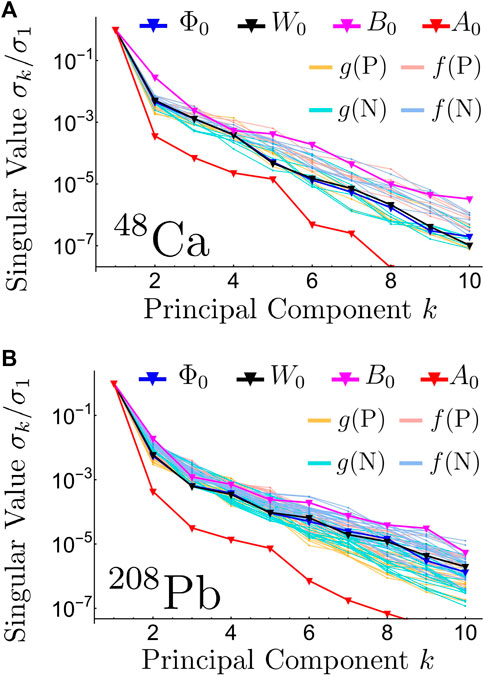
FIGURE 1. Normalized singular values σk/σ1 for the fields Φ0(r), W0(r), B0(r), and A0(r), and the single particle wave functions of the upper gnκ(r) and lower fnκ(r) components for 48Ca (A) and 208Pb (B). The single particle proton levels are denoted as g(P) and f(P) for the upper and lower components, respectively, while the single particle neutron levels are denoted as g(N) and f(N) for the upper and lower components, respectively. There are six proton levels and seven neutron levels for 48Ca (A), while for 208Pb there are sixteen proton levels and twenty-two neutron levels.
Figure 2 shows the first three principal components obtained from the SVD of the 50 high fidelity evaluations for the Φ0(r) and A0(r) fields, the upper component g(r) of the first neutron level, and the lower component f(r) for the last proton level for 48Ca. The figure also shows the corresponding 50 high fidelity solutions, although the spread is barely noticeable for the two wave function components, and is imperceptible outside of the inset plot for the photon field A0(r). We observed a similar small spread of the fields and wave functions for all the nuclei considered for the 50 high fidelity evaluations. This is consistent with the fact that the relativistic mean field model has been calibrated to reproduce ground state experimental observables such as masses and radii within a 0.5% error3 [60]. Appreciable variations of the solutions would deteriorate such values.
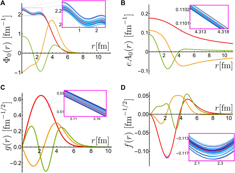
FIGURE 2. First three principal components in red, orange, and green respectively, for Φ0(r) (A), eA0(r) (B), the first g(r) for neutrons (C), and the sixth f(r) for protons (D) in 48Ca. The second and third components (in orange and green) have been re-scaled arbitrarily for plotting convenience. The 50 solutions used in the training set are shown in different shades of blue in each figure. The spread of such solutions is barely visible for Φ0(r) and f(r), and almost undetectable for the other two cases. The spread is further enhanced in the inset plots within the magenta squares in each sub figure.
Choosing how many reduced bases to include for each field or wave function—the upper limits on the sums in Eq. 14 [nΦ, nW, nB, nA, ng, nf]—is a non-trivial process. In general, the more basis used the more precise the approximation will be, but that comes at the trade-off of an increased calculation time. This choice will not depend only on the relative importance of the singular values shown in Figure 1, but rather on the quantities we are interested in calculating after solving the coupled differential equations. For example, for 48Ca, the photon field A0(r) has the fastest decaying singular values shown in Figure 1, which could indicate that we need a smaller basis to reproduce it to the same level of accuracy than any of the other fields, such as B0(r). Nevertheless, if our primary objective is to obtain accurate calculations for binding energies and charge radii, for example, it might be the case that we need to reproduce A0(r) to much better precision than B0(r), requiring nA > nB. We elaborate this discussion later when we describe our method for selecting the number of basis for each function.
3.2 Projecting
For a fixed nucleus and a chosen RB configuration we have nΦ + nW + nB + nA free coefficients for the fields,
For example, consider we are working with 48Ca which has six proton levels and seven neutron levels. If we set three RB for every field and wave function expansion in Eq. 14, we will have 12 coefficients associated with the fields, 36 coefficients and six energies associated with the protons, and 42 coefficients and seven energies associated with the neutrons. This amounts for a total of 103 unknown quantities that must be determined from 103 equations. Each single particle level for protons and neutrons has an associated normalization condition shown in Eq. 7. These normalization equations go in par with the unknown energies. The rest of the unknown coefficients—90 in this example—are determined from the Galerkin projection equations that we now describe. The Galerkin method [67] is the traditional approach for obtaining such coefficients in the RBM [37, 39].
Let us denote the set of field functions and wave functions in the compact notation Ξ≡{Φ0, W0, B0, A0, g, f} and their respective RB approximation
For example,
Finding a solution Ξ for given parameters α means finding a collection of fields and wave functions such that all the operators
Where we have made the choice of projecting each operator
Following our previous approach [29], we choose the “judges” to be the same as the RB expansion, as it is common practice with the Galerkin method [68]. For example, in the case of 48Ca with three basis for every field and wave function, since the photon field RB expansion
We also note that the dependence of Eqs 2 and 6 on the parameters α is affine, which means that every operator can be separated into a product of a function that only depends on α and a function that only depends on r. For example, the non-linear coupling between the isoscalar-vector meson ω and the isovector-vector meson ρ in Eq.2c reads:
For a concrete example, consider 48Ca now with only two basis for all functions. Each of the two projection equations associated with the proton’s g and f Eq. 16e and Eq. 16f contains a total of 22 terms. The equation for f for the first proton level—with the choice of basis we describe in the next section—with all numbers printed to two decimals precision reads:
3.3 Accuracy vs. speed: Basis selection
As with many other computational methods, the RBM posses a trade-off between accuracy and speed. If we use more bases for the expansions Eq. 14 we expect that our approximation will be closer to the high fidelity calculation, but that will come at the expense of more coefficients to solve for in the projection equations Eq. 16. If we use too few bases, the underlying physical model will be miss-represented when compared with experimental data, but if we use too many bases we might waste computational time to obtain an unnecessary accuracy level. To find a satisfactory balance we study the performance of the RBM, both in terms of accuracy and speed, for different basis size configurations on a validation set containing 50 new high fidelity evaluations drawn from the same distribution as the one we used for the training set [60].
As a metric of performance we define the emulator root mean squared errors as:
For the charge radius, and as:
For the total binding energy. In both expressions Nv is the total number of samples in the validation set (50) and the superscripts “mo” and “em” stand for the high fidelity model and the RBM emulator, respectively.
A straightforward approach for exploring different basis configurations consists of setting all basis numbers {nΦ, nW, nB, nA, ng, nf} to the same value n. There are two main disadvantages of this approach. First, the basis increments can be too big, making it harder to obtain a good trade-off. For example, in the case of 208Pb with n = 2 we have a total of 160 basis, while for n = 3 we jump straight to 240. Second, the accuracy in the emulation of the observables could be impacted differently by how well we reproduce each function involved in Eq. 2 and Eq. 6. Having a leverage that allows us to dedicate more resources (bases, that is) to more crucial functions could be therefore beneficial, and the simplistic approach with a common number n is unable to optimize the computational resources in that sense.
On the other hand, exploring all possible basis size configurations for a given maximum basis size is a combinatorial problem that can quickly become intractable. Therefore, we decided to follow a Greedy-type optimization procedure in which we incrementally add new basis to the current configuration, choosing the “best” local option at each step. The basis are chosen from the principal components obtained from the training set of 50 high fidelity runs. For all the nuclei the starting configuration was seven basis for each one of the fields {Φ0, W0, B0, A0} and two basis for each of the wave functions g and f on all the nucleus’ levels. On each step, we add one more basis to both g and f to the four levels across both protons and neutrons which were reproduced most poorly in the previous iteration on the validation set. The “worst performers” are chosen alternating in terms of either the single particle energies (serving as a proxy for the total binding energy), and the L2 norm on the wavefunctions themselves (serving as a proxy for the proton and neutron radius). The fields basis numbers are all increased by one once one of the wave functions basis number reaches their current level (7 in this case).
For example, for 48Ca we start with seven basis for the four fields {nΦ, nW, nB, nA} = {7, 7, 7, 7}, and {ng, nf} = {2, 2} for every one of the six levels for protons and seven levels for neutrons. On the first step we compare the RBM calculations with the 50 high fidelity solutions from the validation set and identify the first neutron level, and the first, third, and fifth proton levels as the worse (on average) estimated single particle energies. Consequently, their respective basis are increased by their third principal components (see Figure 2): {ng, nf} = {3, 3}. On the next step, we re-calculate the RBM solutions with the new updated basis and identify the fifth neutron level, and the second, third, and sixth proton levels as the worst performances in terms of the overall wave function sense (the L2 norm). This procedure is repeated as the overall basis number increases as is illustrated in Figure 3 for 48Ca and 208Pb. We observed similar behaviors for the other eight nuclei involved in this study.
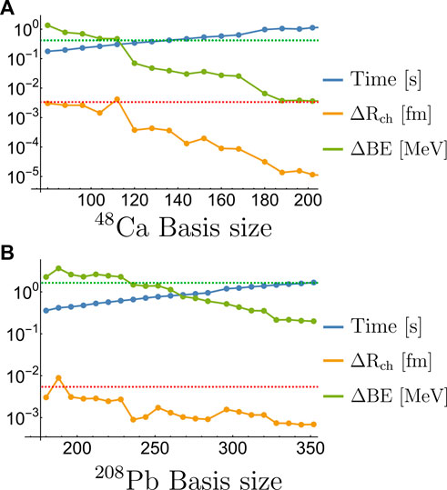
FIGURE 3. Performance of the RBM emulator for 48Ca (A) and 208Pb (B) as the total number of basis is increased following the Greedy algorithm described in the text. The dashed red and green lines in both plot indicate an error of 0.1% in the charge radius and total binding energy, respectively. The computation time per sample is calculated solving the RBM equations in Mathematica, which is substantially slower than the production emulator used in the calibration and detailed in Sec. IIID.
For the range of basis explored, the overall performance for both the charge radius and total binding energy roughly improves exponentially, although not monotonically5, with the total basis number. The error in the radius and binding energy reduces by more than a factor of 100 for 48Ca and by a factor of 10 for 208Pb. The computational time also increases exponentially, expanding almost an entire order of magnitude for both nuclei.
To select an optimal configuration of bases we used as a target a 0.1% error in both observables for all nuclei involved, which is roughly three times smaller than the average deviation between the originally calibrated RMF and the available experimental values [60]. These targets are shown as the red and green dashed lines in Figure 3. Table 1 shows the basis size for the chosen basis and the results from this validation analysis. In the case where we would like to have a faster emulator at the expense of accuracy, we could choose a smaller basis size from the configurations showed in Figure 3. In the case where we need a more accurate emulator for particular calculations, configurations with more basis functions could be chosen at the expense of speed.

TABLE 1. Results from the basis selection procedure using the 50 samples from the validation set.
3.4 RBM code optimization
The offline stage consisting of the symbolic construction of the Galerkin projection equations and the expressions for the observables of interest is performed in Mathematica, resulting in polynomial equations in the parameters and RB coefficients such as Eq. 18. These equations are then parsed and converted into both Python and Fortran functions which can then be compiled into a library and evaluated in the calibration driver software. The explicit Jacobian matrix is also constructed and parsed in the same way, resulting in fewer evaluations of the polynomial equations and thus faster convergence of the root finding routine. This automated pipeline from symbolic representation in Mathematica to compiled Python library vastly simplifies the development process of the emulator and allows for various basis sizes to be included at will while ensuring an efficient implementation.
For the Python implementation Cython is used to first convert the Python code into C which is subsequently compiled into a Python compatible library. The Fortran implementation is similarly compiled using the NumPy f2py tool to produce a performant Fortran library with an appropriate Python interface. Regardless of the generating code, the resulting interface of the modules are the same and can be used interchangeably depending on the needs of the user. Each evaluation of the emulator for a given set of parameters then uses the MINPACK-derived root finding routine in SciPy [71] to find the optimal basis coefficients which are used as input for the observable calculations.
This procedure results in a time-to-solution on the order of hundreds of microseconds to tens of milliseconds depending on the nucleus being considered, as detailed in Table 1. The Runge-Kutta high-fidelity solver (written in Fortran) does not exhibit such a strong scaling across different nuclei, thus the relative speed-ups vary from 25,000x for 16O, to 9,000x for 48Ca and 1,500x for 208Pb. This level of performance brings the evaluation of the surrogate model well within our time budget for the calibration procedure and also represents the simplest method in terms of developmental complexity. If the evaluation of the emulator needs to be further accelerated, a pure Fortran implementation of the root finding routine exhibits an additional decrease in time-to-solution of order 3x in comparison to the hybrid Python/compiled model detailed above at the cost of a slightly less user-friendly interface for the emulator.
Having constructed an emulator with the accuracy and calculation speed level we require, we now proceed to build the Bayesian statistical framework that will be used to perform the model calibration. In this calibration, the emulator finite accuracy will be included as part of our statistical model.
4 Framework for Bayesian uncertainty quantification
To calibrate our nuclear model properly, we need to account for the sources of error associated with each data point. We will use the well-principled Bayesian framework for this task [23, 72], which produces a full evaluation of uncertainty for every model parameter, in the form of posterior probability distributions given all the data. Its ingredients are twofold: first, a probability model, known as the likelihood model, for the statistical errors linking the physically modeled (or emulated) output to the experimental data given physical model parameters; second, another probability model for one’s a priori assumptions about the physical model parameters. The output of the Bayesian analysis takes the form of a probability distribution for all model parameters; this is known as the parameters’ posterior distribution. In this work, given the paucity of data, we choose to estimate the standard deviations of the statistical models separately, ahead of the Bayesian analysis, either using uncertainty levels reported in the literature, or using a natural frequentist statistical estimator. This minor deviation from a fully Bayesian framework is computationally very advantageous, an important consideration given this manuscript’s overall objective.
The Bayesian framework can also be used as a predictive tool, by integrating the high-fidelity or emulated physical model against the posterior distribution of all model parameters, for any hypothetical experimental conditions which have not yet been the subject of an experimental campaign. Such predictions are expected also to take into account the uncertainty coming from the statistical errors in the likelihood version of the physical model. Relatively early examples of these uses of Bayesian features in nuclear physics work can be found in [73, 74].
In this section, we provide the details of our likelihood and prior models, and how they are built in a natural way, as they relate to experimental values, their associated emulated values, and all physical model parameters. We also explain in detail how the statistical model variance parameters are estimated ahead of the Bayesian analysis. All our modeling choices are justified using the physical context and the simple principle of keeping statistical models as parsimonious as possible.
4.1 Specification of the statistical errors and the likelihood model
Let us denote by
These three sources of error are represented in Figure 4 as an illustrative stylized example.
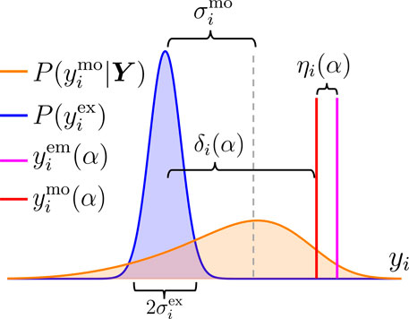
FIGURE 4. Visual representation of the statistical model with the three sources of uncertainty for an observable yi. For a particular value of α, the model calculation,
The experimental error, ϵi, is assumed to come from a normal distribution with mean zero and standard deviation
The modeling error, or model discrepancy term, δi(α), represents the intrinsic failures of the physical model when reproducing reality, for a given value of α. It is an aggregate of the many simplifications made during the construction of the model, as well as any physical effects, known or unknown, which are unaccounted for by the physical model. In the limit where the experimental errors become negligible, it is the term that explains the deviation between theory and observation. Due to these model limitations, we expect that even the best regions in the parameter space—values of α that make the discrepancies as small as possible—cannot make them all vanish simultaneously (δi(α) = 0) for every observable i.
It is typically unrealistic to expect a very precise estimate of the statistical properties of the set of δi(α) as α varies. Indeed, first, because the usual dataset in low-energy physics studies consist only of a few spherical magic or semi-magic nuclei, limiting the statistical analyses that can be made. Second, since the origin of δi(α) has roots in phenomena not completely understood, it becomes very hard to give accurate estimates when the experimental observations are not available. This motivates us to propose a parsimonious model, in accordance with the statistical principle that parsimony promotes robustness, an idea that traces back several decades (e.g. [75]). We assume that, up to scaling at the level of observables, the modeling error variances are shared within each of the two observable categories (binding energies and charge radii), and do not depend on the parameters α within their physical meaningful range that reproduces the nuclear properties. This is represented by the scale
Finally, for a given fixed value of the parameters α, the emulator error, ηi(α), represents the difference between the model’s original high fidelity calculation, and the approximate version computed by the emulator. In Figure 4 it is represented as the difference between the red and magenta vertical lines. This is the easiest error to obtain exactly, given a fixed α, since it is entirely computable, given access to the high fidelity and the emulator implementations. The challenge lies in estimating ηi(α) for new values of α without the use of the high fidelity solver. In the RBM literature, there exist approaches to estimate the emulator’s error in terms of the properties of the underlying differential equation [37], [76] and [77], but to our knowledge they have not been yet extended to the type of coupled nonlinear equations that describe our physical model Eq. 2 and Eq. 6. Our proposal below is to model all emulator errors, including the unobserved ones, using the same statistical model, where the emulator error intensity does not depend on α, thereby circumventing the issue of developing an analytical approach to extrapolating these errors in a non-linear setting, and keeping with the principle of parsimony.
Having identified and described these three sources of errors, we proceed to propose and implement methods to estimate their combined effect in order to calibrate our physical model properly through the RBM emulator.
In the case of binding energies and charge radii, the experimental determinations are precise enough that the typical error scale
We assume that the model discrepancies δi(α) scale proportionally to the value of each individual experimental datapoint. This is because each datapoint represents a different physical reality, and while, say, two binding energies for two similar nuclei may be subject to the same intensity of modeling error, this may not be a good assumption for two nuclei which are more distant in the nuclear landscape. Specifically, we assume that each scaled model discrepancies
And similarly for
where
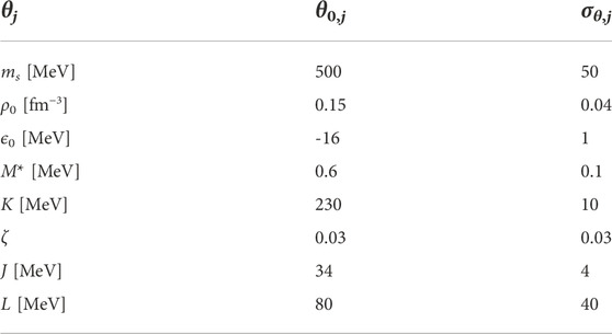
TABLE 2. Prior central values and standard deviations for the eight model parameters used in the calibration.
And
We express these two values as percentages since they are dimensionless. We treat the charge radius of 16O as an outlier and exclude it from this estimation, assigning it its own estimated error scale of
We follow a similar parsimonious approach and model the emulator error ηi(α) as coming from a normal distribution with mean zero and scale (standard deviation)
We estimate the scale
Under the assumptions we have made about the three sources of uncertainties, including the independence of all error terms which implies that the variance of their sum is the sum of their variances, we can finally specify the likelihood function for our statistical model. To simplify the prior specification and the exploration of the parameter space, we construct our statistical modeling using the bulk matter parametrization θ, which is equivalent to the Lagrangian couplings one with α (see Secion 2). Denoting N = NBE + NR = 18 and denoting by Y the N-dimensional vector formed of the experimental datapoints
Where
Our modeling assumptions about the error structure, plus the standardization in Y, imply indeed that χ2 is chi-squared distributed with N degrees of freedom. Note that
4.2 Prior
For the prior distribution we adopt an uncorrelated multivariate normal in θ as follows:
where:
The central values θ0,j and standard deviations σθ,j are specified for the eight components of θ in Table 2. They were chosen to roughly cover the expected parameter region with wide ranges based on the previous calibration [60].
4.3 Posterior
With our likelihood and priors fully set up, the posterior densities p.(θ|Y) for the parameters θ are given classically by Bayes’ rule [72] as being proportional to the product of the likelihood in Eq. 26 and the prior in Eq. 28, where the likelihood is evaluated at the experimentally observed datapoints labeled above as Y. From here, we are interested in using the Bayesian analysis to compare the calculations of the fully calibrated model with the experimental values of the observables, to verify that our uncertainty quantification is accurate. If our uncertainty bands on these predicted values are too narrow (too optimistic), too high a proportion of our 18 observations will fall outside of the bands. If our uncertainty bands are too wide (too conservative), many or all of our 18 observations will be inside their corresponding uncertainty bands. Being slightly too conservative is easily construed as a virtue to hedge against the risk of being too optimistic. The latter should be construed as an ill-reported uncertainty quantification. The method we propose here, to gauge the accuracy our uncertainty quantification, with results described in Section 5, is a manual/visual implementation of the now classical notion of Empirical Coverage Probability (ECP, see [73] for a nuclear physics implementation), appropriate for our very small dataset with 18 points. To compute the posterior density of every predicted value corresponding to our experimental observations, we view the likelihood model as a predictive model, featuring the fact that it includes statistical noise coming from the δ′s and η′s (see Figure 4 and Eq. 21), not just the posterior uncertainty in the parameters, and we simply use Bayesian posterior prediction, namely
where p (θ|Y) is the posterior density of all model parameters. In this fashion, the posterior uncertainty on the parameters, and the statistical uncertainty from the likelihood model, are both taken into account in a principled way. Note that this predictive calculation can be performed for all 20 observables of interest, though ECP-type comparisons with the experimental datapoints happen only for the 18 points we have, excluding charge radii for 100Sn and 68Ni. The next subsection explains how all Bayesian analyses are implemented numerically.
4.4 Metropolis-Hastings and surmise
The difficulty with any Bayesian method is to know how to understand the statistical properties of the posteriors. The simplest way to answer this question is to sample repeatedly (and efficiently) from those probability distributions. To sample from the posterior densities of the model parameters θ, we use the standard Metropolis-Hastings algorithm implemented in the surmise Python package [80]. For the results presented here, eight independent chains of 725,000 samples were ran using the direct Bayes calibrator within surmise. For the step size used, the ratio of acceptance for proposed new steps was about 30% across all chains. The first 100,000 samples of each chain were taken as a burn-in, reducing the effective sample size of the calibration to 5,000,000 evaluations. The eight chains were run in parallel and thus the 5,800,000 total evaluations took about a day on a personal computer with commodity hardware. For comparison, it would have taken nearly 6 years of continuous computation to produce the same results using the original code for the high-fidelity model.
To evaluate posterior predictive distributions to compare with the experimental data, we rely on the fact that surmise, like any flexible Monte-Carlo Bayesian implementation, gives us access to all Metropolis-Hastings samples. For each multivariate sample of the parameters in θ, we draw independent samples from the normal distributions in the likelihood model Eq. 21, and evaluate the corresponding value of
5 Results and discussion
Having defined the covariant density functional model in Secion 2, the reduced basis emulator in Secion 3, and the statistical framework and the computational sampling tools in Secion 4 we are in position to use the experimental data to calibrate the model under a Bayesian approach. At the time of the original calibration of the FSUGold2 functional [60], this would have represented an exceptional computational challenge, mainly because of the absence of the computational speed up of three orders of magnitude provided by the RBM. Instead, in the original calibration, one was limited to finding the minimum of the objective (or χ2) function and the matrix of second derivatives. In this manner, it was possible to compute uncertainties and correlations between observables, but only in the Gaussian approximation. We compare and contrast our results and procedure, highlighting that with the exception of the information on the four giant monopole resonances and the maximum neutron star mass, both calibrations share the same dataset of binding energies and charge radii.
We begin by displaying in graphical form the results of our Bayesian implementation in surmise as a corner plot in Figure 5. The corner plot summarizes the posterior distribution of bulk parameters alongside the two-dimensional correlations. For comparison, the Gaussian distribution of parameters extracted from the original FSUGold2 calibration is displayed by the vertically scaled blue line. As expected, the width of the one-dimensional distributions has increased—in some cases significantly—relative to the Gaussian approximation that is limited to explore the parameter landscape in the vicinity of the χ2 minimum. The inclusion of bigger estimated model errors δi in Eq. 21 likely also share responsibility for the increased overall uncertainty. Besides the increase in the width of the distribution, we see a relatively significant shift in the average value of the incompressibility coefficient K. We attribute this fact to the lack of information on the GMR, which is the observable that is mostly sensitive to K.
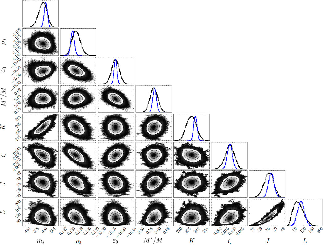
FIGURE 5. Corner plot [81] from the posterior distribution of the eight bulk matter parameters θ obtained from the Metropolis-Hasting sampling with surmise. A total of five million samples were used, distributed along eight independent chains. The saturation density ρ0 is expressed in fm−3, the mass of the σ meson ms, the binding energy at saturation ɛ0, the incompressibility coefficient K, the symmetry energy J and its slope L at saturation are all expressed in MeV. For comparison, the original calibration done in [60] is shown as the blue curves along the diagonal, scaled vertically to fit in the same plot as our posterior results in black.
Beyond the corner plot that displays the distribution of bulk parameters and the correlations among them, we illustrate in Figure 6 and Table 3 the performance of the model as compared with the experimental data informing the calibration. Note that in Figure 6 as well as in Table 3 we have defined the binding energy as a positive quantity.
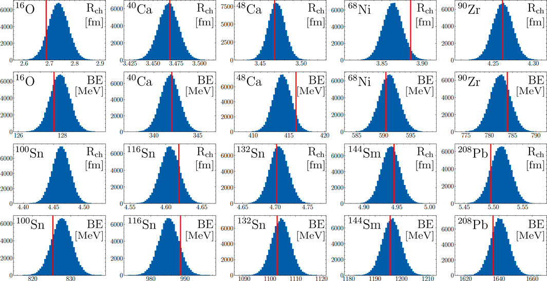
FIGURE 6. Posterior distributions for the binding energies (in MeV) and charge radii (in fm) of the ten nuclei involved in our study. A total of 100,000 samples from the 5,000,000 visited parameter values were used to make these distributions. The vertical red line in each plot represents the associated experimental values, all contained within the 95% credible interval of the model, including the charge radii of 68Ni which was not included in the calibration of the model. On the other hand, 100Sn does not have a measured charge radius, making its associated posterior distribution a true prediction from our calibration. The numerical values for the mean and credible intervals on all these quantities are displayed in Table 3.
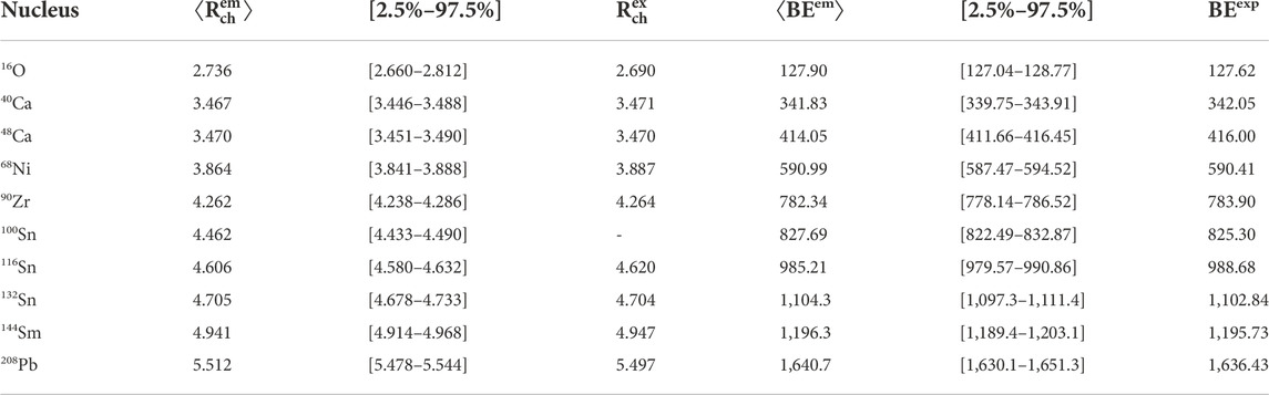
TABLE 3. Mean values and 95% credible intervals of the Bayesian posteriors on charge radii (in fm) and binding energy (in MeV), showed in Figure 6. Also displayed are the 19 available experimental values [60, 63]. The credible intervals are calculated as equal-tailed intervals—such that the probabilities of falling above or below the interval are both equal to 2.5%.
The blue histograms display the posterior predictive distributions Eq. 30 of each of the 20 observables. Included in our results is the prediction for the yet to be measured charge radius of 100Sn, as well as the charge radius of 68Ni not used in the calibration. The vertical red lines indicate the values of the experimental datapoints specified in [60] and [63]. These plots show excellent coverage of all datapoints within our reported uncertainty. With 19 datapoints, one would expect about one of them to fall outside of 95% credible intervals. The credible intervals are printed in Table 3, showing that none of our datapoints fall outside those intervals around the posterior means. This implies that our uncertainty quantification leans towards the conservative side, although the binding energy for 48Ca and the charge radii of 68Ni are very close to falling outside the 95% band. Our method has produced uncertainties which are very likely not to be overly wasteful by significantly over-reporting uncertainty, and which are very likely not to under-report uncertainty. This is exactly where a Bayesian predictive posterior coverage analysis wants to be in a study with such a small number of datapoints.
Being the lightest of all the nuclei included in the calibration, 16O may be regarded as a questionable “mean-field” nucleus. As such, comparing its experimental charge radius with our posterior results is particularly interesting, since the model standard deviation we used was more than 5 times larger than for the other observables. Yet, our reported uncertainty sees the experimental measurement fairly well reproduced. This is an indication that it was important to use the higher model variance, or our prediction could have reported too low of an uncertainty. Using a smaller variance for the model error δi could have also pushed the parameters too strongly towards the 16O charge radius outlier, deteriorating the overall performance of the calibration on the other nuclei. The final coverage of all data points illustrates our method’s ability to handle heteroskedasticity (uneven variances) well. Finally, in Figure 6, because our comparison with predictive distributions performs very well and is only mildly conservative, we can be confident that our prediction for the charge radii of 100Sn is robust. How narrow these histograms are is a testament to the quality of the original modeling, its emulation, and our uncertainty quantification.
Coming back to the corner plot in Figure 5, we note that the strongest correlation between observables involves the value of the symmetry energy (J) and its slope (L) at saturation density. The symmetry energy quantifies the energy cost in transforming symmetric nuclear matter—with equal number of neutrons and protons—to pure neutron matter. In the vicinity of nuclear matter saturation density, one can expand the symmetry energy in terms of a few bulk parameters [82]:
where x = (ρ − ρ0)/3ρ0 is a dimensionless parameter that quantifies the deviations of the density from its value at saturation. Given that the calibration is informed by the binding energy of neutron-rich nuclei, such as 132Sn and 208Pb, the symmetry energy
Hence, accurately calibrated EDFs display a strong correlation between J and L by the mere fact that the calibration included information on the binding energy of neutron-rich nuclei. In the original calibration of FSUGold2 [60], one obtained a correlation coefficient between J and L of 0.97, while in this work we obtained a correlation coefficient of 0.92. The slight non-linearity observed in Figure 5 on the correlation between J and L is due to Ksym, which was neglected in the simple argument made in Eq. 32.
Although not directly an observable, L has been determined to be strongly correlated to the thickness of the neutron skin of heavy nuclei [83–85]; the neutron skin thickness is defined as the difference in the mean square radii between the neutron and proton vector densities (see Eq. 8). In Figure 7 we show the correlation plot between L and the neutron skin of 48Ca and 208Pb calculated directly from 100,000 random samples from our posterior distributions. It is important to note that we have not included the model error δi through Eq. 30 in these histograms9, and as such we do not expect the uncertainties to be accurate, as we discuss later in Sec. VI.
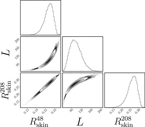
FIGURE 7. Correlation corner plot [81] between the posterior distributions for the neutron skin of 48Ca and 208Pb (both in fm), and the slope of the symmetry energy L (in MeV). A total of 100,000 samples from the 5,000,000 visited parameter values were used to make these distributions. Both neutron skins
The correlation between L and the thickness of the neutron skin of heavy nuclei has a strong physical underpinning. For example, in the case of 208Pb, surface tension favors the formation of a spherical liquid drop containing all 208 nucleons. However, the symmetry energy increases monotonically in the density region of relevance to atomic nuclei. Hence, to minimize the symmetry energy, is energetically favorable to move some of the excess neutrons to the surface. It is then the difference in the symmetry energy at the core relative to its value at the surface that determines the thickness of the neutron skin; such a difference is encoded in the slope of the symmetry energy L. If such a difference is large enough to overcome surface tension, then some of the excess neutrons will be pushed to the surface, resulting in a thick neutron skin [86]. That the correlation between the neutron skin thickness of 208Pb and L is strong has been validated using a large set of EDFs [85]. Note that L is closely related to the pressure of pure neutron matter at saturation density—a quantity that has been extensively studied using chiral effective field theory [13–19], and which is of great relevance to our understanding of the structure of neutron stars [87].
It is important to note that no information on neutron skins—or any other observable that is strongly correlated to L—was included in our calibration procedure, making it difficult to estimate the model error associated with such quantities. This also indicates that in the absence of any guidance, the class of covariant EDFs used in this work tend to produce stiff symmetry energies, in contrast to Skyrme-type EDFs and chiral effective field theories that tend to favor relatively soft symmetry energies [13–19, 88]. Particularly interesting to note is that whereas
Given the recently reported results from the PREX-II [48] and CREX [49] experimental campaigns, our model’s average predicted neutron skin for both 208Pb (0.27 fm) and 208Ca (0.23 fm) might indicate that the physics encapsulated in the Lagrangian density depicted in Eq. 1 is insufficient to describe both skins simultaneously. Granted, with only two isovector parameters the model may be too rigid to break the strong observed model correlation between
To make a clear assessment, we will need to both include a statistical treatment of the expected model error in these quantities, as well as mitigate possible model dependencies by directly comparing with experimental observations such as the parity violating asymmetry. We are planing to do so as an immediate direction by calibrating covariant EDFs with an extended and more elaborated isovector sector that might help bridge both neutron skin results without compromising the success of the model in reproducing other nuclear observables, such as the ones displayed in Figure 6. As we discuss in the next and final section, well quantified uncertainties enabled by powerful emulators such as the RBM will be indispensable to achieve those goals and make full use of the anticipated new laboratory experiments and astronomical observations that will be coming in the next years.
6 Conclusion and outlook
In the last few decades nuclear theory has gone through several transformational changes brought on by embracing philosophies and techniques from the fields of statistics and computational science. It is now expected that theoretical predictions should always be accompanied by uncertainties [93]. This is particularly true in theoretical nuclear physics where predictions from QCD inspired models require the calibration of several model parameters. This newly-adopted philosophy has also prompted the exploration of uncertainty quantification across the many sub-fields of nuclear theory [34, 94–97]. Furthermore, several recent advancements and discoveries have become feasible only through the successful integration of machine learning and other novel computational approaches to the large body of theoretical models developed over many decades [31, 74, 98–100]. This dedication is also exemplified by the theory community’s proactive efforts to organize topical conferences, summer schools, and workshops in service of disseminating the technical know-how to every level of the community.
Aligned with these developments and efforts, our present work aimed at showcasing a pipeline for integrating a statistical framework through one such innovative computational technique. We have calibrated a covariant energy density functional within a Bayesian approach using available experimental values of binding energies and charge radii. The calibration of the model, as well as the quantification of the uncertainties of its predictions, required millions of evaluations for different values of its parameters. Such titanic computational burden was made possible—straightforward even—thanks to the emulation of the model through the reduced basis method, which decreased the necessary calculation time from months or years to a single day on a personal computer.
Our calibration’s main results, which consists of posterior distributions for all the model’s parameters, were presented in Figure 5. From these posteriors, and following the statistical framework we developed in Sec. IV, the model output can be estimated with well quantified uncertainties that can take into account experimental, model, and emulator errors. We showed such calculations with their respective estimated uncertainties in Figure 6 and Table 3 for the binding energies and charge radii of the 10 nuclei involved in the study. The fact that the experimental values used in the calibration, depicted as red vertical lines in Figure 6, fall within the 95% our calculated credible intervals gives us confidence that our uncertainty procedure was not biased towards being too optimistic for this dataset. This is especially true for the case of the charge radii of 16O, which was treated as an outlier based on prior expert knowledge on the expectation of the limits of the mean field approach for smaller systems. Once the experimental value for the charge radii of 100Sn becomes available, it will be interesting to contrast our model prediction’s and gauge the success of the uncertainty level estimated.
However, the picture changes when we focus on the calculations for the neutron skin thickness of 48Ca and 208Pb showed in Figure 7. The recent experimental campaigns PREX [101], PREX-II [102], and CREX [49] on parity violating electron scattering have published results which suggest that the neutron skins of 48Ca and 208Pb stand in opposite corners. While 208Pb is estimated to have a relatively thick neutron skin of around 0.28 fm [102], 48Ca [49] is estimated to have a significantly smaller skin of around 0.12 fm. Albeit we have not included a model error term in the calculations shown in Figure 7, it seems that our current model is unable to satisfy both values simultaneously.
Moving forward, we envision two complementary research directions that could help mitigate the problems identified above. First, one could build a more robust statistical framework that, by including strong isovector indicators, such as information on the electric dipole response of neutron rich nuclei, will impose stringent constraints on the isovector sector. Second, and as already mentioned, we could increase the flexibility of the isovector sector by adding additional interactions that modify the density dependence of the symmetry energy. The use of dimensionality reduction techniques such as the RBM to significantly speed up the calculation time—especially if information on nuclear excitations is incorporated into the calibration of the EDF—will become a fundamental pillar of the fitting protocol.
We believe that the RBM we showcased here has the potential to further impact many of the nuclear theory areas that have already made use of similar emulators, as well as expanding the frontiers of the physical models that can be successfully emulated. Indeed, the RBM’s unique combination of few high-fidelity evaluations needed to build an effective emulator, the simplicity and flexibility of the Galerkin projection, and the ability to precompute many observables and equations in the offline stage could allow the community to deploy trained emulators for use on different computer architectures and on cloud infrastructure [103]. This could effectively lower the barrier created by the need of running expensive computer models locally. This could give access of cutting edge theoretical models and simulations to an increased number of research groups, opening new opportunities to expand the network of collaborative research.
In short, the computational framework detailed in this work attempts to provide an end-to-end solution for model calibration and exploration with a focus on statistical rigor without sacrificing computational efficiency. By leveraging this efficiency to nimbly incorporate new experimental data, one can imagine the continuous calibration of models that can be updated in a matter of hours without requiring large-scale computing facilities. Finally, the heavy focus on integrating these disparate parts into a user-friendly form to generate physics-informed emulators is ultimately in service of our wider goal to increase data availability and software accessibility, and is a necessity in the paradigmatic shift towards probability distributions—rooted in Bayesian principles—defining physical models rather than a single set of optimal parameters.
Data availability statement
The datasets presented in this study can be found in online repositories. The names of the repository/repositories and accession number(s) can be found below: https://figshare.com/projects/RBM_Calibration_Pipeline/149840.
Author contributions
PG, KG, and EB created the RBM framework. PG and KG implemented the computational pipeline. PG and FV created the Statistical Framework. KG created the computational sampling framework. JP provided the RMF physical description and insight and created the Relativistic Mean Field original code. All authors contributed to the writing and editing of the manuscript.
Funding
This work was supported by the National Science Foundation CSSI program under award number 2004601 (BAND collaboration) and the U.S. Department of Energy under Award Numbers DOE-DE-NA0004074 (NNSA, the Stewardship Science Academic Alliances program), DE-SC0013365 (Office of Science), and DE-SC0018083 (Office of Science, NUCLEI SciDAC-4 collaboration). This material is based upon work supported by the U.S. Department of Energy Office of Science, Office of Nuclear Physics under Award Number DE-FG02-92ER40750.
Acknowledgments
We are grateful to Moses Chan for guiding us on the use of the surmise python package, as well as for useful discussions and recommendations on good practices for the Monte Carlo sampling. We are grateful to Craig Gross for useful discussions about the reduced basis method, including the visualization of the speed up gained in terms of the high fidelity solver size
Conflict of interest
The authors declare that the research was conducted in the absence of any commercial or financial relationships that could be construed as a potential conflict of interest.
Publisher’s note
All claims expressed in this article are solely those of the authors and do not necessarily represent those of their affiliated organizations, or those of the publisher, the editors and the reviewers. Any product that may be evaluated in this article, or claim that may be made by its manufacturer, is not guaranteed or endorsed by the publisher.
Footnotes
1The charge radius of 68Ni was recently measured [63] and we do not include in the calibration to better compare with the previous results [60]. The charge radius of 100Sn has not been measured yet. Therefore, our calibration dataset consists of 18 points, 10 binding energies and 8 charge radii.
2Both the grid size and the step size could be adaptive instead of constant across the spatial domain. We shall assume a constant Δr for the rest of the discussion for the sake of simplicity.
3With an error of around 1.4%, the charge radius of 16O can be treated as an outlier in which the mean field approximation might break down.
4If the dependence on the parameters α of the operators involved in the system’s equations, or in the observable’s calculations is not affine, techniques such as the Empirical Interpolation Method [37, 69, 70] can be implemented to avoid computations of size
5For some steps the emulator’s performance -in terms of Δ Rch and Δ BE-gets worse when adding the four new basis, which at first might seem counter-intuitive. It is important to note, however, that with each new basis we add we are changing the entire system of equations both by adding four new projections and by adding new elements to the previous ones. Nothing prevents the solution a to the new system to under perform in comparison to the previous one in the particular metric we are using.
6A fourth source of error could be, in principle, the computational error in the high fidelity solver for the physical model. We expect this error to be negligible in comparison to the other three at the level of resolution Δr our high fidelity solvers have.
7For example, the binding energy of 208Pb is known to a precision better than 10–4% [78], while its charge radius to a precision of 0.02% [79]. In contrast, the estimated model error we calculate in the following discussion for the same quantities is 0.25% and 0.26%, respectively.
8The experimental values of the charge radii for 68Ni was not known at the time of the calibration in [60], while the charge radii of 100Sn is still not known. In these cases, we used the values reported for FSUGold2 as proxies to preserve these two nuclei in the analysis when creating predictive posterior distributions with the calibrated model.
9Such procedure would require to first give an accurate estimation of the model error on neutron radii -a non trivial task given the lack of experimental data on neutron radii-, and second to take into account the model correlation between Rp and Rn.
References
2. Abbott BP. LIGO scientific collaboration, virgo collaboration. Phys Rev Lett (2017) 119:161101. doi:10.1103/physrevlett.121.129902
3. Drout MR, Piro AL, Shappee BJ, Kilpatrick CD, Simon JD, Contreras C, et al. Light curves of the neutron star merger GW170817/SSS17a: Implications for r-process nucleosynthesis. Science (2017) 358:1570. doi:10.1126/science.aaq0049
4. Cowperthwaite PS, Berger E, Villar VA, Metzger BD, Nicholl M, Chornock R, et al. The electromagnetic counterpart of the binary neutron star merger LIGO/virgo GW170817. II. UV, optical, and near-infrared light curves and comparison to kilonova models. Astrophys J (2017) 848:L17. doi:10.3847/2041-8213/aa8fc7
5. Chornock R, Berger E, Kasen D, Cowperthwaite PS, Nicholl M, Villar VA, et al. The electromagnetic counterpart of the binary neutron star merger LIGO/virgo GW170817. IV. Detection of near-infrared signatures of r-process nucleosynthesis with gemini-south. Astrophys J (2017) 848:L19. doi:10.3847/2041-8213/aa905c
6. Nicholl M, Berger E, Kasen D, Metzger BD, Elias J, Briceño C, et al. The electromagnetic counterpart of the binary neutron star merger LIGO/virgo GW170817. III. Optical and UV spectra of a blue kilonova from fast polar ejecta. Astrophys J (2017) 848:L18. doi:10.3847/2041-8213/aa9029
7. Fattoyev FJ, Piekarewicz J, Horowitz CJ. Neutron skins and neutron stars in the multimessenger era. Phys Rev Lett (2018) 120:172702. doi:10.1103/physrevlett.120.172702
8. Annala E, Gorda T, Kurkela A, Vuorinen A. Gravitational-wave constraints on the neutron-star-matter equation of state. Phys Rev Lett (2018) 120:172703. doi:10.1103/physrevlett.120.172703
9. Abbott BP. LIGO scientific collaboration, virgo collaboration). Phys Rev Lett (2018) 121:161101. doi:10.1103/physrevlett.121.129902
10. Weinberg S. Nuclear forces from chiral Lagrangians. Phys Lett B (1990) 251:288–92. doi:10.1016/0370-2693(90)90938-3
11. van Kolck U. Few-nucleon forces from chiral Lagrangians. Phys Rev C (1994) 49:2932–41. doi:10.1103/physrevc.49.2932
12. Ordóñez C, Ray L, van Kolck U. Two-nucleon potential from chiral Lagrangians. Phys Rev C (1996) 53:2086–105. doi:10.1103/physrevc.53.2086
13. Hebeler K, Schwenk A. Chiral three-nucleon forces and neutron matter. Phys Rev C (2010) 82:014314. doi:10.1103/physrevc.82.014314
14. Tews I, Kruger T, Hebeler K, Schwenk A. Neutron matter at next-to-next-to-next-to-leading order in chiral effective field theory. Phys Rev Lett (2013) 110:032504. doi:10.1103/physrevlett.110.032504
15. Kruger T, Tews I, Hebeler K, Schwenk A. Neutron matter from chiral effective field theory interactions. Phys Rev (2013) C88:025802. doi:10.1103/PhysRevC.88.025802
16. Lonardoni D, Tews I, Gandolfi S, Carlson J. Nuclear and neutron-star matter from local chiral interactions. Phys Rev Res (2020) 2:022033. doi:10.1103/physrevresearch.2.022033
17. Drischler C, Holt JW, Wellenhofer C. Chiral effective field theory and the high-density nuclear equation of state. Annu Rev Nucl Part Sci (2021) 71:403–32. doi:10.1146/annurev-nucl-102419-041903
18. Sammarruca F, Millerson R. Overview of symmetric nuclear matter properties from chiral interactions up to fourth order of the chiral expansion. Phys Rev C (2021) 104:034308. doi:10.1103/physrevc.104.064312
19. Millerson F, Millerson R. The equation of state of neutron-rich matter at fourth order of chiral effective field theory and the radius of a medium-mass neutron star. Universe (2022) 8:133. doi:10.3390/universe8020133
20. Kohn W. Nobel Lecture: Electronic structure of matter-wave functions and density functionals. Rev Mod Phys (1999) 71:1253–66. doi:10.1103/revmodphys.71.1253
21. Kohn P, Kohn W. Inhomogeneous electron gas. Phys Rev (1964) 136:B864–B871. doi:10.1103/physrev.136.b864
22. Sham W, Sham LJ. Self-consistent equations including exchange and correlation effects. Phys Rev (1965) 140:A1133–A1138. doi:10.1103/physrev.140.a1133
23. Phillips DR, Furnstahl RJ, Heinz U, Maiti T, Nazarewicz W, Nunes FM, et al. Get on the BAND wagon: A bayesian framework for quantifying model uncertainties in nuclear dynamics. J Phys G: Nucl Part Phys (2021) 48:072001. doi:10.1088/1361-6471/abf1df
24. Frame D, He R, Ipsen I, Lee D, Lee D, Rrapaj E. Eigenvector continuation with subspace learning. Phys Rev Lett (2018) 121:032501. doi:10.1103/physrevlett.121.032501
25. König S, Ekström A, Hebeler K, Lee D, Schwenk A. Eigenvector continuation as an efficient and accurate emulator for uncertainty quantification. Phys Lett B (2020) 810:135814. doi:10.1016/j.physletb.2020.135814
26. Furnstahl R, Garcia A, Millican P, Zhang X. Efficient emulators for scattering using eigenvector continuation. Phys Lett B (2020) 809:135719. doi:10.1016/j.physletb.2020.135719
27. Melendez J, Drischler C, Garcia A, Furnstahl R, Zhang X. Fast & accurate emulation of two-body scattering observables without wave functions. Phys Lett B (2021) 821:136608. doi:10.1016/j.physletb.2021.136608
28. Drischler C, Quinonez M, Giuliani P, Lovell A, Nunes F. Toward emulating nuclear reactions using eigenvector continuation. Phys Lett B (2021) 823:136777. doi:10.1016/j.physletb.2021.136777
29. Bonilla E, Giuliani P, Godbey K, Lee D, (2022), Training and projecting: A reduced basis method emulator for many-body physics. Phys Rev C (2022) 106:054322. doi:10.1103/PhysRevC.106.054322
30. Sarkar A, Lee D. Self-learning emulators and eigenvector continuation. Phys Rev Res (2022) 4:023214. doi:10.1103/physrevresearch.4.023214
31. Boehnlein A, Diefenthaler M, Sato N, Schram M, Ziegler V, Fanelli C, et al. Colloquium: Machine learning in nuclear physics. Rev Mod Phys (2022) 94:031003. doi:10.1103/revmodphys.94.031003
32. Tews I, Davoudi Z, Ekström A, Holt JD, Becker K, Briceño R, et al. Nuclear forces for precision nuclear physics: A collection of perspectives. Few-body Syst (2022) 63:1. doi:10.1007/s00601-022-01749-x
33. Higdon D, McDonnell JD, Schunck N, Sarich J, Wild SM. A Bayesian approach for parameter estimation and prediction using a computationally intensive model. J Phys G Nucl Part Phys (2015) 42:034009. doi:10.1088/0954-3899/42/3/034009
34. McDonnell JD, Schunck N, Higdon D, Sarich J, Wild SM, Nazarewicz W. Uncertainty quantification for nuclear density functional theory and information content of new measurements. Phys Rev Lett (2015) 114:122501. doi:10.1103/physrevlett.114.122501
35. Anderson AL, O'Donnell GL, Piekarewicz J. Applications of reduced-basis methods to the nuclear single-particle spectrum. Phys Rev C (2022) 106:L031302. doi:10.1103/physrevc.106.l031302
36. Quarteroni A, Manzoni A, Negri F. Reduced basis methods for partial differential equations: An introduction, 92. Springer (2015). doi:10.1007/978-3-319-15431-2
37. Hesthaven JS, Rozza G, Stamm B. Certified reduced basis methods for parametrized partial differential equations, 590. Springer (2016). doi:10.1007/978-3-319-22470-1
38. Melendez JA, Drischler C, Furnstahl RJ, Garcia AJ, Zhang X. Model reduction methods for nuclear emulators. J Phys G: Nucl Part Phys (2022) 49:102001. doi:10.1088/1361-6471/ac83dd
39. Quarteroni A, Rozza G. Reduced order methods for modeling and computational reduction, 9. Springer (2014). doi:10.1007/978-3-319-02090-7
40. Brunton SL, Kutz JN. Data-driven science and engineering: Machine learning, dynamical systems, and control. Cambridge University Press (2019). doi:10.1017/9781108380690
41. Benner P, Gugercin S, Willcox K. A survey of projection-based model reduction methods for parametric dynamical systems. SIAM Rev (2015) 57:483–531. doi:10.1137/130932715
42. Sartori A, Cammi A, Luzzi L, Rozza G. A reduced basis approach for modeling the movement of nuclear reactor control rods. J Nucl Eng Radiat (2016) 2:1062. doi:10.1115/1.4031945
43. Quarteroni A, Rozza G, Manzoni A. Certified reduced basis approximation for parametrized partial differential equations and applications. J Math Ind (2011) 1:1. doi:10.1186/2190-5983-1-3
44. Field SE, Galley CR, Herrmann F, Hesthaven JS, Ochsner E, Tiglio M. Reduced basis catalogs for gravitational wave templates. Phys Rev Lett (2011) 106:221102. doi:10.1103/physrevlett.106.221102
45. Nguyen NC, Rozza G, Huynh DBP, Patera AT. Reduced basis approximation and a posteriori error estimation for parametrized parabolic PDEs: Application to real-time bayesian parameter estimation. In: Large-scale inverse problems and quantification of uncertainty. John Wiley & Sons (2010). p. 151–77. Chap. 8. doi:10.1002/9780470685853.ch8
46. Jiang J, Chen Y, Narayan A. A goal-oriented reduced basis methods-accelerated generalized polynomial chaos algorithm. Siam/asa J Uncertainty Quantification (2016) 4:1398–420. doi:10.1137/16m1055736
47. Abrahamyan S, Ahmed Z, Albataineh H, Aniol K, Armstrong DS, Armstrong W. Measurement of the neutron radius of 208Pb through parity violation in electron scattering. Phys Rev Lett (2012) 108:112502. doi:10.1103/PhysRevLett.108.112502
48. Adhikari D. Accurate determination of the neutron skin Th. Phys Rev Lett (2021) 126:172502. doi:10.1103/PhysRevLett.126.172502
49. Adhikari D. Precision determination of the neutral weak form factor of 48 Ca. Phys Rev Lett (2022) 129:042501. doi:10.1103/PhysRevLett.129.042501
50. Reed BT, Fattoyev FJ, Horowitz CJ, Piekarewicz J. Implications of PREX-2 on the equation of state of neutron-rich matter. Phys Rev Lett (2021) 126:172503. doi:10.1103/physrevlett.126.172503
51. Reinhard P-G, Roca-Maza X, Nazarewicz W, Combined theoretical analysis of the parity-violating asymmetry for 48Ca and 208Pb. (2022), arXiv:2206.03134 [nucl-th] .
52. Ireland D, Nazarewicz W. Enhancing the interaction between nuclear experiment and theory through information and statistics. J Phys G Nucl Part Phys (2015) 42. doi:10.1088/0954-3899/42/3/030301
53. Bedaque P, Boehnlein A, Cromaz M, Diefenthaler M, Elouadrhiri L, Horn T, et al. Eur Phys J A (2021) 57:1. doi:10.1140/epja/s10050-020-00290-x
54. Walecka JD. A theory of highly condensed matter. Ann Phys (1974) 83:491–529. doi:10.1016/0003-4916(74)90208-5
55. Serot BD, Walecka JD. Relativistic nuclear many-body theory. Adv Nucl Phys (1986) 16:1. doi:10.1007/978-1-4615-3466-2_5
56. Bodmer J, Bodmer AR. Relativistic calculation of nuclear matter and the nuclear surface. Nucl Phys A (1977) 292:413–28. doi:10.1016/0375-9474(77)90626-1
57. Mueller H, Serot BD. Relativistic mean-field theory and the high-density nuclear equation of state. Nucl Phys A (1996) 606:508. doi:10.1016/0375-9474(96)00187-X
58. Piekarewicz CJ, Piekarewicz J. Neutron star structure and the neutron radius ofP208b. Phys Rev Lett (2001) 86:5647–50. doi:10.1103/physrevlett.86.5647
59. Todd BG, Piekarewicz J. Relativistic mean-field study of neutron-rich nuclei. Phys Rev C (2003) 67:044317. doi:10.1103/physrevc.67.044317
60. Chen W-C, Piekarewicz J. Building relativistic mean field models for finite nuclei and neutron stars. Phys Rev C (2014) 90:044305. doi:10.1103/physrevc.90.044305
61. Piekarewicz J, Piekarewicz J. Covariant density functional theory in nuclear physics and astrophysics. Annu Rev Nucl Part Sci (2020) 70:21–41. doi:10.1146/annurev-nucl-101918-023608
62. Tiesinga E, Mohr PJ, Newell DB, Taylor BN. CODATA recommended values of the fundamental physical constants: 2018. J Phys Chem Reference Data (2021) 50:033105. doi:10.1063/5.0064853
63. Kaufmann S, Simonis J, Bacca S, Billowes J, Bissell ML, Blaum K. Charge radius of the short-lived Ni 68 and correlation with the dipole plarizability. (2020). Phys Rev Lett (2012) 124:132502. doi:10.1103/PhysRevLett.127.182503
65. Blum A, Hopcroft J, Kannan R. Foundations of data science. Cambridge University Press (2020). doi:10.1017/9781108755528
67. Rawitscher G, dos Santos Filho V, Peixoto TC. Galerkin and collocation methods. In: An introductory guide to computational methods for the solution of physics problems. Springer (2018). p. 17–31. doi:10.1007/978-3-319-42703-4
69. Grepl MA, Maday Y, Nguyen NC, Patera AT. Efficient reduced-basis treatment of nonaffine and nonlinear partial differential equations. Esaim: M2an (2007) 41:575–605. doi:10.1051/m2an:2007031
70. Barrault M, Maday Y, Nguyen NC, Patera AT. An 'empirical interpolation' method: Application to efficient reduced-basis discretization of partial differential equations. Comptes Rendus Mathematique (2004) 339:667–72. doi:10.1016/j.crma.2004.08.006
71. Virtanen P, Gommers R, Oliphant TE, Haberland M, Reddy T, Cournapeau D, et al. SciPy 1.0: Fundamental algorithms for scientific computing in Python. Nat Methods (2020) 17:261–72. doi:10.1038/s41592-019-0686-2
72. Gelman A, Carlin JB, Stern HS, Rubin DB. Bayesian data analysis. Chapman and Hall/CRC (1995). doi:10.1201/b16018
73. Neufcourt L, Cao Y, Nazarewicz W, Viens F. Bayesian approach to model-based extrapolation of nuclear observables. Phys Rev C (2018) 98:034318. doi:10.1103/physrevc.98.034318
74. Neufcourt L, Cao Y, Nazarewicz W, Olsen E, Viens F. Neutron drip line in the Ca region from bayesian model averaging. Phys Rev Lett (2019) 122:062502. doi:10.1103/physrevlett.122.062502
76. Veroy K, Prud’Homme C, Rovas D, Patera A. A posteriori error bounds for reduced-basis approximation of parametrized noncoercive and nonlinear elliptic partial differential equations. Fluid Dyn Conf (2003) 3847. 16th AIAA Comput. doi:10.2514/6.2003-3847
77. Buffa A, Maday Y, Patera AT, Prud’homme C, Turinici G. A prioriconvergence of the Greedy algorithm for the parametrized reduced basis method. Esaim: M2an (2012) 46:595–603. doi:10.1051/m2an/2011056
78. Huang W, Wang M, Kondev FG, Audi G, Naimi S. The AME 2020 atomic mass evaluation (I). Evaluation of input data, and adjustment procedures*. Chin Phys. C (2021) 45:030002. doi:10.1088/1674-1137/abddb0
79. Marinova I, Marinova KP. Table of experimental nuclear ground state charge radii: An update. At Data Nucl Data Tables (2013) 99:69–95. doi:10.1016/j.adt.2011.12.006
80. Plumlee M, Sürer Ö, Wild SM. Tech. Rep. Version 0.1.0. NAISE (2021). Surmise users manual. Available at: https://surmise.readthedocs.io/en/latest/introduction.html
81. Foreman-Mackey D. corner.py: Scatterplot matrices in Python. Joss (2016) 1:24. doi:10.21105/joss.00024
82. Piekarewicz J, Centelles M. Incompressibility of neutron-rich matter. Phys Rev C (2009) 79:054311. doi:10.1103/physrevc.79.054311
83. Furnstahl RJ. Neutron radii in mean-field models. Nucl Phys A (2002) 706:85–110. doi:10.1016/s0375-9474(02)00867-9
84. Brown BA. Neutron radii in nuclei and the neutron equation of state. Phys Rev Lett (2000) 85:5296–9. doi:10.1103/PhysRevLett.85.5296
85. Roca-Maza X, Centelles M, Viñas X, Warda M. Neutron skin ofPb208, nuclear symmetry energy, and the parity radius experiment. Phys Rev Lett (2011) 106:252501. doi:10.1103/physrevlett.106.252501
86. Horowitz CJ, Piekarewicz J. The neutron radii of Lead and neutron stars. Phys Rev C (2001) 64:062802. doi:10.1103/physrevc.64.062802
87. Fattoyev J, Fattoyev FJ. Neutron-rich matter in heaven and on Earth. Phys Today (2019) 72:30–7. doi:10.1063/pt.3.4247
88. Reinhard P-G, Roca-Maza X, Nazarewicz W. Information content of the parity-violating asymmetry in Pb208. Phys Rev Lett (2021) 127:232501. doi:10.1103/physrevlett.127.232501
89. Piekarewicz J. Implications of PREX-2 on the electric dipole polarizability of neutron-rich nuclei. Phys Rev C (2021) 104:024329. doi:10.1103/physrevc.104.024329
90. Hu B, Jiang W, Miyagi T. Ab initio predictions link the neutron skin of 208Pb to nuclear forces. Nat Phys (2022) 18:1196–200. doi:10.1038/s41567-022-01715-8
91. Zhang Z, Chen L-W, (2022), Bayesian inference of the symmetry energy and the neutron skin in 48Ca and 208Pb from CREX and PREX-2, arXiv:2207.03328 [nucl-th].
92. Mondal C, Gulminelli F, (2022), Nucleonic metamodelling in light of multimessenger, PREX-II and CREX data, arXiv:2209.05177 [nucl-th].
93. Join A. A new mass model for nuclear astrophysics: Crossing 200 keV accuracy. Phys Rev A (2011) 83:040001.
94. Godbey K, Umar S, Simenel C. Theoretical uncertainty quantification for heavy-ion fusion. Phys Rev C. (2022) 106:L0511602. doi:10.1103/PhysRevC.106.L051602
95. King G, Lovell A, Neufcourt L, Nunes F. Direct comparison between bayesian and frequentist uncertainty quantification for nuclear reactions. Phys Rev Lett (2019) 122:232502. doi:10.1103/physrevlett.122.232502
96. Odell D, Brune CR, Phillips DR, deBoer RJ, Paneru SN. Performing bayesian analyses with AZURE2 using BRICK: An application to the 7Be system. Front Phys (2022) 423:888476. doi:10.3389/fphy.2022.888476
97. Drischler C, Furnstahl RJ, Melendez JA, Phillips DR. How well do we know the neutron-matter equation of state at the densities inside neutron stars? A bayesian approach with correlated uncertainties. Phys Rev Lett (2020) 125:202702. doi:10.1103/physrevlett.125.202702
98. Hamaker A, Leistenschneider E, Jain R, Bollen G, Giuliani S, Lund K, et al. Precision mass measurement of lightweight self-conjugate nucleus 80Zr. Nat Phys (2021) 17:1408–12. doi:10.1038/s41567-021-01395-w
99. Utama R, Piekarewicz J, Prosper H. Nuclear mass predictions for the crustal composition of neutron stars: A bayesian neural network approach. Phys Rev C (2016) 93:014311. doi:10.1103/physrevc.93.014311
100. Kuchera MP, Ramanujan R, Taylor JZ, Strauss RR, Bazin D, Bradt J, et al. Machine learning methods for track classification in the AT-TPC. Nucl Instr Methods Phys Res Section A: Acc Spectrometers, Detectors Associated Equipment (2019) 940:156–67. doi:10.1016/j.nima.2019.05.097
101. Abrahamyan S, Ahmed Z, Albataineh H, Aniol K, Armstrong D, Armstrong W, et al. Measurement of the neutron radius of 208Pb through parity violation in electron scattering. Phys Rev Lett (2012) 108:112502. doi:10.1103/PhysRevLett.108.112502
102. Adhikari D, Albataineh H, Androic D, Aniol K, Armstrong D, Averett T, et al. Accurate determination of the neutron skin thickness of Pb208 through parity-violation in electron scattering. Phys Rev Lett (2021) 126:172502. doi:10.1103/physrevlett.126.172502
103. Godbey K, Giuliani P, “BMEX - The Bayesian Mass Explorer”, (2022). Available at: https://bmex.dev
Keywords: bayesian, reduced basis method (RBM), relativistic mean field (RMF) theory, nuclear physics, density functional theory
Citation: Giuliani P, Godbey K, Bonilla E, Viens F and Piekarewicz J (2023) Bayes goes fast: Uncertainty quantification for a covariant energy density functional emulated by the reduced basis method. Front. Phys. 10:1054524. doi: 10.3389/fphy.2022.1054524
Received: 26 September 2022; Accepted: 09 November 2022;
Published: 06 January 2023.
Edited by:
Maria Piarulli, Washington University in St. Louis, United StatesReviewed by:
Nicolas Schunck, Lawrence Livermore National Laboratory (DOE), United StatesRagnar Stroberg, University of Notre Dame, United States
Copyright © 2023 Giuliani, Godbey, Bonilla, Viens and Piekarewicz. This is an open-access article distributed under the terms of the Creative Commons Attribution License (CC BY). The use, distribution or reproduction in other forums is permitted, provided the original author(s) and the copyright owner(s) are credited and that the original publication in this journal is cited, in accordance with accepted academic practice. No use, distribution or reproduction is permitted which does not comply with these terms.
*Correspondence: Pablo Giuliani, Z2l1bGlhMjdAbXN1LmVkdQ==; Kyle Godbey, Z29kYmV5QGZyaWIubXN1LmVkdQ==; Edgard Bonilla, ZWRnYXJkQHN0YW5mb3JkLmVkdQ==; Frederi Viens, dmllbnNAbXN1LmVkdQ==; Jorge Piekarewicz, anBpZWthcmV3aWN6QGZzdS5lZHU=
†These authors have contributed equally to this work and share first authorship