Optimized CT-TDLAS reconstruction performance evaluation of least squares with the polynomial-fitting method

Computed tomography-tunable diode laser absorption spectroscopy (CT-TDLAS) has been widely used in the diagnosis of the combustion flow field. Several optimized CT reconstruction algorithms such as iteration methods, transformation methods, and nonlinear least squares were applied. Considering the industrial application background, the performances of algebraic iteration reconstruction with the simultaneous algebra reconstruction technique (SART), Tikhonov regularization, and least squares with the polynomial fitting method were discussed in this study. For the mentioned algorithm, identical simulated reconstruction parameters that contained 32-path laser structures, assumed temperature distribution, and absorption databases were adopted to evaluate the reconstruction performance including accuracy, efficiency, and measurement of environment applicability. In this study, different CT reconstruction algorithms were also used to calculate the temperature distribution of the Bunsen burner flame. The different reconstruction results were compared with thermocouple detection data. With the theoretically simulated and experimental analysis, the least squares with the polynomial fitting technique has advantages in reconstruction accuracy, calculation efficiency, and laser path applicability for the measurement condition. It will be helpful in enhancing CT-TDLAS technique development.

Introduction

Combustion is the most widely used chemical phenomenon, which is accompanied by a large amount of luminous heat. Since the industrial revolution, combustion has been applied in transportation, power generation, metallurgy, and aerospace. With the development of combustion research and application, the demands of combustion mechanism optimization and efficiency improvement could not be satisfied by the thermocouples and other traditional detection methods [1, 2]. A non-contract in situ testing technique that will not destroy the combustion flow field is urgently needed, and it can obtain more different combustion parameters at the same time. Spectral analysis technology can perfectly satisfy all the aforementioned requirements, and it can also reproduce the flow field information on the combustion process as real as possible [3–9].

Tunable diode laser absorption spectroscopy (TDLAS) is one of the spectral analysis technologies which can measure the temperature and gas concentration parameters. TDLAS has several advantages including high sensitivity, high noise immunity, high repetition rate, and easy compatibility with communication fiber optic components [10–12]. It means the TDLAS system is easy to be integrated, and the cost is lower than that of other spectral analysis technologies [13, 14]. However, the most valuable superiority is that combined with computed tomography (CT), CT-TDLAS can achieve 2D/3D temperature and concentration distribution reconstruction using multiple intersecting laser paths [15–17]. Thus, time-resolved and in situ combustion temperature and gas concentration information will be gathered at the same time [18–20].

The accuracy of CT-TDLAS is decided by different CT algorithms. Common CT algorithms are the projection inversion method and the iterative method. Projection inversion requires the projection direction covered at 360° or at least 180°, and it needs a large number of laser paths, such as FBP and FDDI [21–23]. Another projection inversion Abel inversion [24, 25] is particularly aimed at an axisymmetric distributed flow field. Although these inversion methods can get quick, high accuracy, and high-resolution reconstruction results, the optical path arrangement is difficult to fit with large industrial field applications.

As for iterative methods, the inverse problem of CT-TDLAS is solving an inherently ill-posed equation set with a severe rank deficiency. It means the answers of the equation set are the indefinite solution. If the iteration’s initial values are different, the different reconstruction results can be acquired, which will cause a serious error. This situation happens from time to time when we use the iterative algorithm, such as ART and MART [26–28]. Commonly, the ill-posedness of CT-TDLAS ill-conditioned equations can be reduced through an optimized laser path design method in two steps. First, four or more laser projection directions are applied in the measurement area. Second, the weights of different laser paths within the same mesh are corrected during iterative calculation [29]. However, this method will decrease the initial reconstruction resolution and needs a long iterative convergence time. Another solution is choosing machine learning or neural networks to establish an a priori model. After that, according to the computer training results, an optimized initial value is obtained to shorten reconstruction iterative steps, such as MBIR and PI-CNN-aided TDLAS [30–33]. This method can eliminate noise effects during measurement, but it needs a huge combustion simulation database for sample training before it is applied in new combustion environments.

Nowadays, regularization methods and least squares methods are applied in CT reconstruction [34, 35]. The most popular regularization method is Tikhonov regularization [25, 36], which adds a constant to the eigenvalue to improve the stability of the matrix. Tikhonov regularization can get accurate approximate solutions by matrix operations; thus, the calculation speed is much faster than iterative methods. Hyperspectroscopy [37, 38], as one of the least squares methods, considers extensive different spectral line information to improve CT reconstruction accuracy.

In this study, a CT algorithm named the polynomial fitting technique, which was based on nonlinear least squares, has been proposed and applied. First, the accuracy and the efficiency of different CT algorithms were discussed, which contain SART, Tikhonov regularization, and polynomial fitting with the same laser path structure and without optimizing the initial value. Second, Tikhonov regularization and the polynomial fitting method were used to calculate the temperature of the Bunsen burner flame. The simulation and experimental results of different CT algorithms were compared to discuss the priority of the polynomial fitting method.

CT algorithm

TDLAS is a spectral measurement method based on the principle of photon energy selective absorption by gas molecules. When the laser passes through the area to be measured, the laser energy will be absorbed by the gas molecules. The energy-changing relationship between the initial laser and the absorbed laser can be expressed by Beer–Lambert’s law, as shown in Eq. 1:

$\frac{I_{\lambda }}{I_{\lambda ,0}}=\exp \left\{-A_{\lambda }\right\}=\exp \left\{-{\displaystyle \sum }_i\left(n_{i}L{\displaystyle \sum }_j{S}_{i,j}\left(T\right)G_{Vi,j}\left(n_i,T,P\right)\right)\right\},(1)$

where λ—wavelength; I_λ,₀—laser intensity without gas absorption; I_λ—laser intensity after gas absorption; A_λ—spectral integral; i—the type of measured gas; j—absorption line of gas; n_i—gas concentration; S_i,j(T) — absorption line intensity; T—temperature; P—pressure; G_Vi,j—linear function; and L—laser path length.

The integral value of the linear function G_Vi,j in the entire frequency domain is 1, so Eq. 1 can be transformed into Eq. 2

$A_{\lambda }={\displaystyle \int }-\ln \left(\frac{I_{\lambda }}{I_{\lambda ,0}}\right)=n_{i}L{S}_i\left(T\right)P.(2)$

Because the temperature, pressure, gas concentration, and absorption path length are same at the same laser path, the temperature can be obtained through the ratio of the absorption intensities between two different wavelength absorption lines, as shown in Eq. 3. The concentration can be calculated by Eq. 4.

$T=\frac{\frac{hc}{K}\left(E_2^{″}-E_1^{″}\right)}{\ln \left(\frac{A_1}{A_2}\right)+\ln \left(\frac{S_2\left(T_0\right)}{S_1\left(T_0\right)}\right)+\frac{hc}{K}\frac{\left(E_2^{″}-E_1^{″}\right)}{T_0}},(3)$

$n_i=\frac{A_{\lambda }}{L{S}_i\left(T\right)P},(4)$

where T₀—296K standard temperature; S (T₀)—spectrum intensity at the standard temperature; E″—low transition energy state energy; h—Planck’s constant; K—Boltzmann constant; c—speed of light; υ₀—laser frequency; and spectral line intensity S (T₀) can be queried in the HITRAN database.

Simultaneous algebra reconstruction technique (SART)

It can be considered that the temperature on each micro-length part is uniform when laser paths are divided into infinite micro-length parts. Thus, laser path absorption A can be calculated by Beer–Lambert’s law, as shown in Eq. 5.

For different laser paths, the correction value is not completely the same. Because when two or more laser paths pass through a pixel grid at the same time, the same error correction of the pixel grid will cause additional noise. More iteration steps are needed to eliminate the noise effect to obtain high-precision reconstruction results. The SART algorithm takes into account the errors of all laser paths passing through the pixel grid during the iterative calculation of each pixel grid. This method can smooth out the influence of noise, and it can obtain relatively ideal reconstruction results. The formula of the SART is shown in Eq. 6:

$\{\begin{array}{c}{A}_{\lambda ,1}={\displaystyle \sum }_q{L}_{1,q}{\alpha }_{\lambda ,1,q}={\displaystyle \sum }_q{n}_{1,q}{L}_{1,q}{S}_{\lambda }\left(T_{1,q}\right)G_{V\lambda }\left(n_{1,q},T_{1,q},P\right),\\ A_{\lambda ,2}={\displaystyle \sum }_q{L}_{1,q}{\alpha }_{\lambda ,2,q}={\displaystyle \sum }_q{n}_{2,q}{L}_{2,q}{S}_{\lambda }\left(T_{2,q}\right)G_{V\lambda }\left(n_{2,q},T_{2,q},P\right),\\ ⋮\\ A_{\lambda ,p}={\displaystyle \sum }_q{L}_{p,q}{\alpha }_{\lambda ,p,q}={\displaystyle \sum }_q{n}_{p,q}{L}_{p,q}{S}_{\lambda }\left(T_{p,q}\right)G_{V\lambda }\left(n_{p,q},T_{p,q},P\right),\end{array}(5)$

where q—mesh grid; L_q—laser length; and α_λ,q—absorption coefficient.

${\alpha }_{\lambda ,q}^{k+1}={\alpha }_{\lambda ,q}^k+\frac{\omega }{{\sum }_{p=1}^m{L}_{p,q}}{\displaystyle \sum }_{p=1}^m\left(\frac{A_{\lambda ,p}-{{\displaystyle \sum }}_{q=1}^n{\alpha }_{\lambda ,q}{L}_{p,q}}{{{\displaystyle \sum }}_{q=1}^n{L}_{p,q}}\right)\times L_{p,q},(6)$

where m—number of all laser paths through the pixel grid and the relaxation factor ω should be 0<ω ≤ 1.

Tikhonov regularization

Eq. 5 can be written in the matrix form as Eq. 7:

$\left[\begin{array}{cccc}{L}_{\mathrm{1,1}}& L_{\mathrm{1,2}}& \cdots & L_{p,q}\\ L_{\mathrm{1,1}}& L_{\mathrm{1,2}}& \cdots & L_{p,q}\\ ⋮& ⋮& \ddots & ⋮\\ L_{\mathrm{1,1}}& L_{\mathrm{1,2}}& \cdots & L_{p,q}\end{array}\right]·\left[\begin{array}{c}{\alpha }_{\lambda ,\mathrm{1,1}}\\ {\alpha }_{\lambda ,\mathrm{1,2}}\\ ⋮\\ {\alpha }_{\lambda ,p,q}\end{array}\right]=\left[\begin{array}{c}{A}_{\lambda ,1}\\ A_{\lambda ,2}\\ ⋮\\ A_{\lambda ,p+q}\end{array}\right]\mathrm{o}\mathrm{r}L·\alpha =A.(7)$

In the coefficient matrix L, there are lots of “0” because each mesh grid only contains limited laser paths. Non-negative least squares are directly used to solve Eq. 7, and unsatisfactory results will be obtained. Tikhonov regularization adds a regularization parameter η to improve the stability of the matrix, as shown in Eq. 8:

$\alpha =\mathrm{a}\mathrm{r}\mathrm{g}\mathrm{m}\mathrm{i}\mathrm{n}\left\{{\Vert L\alpha -A\Vert }_2^2+{\eta }^2{\Vert \alpha \Vert }_2^2\right\}.(8)$

For different regularization parameters η, α_η is solved by Eq. 9. The L-curve method is used to find the fittest η, and α_η is used as the solution answer α.

${\alpha }_{\eta }={\left(L^{{\rm T}}L+\eta I\right)}^{-1}{L}^{{\rm T}}A.(9)$

Polynomial fitting method

In the combustion flow field, parameter distribution is continuous. Taylor expansion can be carried out to temperature and concentration distribution functions T (x, y) and n (x, y), which are composed of a set of adaptation coefficients a_k,l and b_k,l, as shown in Eqs. 10, 11.

$T\left(x,y\right)={\displaystyle \sum }_{k=0}^m{\displaystyle \sum }_{l=0}^k{b}_{k-l,l}{x}^{k-l}{y}^l=F_T\left(b_{k,l}\right),(10)$

$n\left(x,y\right)={\displaystyle \sum }_{k=0}^m{\displaystyle \sum }_{l=0}^k{a}_{k-l,l}{x}^{k-l}{y}^l=F_n\left(a_{k,l}\right).(11)$

For a certain laser path p, all points (x_p,1, y_p,1), (x_p,2, y_p,2), …… (x_p,q, y_p,q), respectively, are substituted into Eqs. 10, 11:

$\left[\begin{array}{cc}\begin{array}{cccc}1& x_{p,1}& y_{p,1}& x_{p,1}^2\\ 1& x_{p,2}& y_{p,2}& x_{p,2}^2\\ ⋮& ⋮& ⋮& ⋮\\ 1& x_{p,q}& y_{p,3}& x_{p,q}^2\end{array}& \begin{array}{cc}\begin{array}{cccc}{x}_{p,1}{y}_{p,.1}& y_{p,1}^2& \cdots & x_{p,1}^m\\ x_{p,2}{y}_{p,2}& y_{p,2}^2& \cdots & x_{p,2}^m\\ ⋮& ⋮& \cdots & ⋮\\ x_{p,q}{y}_{p,q}& y_{p,q}^2& \cdots & x_{p,q}^m\end{array}& \begin{array}{cc}\begin{array}{c}\cdots \\ \cdots \\ \cdots \\ \cdots \end{array}& \begin{array}{c}{y}_{p,1}^m\\ y_{p,2}^m\\ ⋮\\ y_{p,q}^m\end{array}\end{array}\end{array}\end{array}\right]•\left[\begin{array}{c}{b}_{\mathrm{0,1}}\\ b_{\mathrm{1,0}}\\ ⋮\\ b_{0,m}\end{array}\right]=\left[\begin{array}{c}{T}_{p,1}\\ T_{p,2}\\ ⋮\\ T_{p,q}\end{array}\right],(12)$

$\left[\begin{array}{cc}\begin{array}{cccc}1& x_{p,1}& y_{p,1}& x_{p,1}^2\\ 1& x_{p,2}& y_{p,2}& x_{p,2}^2\\ ⋮& ⋮& ⋮& ⋮\\ 1& x_{p,q}& y_{p,3}& x_{p,q}^2\end{array}& \begin{array}{cc}\begin{array}{cccc}{x}_{p,1}{y}_{p,.1}& y_{p,1}^2& \cdots & x_{p,1}^m\\ x_{p,2}{y}_{p,2}& y_{p,2}^2& \cdots & x_{p,2}^m\\ ⋮& ⋮& \cdots & ⋮\\ x_{p,q}{y}_{p,q}& y_{p,q}^2& \cdots & x_{p,q}^m\end{array}& \begin{array}{cc}\begin{array}{c}\cdots \\ \cdots \\ \cdots \\ \cdots \end{array}& \begin{array}{c}{y}_{p,1}^m\\ y_{p,2}^m\\ ⋮\\ y_{p,q}^m\end{array}\end{array}\end{array}\end{array}\right]•\left[\begin{array}{c}{a}_{\mathrm{0,1}}\\ a_{\mathrm{1,0}}\\ ⋮\\ a_{0,m}\end{array}\right]=\left[\begin{array}{c}{n}_{p,1}\\ n_{p,2}\\ ⋮\\ n_{p,q}\end{array}\right].(13)$

According to Eqs. 5, 10, 11, the theoretical absorption summation of the laser path from 1 to p can be calculated, as shown in Eq. 14. Theoretical absorption summation is a function that is only related to the set of adaptation coefficients a_k,l and b_k,l. When the error between A_theory and A_experiment is minimum whose corresponding adaptation coefficients a_k,l and b_k,l are the temperature and concentration distribution function solution, respectively,

${\left(A_{\lambda ,p}\right)}_{\mathrm{t}\mathrm{h}\mathrm{e}\mathrm{o}\mathrm{r}\mathrm{y}}={\displaystyle \sum }_q{L}_{p,q}{F}_n\left(a_{k,l}\right)S_{\lambda }\left(F_T\left(b_{k,l}\right)\right)G_{V\lambda }\left(F_n\left(a_{k,l}\right),F_T\left(b_{k,l}\right),P\right),(14)$

$error=\min \left\{{\displaystyle \sum }_{\lambda ,p}{\left(A_{\lambda ,p,theory}-A_{\lambda ,p,\exp \mathrm{e}\mathrm{r}\mathrm{i}\mathrm{m}\mathrm{e}\mathrm{n}\mathrm{t}}\right)}^2\right\}.(15)$

In Eqs 10, 11, segments in the laser path q are decided by the initial CT resolution requirement, and the Taylor expansion series m is decided by the number of laser paths p and segments in the laser path q. Reconstruction accuracy can be improved by increasing m, but the CT accuracy will decrease when m is increased too much, which can cause overfitting. Like the “L-Curve” method in Tikhonov regularization, different Taylor expansion series “m” can be chosen for reconstruction calculation, and a fittest “m” value with a minimum deviation will be found. In this study, the value of m is 12 and q is 40. In solving Eq. 15, Levenberg–Marquardt, downhill simplex, and other nonlinear least squares methods can be chosen. Because the polynomial fitting temperature and concentration distribution functions are directly acquired, the initial reconstruction resolution of polynomial fitting is much higher than that of other CT algorithms without post-interpolation.

Experiment system

In this study, a CT-TDLAS system with a Bunsen burner flame was set up, and an x-y-z axis movable B-type thermocouple probe (BM-100-100-110) was used to verify the accuracy of the CT reconstruction algorithms. The laser wavelengths of H₂O absorption were 1388.139 nm, 1388.329 nm, 1388.454, and 1343.297 nm. The 1388-nm laser was mainly used in the detection of temperatures within 1000 K. For higher temperature situations, the 1343-nm laser signal should be added to the analysis.

The CT-TDLAS system, as shown in Figure 1, consisted of tunable diode lasers (NTT, NLK1E5GAAA, 1388 nm; NLK1B5EAAA, 1343 nm), fiber coupler (SL&PS, SBC-3655-2-50-2222-LLLL-1), laser driver (NTT, WL-100 -D-B-DFB-A), single-mode jumpers (P-55-R-22-C-F-2), fiber splitter (PLC-367020-0132-2), collimators (SL&PS, C-20-S-1-C-200-2-L-2-M), detectors (SL&PS, PD-16-1), amplifier (SL&PS, A-34ch-10 db-AC150DC2-IO1M50-SMAJ), AD unit (SL&PS, AD-35ch-10MHz-12bit-I1M-BNC), and a customized 32-path CT cell. The diameter of the CT measurement area was 60 mm. The customized 32-path CT cell was above the Bunsen burner nozzle by 100 mm and had four projection directions to increase the CT reconstruction accuracy, as shown in Figure 2. The diameter of the B-type thermocouple probe was 0.1 mm.

FIGURE 1

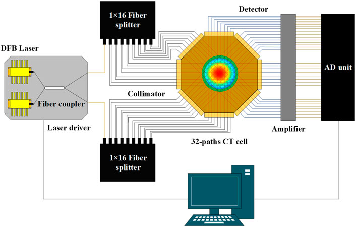
FIGURE 1. CT-TDLAS device connection.

FIGURE 2

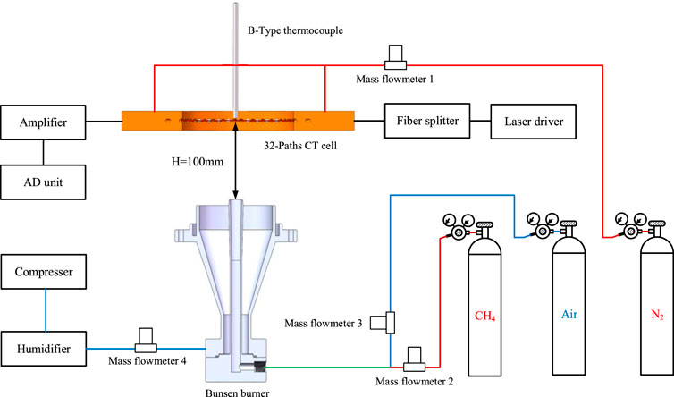
FIGURE 2. CT-TDLAS experiment system.

The flow rates of the Bunsen burner premixed gas consisted of 3.0 L/min methane (CH₄) and 3.0 L/min air. During the combustion process, there was 35 L/min compressed air surrounding the flame to make the premix flame steady. In the CT-TDLAS experiment, the water vapor mainly came from methane combustion. Some researchers usually used flat burner flame to verify the 2D temperature detection performance of the CT-TDLAS technique [15]. In this study, different from the flat burner, the diameter of the Bunsen burner nozzle was 10 mm, and the flame was difficult to fill all the CT measurement areas. Therefore, the H₂O concentration of the laser path located at the CT measurement edge area was extremely inadequate, and H₂O absorption was focused on the laser path that passed through the center area. This phenomenon was harmful to CT reconstruction accuracy. So the compressed air was fed into a humidifier before being inserted into the surrounding area of the Bunsen burner flame.

Before the CT-TDLAS experiment, steady flame combustion must be confirmed. At the center of the CT measurement area, five feature points were established in this study. Feature point 1 was the measurement center point. The other four feature points were, respectively, located at the ±X axis and ±Y axis, and the distance was all 5 mm. During steady flame confirmation, the temperature of five feature points was detected five times by the B-type thermocouple, while the Bunsen burner flame was rekindled 5 min each time. If the temperature was almost the same within confirmation of five times, it can be considered that the flame was in a steady combustion state.

When the flame was confirmed in the steady-combustion state, the B-type thermocouple probe was used to detect the temperature distribution of the center 40 mm × 40 mm area with 121 points, and the distance between each point was 4 mm. After that, the CT-TDLAS system was applied to record the 32-path 1388-nm laser, 1343-nm laser, and coupled laser signal information.

Results and discussion

In this section, the simulate reconstruction accuracy of two represented CT algorithms, SART and Tikhonov regularization, was compared with the performance of the polynomial fitting method. The reconstruction accuracy of the polynomial fitting method was obviously better than that of SART and Tikhonov regularization. SART and Tikhonov regularization had similar reconstruction accuracy, but Tikhonov regularization had an advantage in reconstruction efficiency. Thus, Tikhonov regularization and the polynomial fitting method were applied to the CT-TDLAS reconstruction of the Bunsen burner flame. The thermocouple detection results at the same flame condition were obtained to discuss the actual measurement accuracy of CT-TDLAS with Tikhonov regularization and the polynomial fitting method.

Simulation analysis of CT algorithms’ accuracy

To evaluate the accuracy and efficiency of CT reconstruction with three different CT algorithms, a unimodal and center-symmetric Cauchy–Lorentz temperature distribution was assumed. The assumed area was a 60-mm square. The water vapor concentration was 10%, and the maximum temperature in the center was 1100 K. The expression and image of the temperature distribution are shown in Eq. 16 and Figure 3, respectively. The simulated CT-TDLAS laser path was a 16 × 16 orthogonal structure, as shown in Figure 4. The distance between each laser path was 3.75 mm.

$T=\frac{800\times 13.5^2}{13.5^2+x^2+y^2}+300.(16)$

FIGURE 3

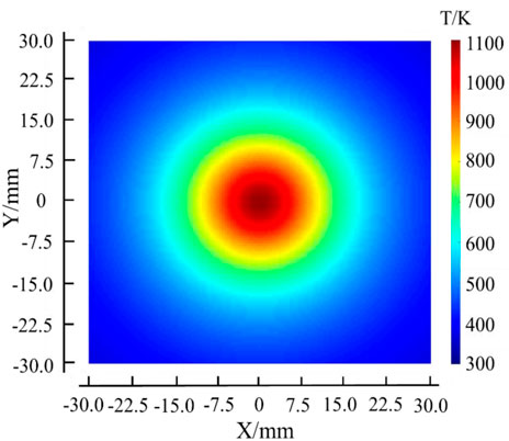
FIGURE 3. Assumed center-symmetric Cauchy–Lorentz temperature distribution.

FIGURE 4

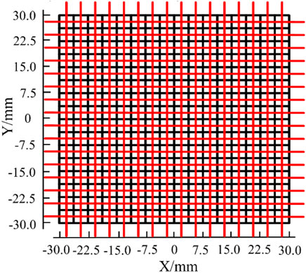
FIGURE 4. 16 × 16 orthogonal simulated laser path structure.

The polynomial fitting method could receive a high-resolution reconstruction result. The CT reconstruction results of SART, Tikhonov regularization, and the polynomial fitting method are shown in Figure 5. The relaxation factor ω used in SART was 0.1, and the initial value of the absorbance used by each optical path during the iteration was set to 0. The resolutions of reconstructed results by SART and Tikhonov regularization were 16 × 16 pixels within a 60-mm square. This resolution was the highest result for these two algorithms to achieve. The reason was that each grid needed at least one laser path to go through. The resolution of the polynomial fitting method was decided by the Taylor expansion series m of the distribution function T (x,y). In this simulate reconstruction, the polynomial fitting method obtained a 39 × 39 pixel resolution result. It was obvious that the polynomial fitting method had an advantage in initial reconstruction resolution. Benefitting from this, integral changes in the temperature gradient could be easily acquired.

FIGURE 5

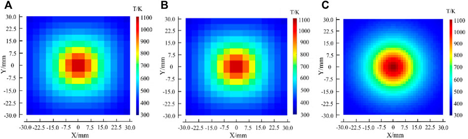
FIGURE 5. CT reconstruction results for assumed temperature distribution. (A) SART algorithm; (B) Tikhonov regularization; and (C) polynomial fitting method.

The polynomial fitting method could receive a more accurate reconstruction result. Because of the central symmetry of the assumed temperature distribution, it was convenient to discuss the accuracy by analyzing the temperature deviation on the path “x = 0 mm”. As shown in Figure 6, the reconstruction results of SART and Tikhonov regularization were almost the same. The mean relative error and maximum relative error of SART were 4.17% and 5.61%, respectively, while the mean relative error and maximum relative error of Tikhonov regularization were 4.22% and 5.58%, respectively. The polynomial fitting method was obviously much closer to the assumed distribution, and the mean relative error and maximum relative error were 1.23% and 1.63%, respectively, because the polynomial fitting method considered more residual terms during the calculation process.

FIGURE 6

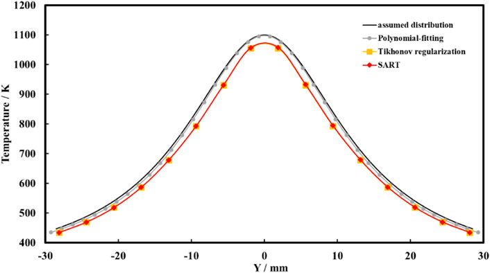
FIGURE 6. Temperature deviation by three CT algorithms on the path “x = 0 mm”.

The polynomial fitting method had the advantage of high resolution and reconstruction accuracy compared with the traditional CT algorithms. It was more suitable for complicated combustion flame detection.

Comparison of CT-TDLAS experimental results using different CT algorithms

According to the previous discussion, SART and Tikhonov regularization could get almost the same accuracy reconstruction results through the orthogonal laser path structure, which was easy to receive an ill-conditioned matrix with the ill-posed solution. However, SART needed a correct each grid absorption value individually during one iterative process, and it costs hours to converge. Tikhonov regularization could quickly get solutions by simple matrix operations. So Tikhonov regularization and the polynomial fitting method were chosen to restructure the Bunsen burn flame.

The polynomial fitting method had significant advantages over actual flame detection. It got a clear and irregular temperature distribution result. In actual flame detection, the 16 × 16 orthogonal laser structure was not satisfied. As shown in Figure 1, the customized 32-path laser structure was divided into four projection directions to reduce the ill-posedness of CT-TDLAS ill-conditioned equations. Tikhonov regularization needed to guarantee that there was at least one laser path going through each grid. So the measurement area of the CT cell was set to a 10 × 10 grid mesh. However, the polynomial fitting method could still get a 39 × 39 pixel result, while the number of laser paths was not changing. The temperature distribution of the Bunsen burner flame has been shown in Figure 7. Because of the resolution limitation, Tikhonov regularization could only get a roughly presented temperature distribution trend. It could not display detailed information such as the gradient change of the flame temperature distribution. The actual combustion was complicated; according to the thermocouple result, the Bunsen burner flame section was not a regular symmetrical appearance, which was related to factors such as the horizontal inclination angle of the fixed Bunsen burner and the premixed gas flow emitted by a nozzle. It would enlarge the deviation when cubic spline interpolation is directly used without any reference to the increasing resolution. The polynomial fitting method could perfectly avoid these problems. In Figure 7C, more accurate and intuitive flame outline messages could be obtained.

FIGURE 7

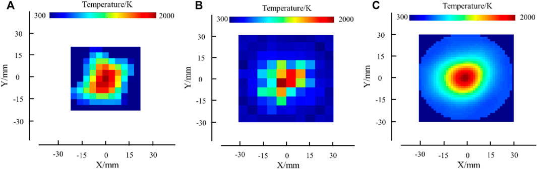
FIGURE 7. Temperature distribution of the Bunsen burner flame. (A) Thermocouple; (B) Tikhonov regularization; and (C) polynomial fitting method.

The accuracy of the polynomial fitting method was convinced in the Bunsen burner flame experiment. The temperature on the path “Y = 0 mm” was compared, as shown in Figure 8. In the range of −10 to 10 mm, combustion was stable at the flame center, so the reconstruction results of the polynomial fitting method were consistent with the thermocouple. However, in the range of −20 to −10 mm and 10–20 mm, there was an obvious deviation between the polynomial fitting method and the thermocouple. In these areas, the unreacted methane gas and the reaction intermediates of the flame all reacted with the oxygen in the surrounding compressed air. The reaction process was complicated in these areas. It was impossible to ensure that the flame was always in the same combustion state during the thermocouple measurement. The constant slight disturbance of the flame would also cause deviation in the thermocouple reading. On the other hand, thermocouples could only collect the heat flux from convection and conduction. The heat radiation would be missed during the detection process. These two factors caused the deviation between the polynomial fitting method and the thermocouple. However, the resolution of the thermocouple measurement results was limited, and the best temperature detection range of the B-type thermocouple was 600–1700°C. In Figure 8, the results of CT-TDLAS with the polynomial fitting method and thermocouple are similar in the temperature range of 900–2000 K. The deviation of flame FWHM and peak temperature position between the polynomial fitting method and thermocouple was acceptable when the effect of calculation and experimental measurement error was considered. The temperature distribution trends of Tikhonov regularization and the polynomial fitting method reconstruction results were consistent, but there was a difference between the measurement center regions. This was due to the insufficient number of pixel grids in Tikhonov regularization.

FIGURE 8

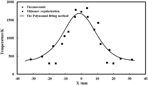
FIGURE 8. Temperature deviation on the path “Y = 0 mm.”

According to the aforementioned comparison results, it could be considered that the polynomial fitting method could accurately reconstruct the two-dimensional temperature distribution of the combustion flame and displayed its temperature gradient change. At the same time, its ability to quickly complete reconstruction calculations had great advantages and potential in the field of industrial online measurement and diagnosis.

Conclusion

This study introduced two common CT algorithms of SART and Tikhonov regularization and proposed a new CT algorithm: the polynomial fitting method. First, compared to the accuracy and efficiency of different CT algorithms by an assumed unimodal and center-symmetric Cauchy–Lorentz temperature distribution and a 16 × 16 orthogonal laser path structure, the comparison results showed that SART and Tikhonov regularization could get almost the same accuracy reconstruction results, while Tikhonov regularization had a much higher computational efficiency. The polynomial fitting method showed more accuracy and higher resolution results. Second, a customized 32-path CT-TDLAS system was built. A Bunsen burner flame temperature distribution with 3.0L/min methane (CH₄) and 3.0 L/min air was reconstructed by the thermocouple, Tikhonov regularization, and the polynomial fitting method. The results exhibited that the polynomial fitting method could display detailed information such as the temperature gradient change, and it could also guarantee the reconstruction accuracy compared to the measured results using the thermocouple. CT-TDLAS with the polynomial fitting method had advantages in accuracy, reconstruction efficiency, resolution, and the adaptability of the laser path arrangement to the actual site environment. It was of great significance in the development of CT-TDLAS combustion diagnosis in practical industrial applications.

Data availability statement

The original contributions presented in the study are included in the article/Supplementary Material; further inquiries can be directed to the corresponding author.

Author contributions

WZ was responsible for all aspects of the study. ZX contributed to the CT-TDLAS experiment. WC was responsible for conceptualization and funding acquisition. ZW was responsible for CT reconstruction calculation and data analysis. DC and JY guided this research, revised, and edited the manuscript.

Conflict of interest

The authors declare that the research was conducted in the absence of any commercial or financial relationships that could be construed as a potential conflict of interest.

Publisher’s note

All claims expressed in this article are solely those of the authors and do not necessarily represent those of their affiliated organizations, or those of the publisher, the editors, and the reviewers. Any product that may be evaluated in this article, or claim that may be made by its manufacturer, is not guaranteed or endorsed by the publisher.

References

1. Radajewski M, Decker S, Krueger L. Direct temperature measurement via thermocouples within an SPS/FAST graphite tool. Measurement (2019) 147:106863. doi:10.1016/j.measurement.2019.106863

CrossRef Full Text | Google Scholar

2. Harada T, Watanabe H, Suzuki Y, Kamata H, Matsushita Y, Aoki H, et al. A numerical investigation of evaporation characteristics of a fuel droplet suspended from a thermocouple. Int J Heat Mass Transfer (2011) 54:649–55. doi:10.1016/j.ijheatmasstransfer.2010.08.021

CrossRef Full Text | Google Scholar

3. Guo LB, Zhang D, Sun LX, Yao SC, Wang ZZ, et al. Development in the application of laser-induced breakdown spectroscopy in recent years: A review. Front Phys (Beijing) (2021) 16(2):22500. doi:10.1007/s11467-020-1007-z

CrossRef Full Text | Google Scholar

4. Boeck LR, Mevel R, Fiala T, Hasslberger J, Sattelmayer T. High-speed OH-PLIF imaging of deflagration-to-detonation transition in H2–air mixtures. Exp Fluids (2016) 57:105. doi:10.1007/s00348-016-2191-z

CrossRef Full Text | Google Scholar

5. Singh S, Musculus MP, Reitz RD. Mixing and flame structures inferred from OH-PLIF for conventional and low-temperature diesel engine combustion. Combustion and Flame (2009) 156:1898–908. doi:10.1016/j.combustflame.2009.07.019

CrossRef Full Text | Google Scholar

6. Ma YF, Lewicki R, Razeghi M, Tittel FK. QEPAS based ppb-level detection of CO and N_2O using a high power CW DFB-QCL. Opt Express (2013) 21(1):1008–1019. doi:10.1364/oe.21.001008

PubMed Abstract | CrossRef Full Text | Google Scholar

7. Qiao SD, Sampaolo A, Patimisco P, Spagnolo V, Ma YF. Ultra-highly sensitive HCl-LITES sensor based on a low-frequency quartz tuning fork and a fiber-coupled multi-pass cell. Photoacoustics (2022) 27:100381. doi:10.1016/j.pacs.2022.100381

PubMed Abstract | CrossRef Full Text | Google Scholar

8. Fu Y, Cao JC, Yamanouchi K, Xu HL. Air-laser-based standoff coherent Raman spectrometer. Ultrafast Sci (2022) 2022:1–9. doi:10.34133/2022/9867028

CrossRef Full Text | Google Scholar

9. Zhang ZH, Zhang FB, Xu B, Xie H, Fu B, Lu X, et al. High-sensitivity gas detection with air-lasing-assisted coherent Raman spectroscopy. Ultrafast Sci (2022) 2022:1–8. doi:10.34133/2022/9761458

CrossRef Full Text | Google Scholar

10. Deng BT, Sima C, Xiao YF, Wang X, Ai Y, Li T, et al. Modified laser scanning technique in wavelength modulation spectroscopy for advanced TDLAS gas sensing. Opt Lasers Eng (2022) 151:106906. doi:10.1016/j.optlaseng.2021.106906

CrossRef Full Text | Google Scholar

11. Weng WB, Larsson J, Bood J, Alden M, Li Z. Quantitative hydrogen chloride detection in combustion environments using tunable diode laser absorption spectroscopy with comprehensive investigation of hot water interference. Appl Spectrosc (2022) 76(2):207–15. doi:10.1177/00037028211060866

PubMed Abstract | CrossRef Full Text | Google Scholar

12. Yang XY, Peng ZM, Ding YJ, Du Y. Temperature and OH concentration measurements by ultraviolet broadband absorption of OH(X) in laminar methane/air premixed flames. Fuel (2021) 288:119666. doi:10.1016/j.fuel.2020.119666

CrossRef Full Text | Google Scholar

13. Liu XN, Ma YF. Tunable diode laser absorption spectroscopy based temperature measurement with a single diode laser near 1.4 μm. Sensors (2022) 22:6095. doi:10.3390/s22166095

PubMed Abstract | CrossRef Full Text | Google Scholar

14. Liang TT, Qiao SD, Liu X, Ma YF. Highly sensitive hydrogen sensing based on tunable diode laser absorption spectroscopy with a 2.1 μm diode laser. Chemosensors (2022) 10:321. doi:10.3390/chemosensors10080321

CrossRef Full Text | Google Scholar

15. Sun PS, Zhang ZR, Li Z, Guo Q, Dong F. A study of two dimensional tomography reconstruction of temperature and gas concentration in a combustion field using TDLAS. Appl Sci (Basel) (2017) 7(10):990. doi:10.3390/app7100990

CrossRef Full Text | Google Scholar

16. Xia HH, Kan RF, Liu JG, Xu ZY, He YB. Analysis of algebraic reconstruction technique for accurate imaging of gas temperature and concentration based on tunable diode laser absorption spectroscopy. Chin Phys B (2016) 25(6):064205. doi:10.1088/1674-1056/25/6/064205

CrossRef Full Text | Google Scholar

17. Liu C, Xu LJ, Chen JL, Cao Z, Lin Y, Cai W. Development of a fan-beam TDLAS-based tomographic sensor for rapid imaging of temperature and gas concentration. Opt Express (2015) 23(17):22494. doi:10.1364/oe.23.022494

PubMed Abstract | CrossRef Full Text | Google Scholar

18. Kamimoto T, Deguchi Y, Zhang N, Nakao R, Takagi T, Zhang JZ. Real-time 2D concentration measurement of CH4 in oscillating flames using CT tunable diode laser absorption spectroscopy. J Appl Nonlinear Dyn (2015) 4(3):295–303. doi:10.5890/jand.2015.09.009

CrossRef Full Text | Google Scholar

19. Deguchi Y, Kamimoto T, Kiyota Y. Time resolved 2D concentration and temperature measurement using CT tunable laser absorption spectroscopy. Flow Meas Instrumentation (2015) 46:312–8. doi:10.1016/j.flowmeasinst.2015.06.025

CrossRef Full Text | Google Scholar

20. Wang ZZ, Zhou WZ, Kamimoto T, Deguchi Y, Yan J, Yao S, et al. Two-dimensional temperature measurement in a high-temperature and high-pressure combustor using computed tomography tunable diode laser absorption spectroscopy (CT-TDLAS) with a wide-scanning laser at 1335–1375 nm. Appl Spectrosc (2020) 14(2):210–22. doi:10.1177/0003702819888214

CrossRef Full Text | Google Scholar

21. Xia HH, Kan RF, Xu ZY, Liu J, He Y, Yang C, et al. Measurements of axisymmetric temperature and H₂O concentration distributions on a circular flat flame burner based on tunable diode laser absorption tomography. In: International Symposium on Hyperspectral Remote Sensing Applications/International Symposium on Environmental Monitoring and Safety Testing Technology; 9-11 May 2016; Beijing, China. Proc.SPIE (2016). p. 10156.

Google Scholar

22. Han Y, Ye JC. Framing U-net via deep convolutional framelets: Application to sparse-view CT. IEEE Trans Med Imaging (2018) 37:1418–29. doi:10.1109/tmi.2018.2823768

PubMed Abstract | CrossRef Full Text | Google Scholar

23. Choo JY, Goo JM, Lee CH, Park CM, Park SJ, Shim MS. Quantitative analysis of emphysema and airway measurements according to iterative reconstruction algorithms: Comparison of filtered back projection, adaptive statistical iterative reconstruction and model-based iterative reconstruction. Eur Radiol (2014) 24(4):799–806. doi:10.1007/s00330-013-3078-5

PubMed Abstract | CrossRef Full Text | Google Scholar

24. Zhang GY, Wang GQ, Huang Y, Liu X. Reconstruction and simulation of temperature and CO2 concentration in an axisymmetric flame based on TDLAS. Optik (2018) 170:166–77. doi:10.1016/j.ijleo.2018.05.123

CrossRef Full Text | Google Scholar

25. Guha A, Schoegl I. Tomographic laser absorption spectroscopy using Tikhonov regularization. Appl Opt (2015) 53(34):8095–8103. doi:10.1364/ao.53.008095

PubMed Abstract | CrossRef Full Text | Google Scholar

26. Choi DW, Jeon MG, Cho GR, Kamimoto T, Deguchi Y, Doh DH. Performance improvements in temperature reconstructions of 2-D tunable diode laser absorption spectroscopy (TDLAS). J Therm Sci (2016) 25(1):84–9. doi:10.1007/s11630-016-0837-z

CrossRef Full Text | Google Scholar

27. Peng D, Jin Y, Zhai C, Yang J. Numerical simulations to improve the performance of tunable diode laser absorption tomography in a harsh combustion environment. Spectrosc Lett (2018) 51(1):7–16. doi:10.1080/00387010.2017.1399424

CrossRef Full Text | Google Scholar

28. Shao J, Wang LM, Ying CF. Numerical investigation of the two-dimensional gas temperature distribution based on tunable diode laser absorption spectroscopy. Optica Applicata (2015) 45(2):183–198. doi:10.5277/oa150205

CrossRef Full Text | Google Scholar

29. Busa KM, McDaniel JC, Brown MS. Implementation of maximum-likelihood expectation-maximization algorithm for tomographic reconstruction of TDLAT measurements. In: 52nd AIAA Aerospace Sciences Meeting; 2014, January 13-17; National Harbor, MD, USA. American Institute of Aeronautics and Astronautics (2014). p. 1–15.

CrossRef Full Text | Google Scholar

30. Nadir Z, Brown MS, Comer ML, Bouman CA. A model-based iterative reconstruction approach to tunable diode laser absorption tomography. IEEE Trans Comput Imaging (2017) 3(4):876–90. doi:10.1109/tci.2017.2690143

CrossRef Full Text | Google Scholar

31. Si J, Fu G, Zhang R, Rui Z, Godwin E, Liu C, et al. A quality-hierarchical temperature imaging network for TDLAS tomography. IEEE Transcations Instrumentation Meas (2022) 71:4500710. doi:10.1109/TIM.2022.3144211

CrossRef Full Text | Google Scholar

32. Huang A, Cao Z, Wang CR, Wen J, Lu F, Xu L. An FPGA-based on-chip neural network for TDLAS tomography in dynamic flames. IEEE Trans Instrum Meas (2021) 70:4506911–11. doi:10.1109/tim.2021.3115210

CrossRef Full Text | Google Scholar

33. Chen P, Kan LL, Song XM, Wang X, Jiang C. Application of VMD and Mahalanobis distance combination algorithm in TDLAS methane gas detection. Optik (2021) 728:166114. doi:10.1016/j.ijleo.2020.166114

CrossRef Full Text | Google Scholar

34. Zhang S, Xia YS, Zou CZ. An adaptive regularization method for low-dose CT reconstruction from CT transmission data in Poisson-Gaussian noise. Optik (2019) 188:172–86. doi:10.1016/j.ijleo.2019.04.005

CrossRef Full Text | Google Scholar

35. Gonzales B, Lalush D. Full-spectrum CT reconstruction using a weighted least squares algorithm with an energy-Axis penalty. IEEE Trans Med Imaging (2011) 30(2):173–83. doi:10.1109/tmi.2010.2048120

PubMed Abstract | CrossRef Full Text | Google Scholar

36. Liu C, Xu LJ, Cao Z. Measurement of nonuniform temperature and concentration distributions by combining line-of-sight tunable diode laser absorption spectroscopy with regularization methods. Appl Opt (2013) 52(20):4827–4842. doi:10.1364/ao.52.004827

PubMed Abstract | CrossRef Full Text | Google Scholar

37. Cai WW, Kaminski CF. Multiplexed absorption tomography with calibration-free wavelength modulation spectroscopy. Appl Phys Lett (2014) 104(15):154106. doi:10.1063/1.4871976

CrossRef Full Text | Google Scholar

38. Ma L, Cai WW, Caswell AW, Kraetschmer T, Sanders ST, Roy S, et al. Tomographic imaging of temperature and chemical species based on hyperspectral absorption spectroscopy. Opt Express (2009) 17(10):8602–8613. doi:10.1364/oe.17.008602

PubMed Abstract | CrossRef Full Text | Google Scholar