 Haikang He
 Baojiang Sun1*
 Xuefeng Li
95% of researchers rate our articles as excellent or good
Learn more about the work of our research integrity team to safeguard the quality of each article we publish.
Find out more
ORIGINAL RESEARCH article
Front. Phys. , 07 October 2022
Sec. Interdisciplinary Physics
Volume 10 - 2022 | https://doi.org/10.3389/fphy.2022.1028671
This article is part of the Research Topic Multiphase Flow Behavior in the Deep-Stratum and Deep-Water Wellbores View all 13 articles
The dissolution of invaded gas in the drilling fluid during drilling results in an increase in the gas invasion concealment. This is of great significance for the development of acid gas reservoirs to determine the solubility change and multiphase flow law in an annulus after invasion by natural gas with high CO2 content. In this study, control equations of gas–liquid flow during drilling gas invasion are established considering the influence of gas solubility. For the prediction of gas solubility, the interaction parameters of CH4 and water in the Peng–Robinson equation of state are optimised to establish a gas solubility prediction model. The solubility of natural gas with high CO2 content in water and brine solution is measured through phase-equilibrium experiments. The results indicate that the newly optimised solubility model can accurately predict the solubility of CH4 and CO2 in water, and the prediction error is within 5%. Moreover, the prediction error for the solubility of CH4 and CO2 mixed gas is within 15%. The analysis of gas invasion in example engineering drilling applications reveals that an increase in the CO2 content in the invaded gas leads to a slow change in the mud-pit increment, and the concealment strengthens as the distance between the gas-migration front and the wellhead increases. Gas solubility has a significant impact on the monitoring of gas invasion in low permeability reservoirs.
The Liwan 3-1 gas field in China, with CH4 content exceeding 80% and CO2 content exceeding 3%, is a type of acidic gas field [1–7]. Romania, Mexico, and Indonesia have gas reservoirs with high CO2 content, that is, the CO2 concentration in the reservoir fluid is as high as 86% [8–10], and the CO2 content in the natural gas produced at the Tugu Barat oilfield in Indonesia is as high as 76 mol% [11]. During the drilling and development of natural gas fields containing CO2, formation fluid invasion can easily occur. A high amount of invaded gas dissolution in the drilling fluid makes it difficult to monitor the ground and increases the blowout risk. Several studies have focused on the law of gas dissolution in multiphase flow. For example, Yin et al. (2017) established an annular multiphase transient flow model based on gas–liquid two-phase flow and flash theory, considering the dissolution of gas in an oil-based drilling fluid. The dissolution of gas led to a slow change of mud pit, and the mud pit increment associated with the oil-based drilling fluid was smaller than that of the water-based drilling fluid [12]. Sun et al. (2018) considered the phase change and dissolution of the acidic natural mixture in a drilling fluid and proposed a flow-transition criterion for multiphase flow. When the invading gas rises in a vertical wellbore, the gas phase change causes large volume expansion and increases the blowout risk. However, they focused on the gas phase state analysis and did not consider the gas dissolution effect [13]. Xu et al. (2018) used the standing bubble point formula to calculate the solubility of gas in oil. Neglecting the gas dissolution effect, the bottom-hole temperature was overestimated by 3.74°C, and the bottom-hole pressure increased by 2.92 MPa [14].
The O’Bryan formula [15] is widely used to predict the solubility of gas in an oil-based drilling fluid. A water-based drilling fluid system is mainly composed of water and salt; therefore, the solubility of water-based drilling fluids is typically studied using water and salt water. Wiebe and Gaddy (1939), Briones et al. (1987), and Sabirzyanov et al. (2003) conducted a large number of experimental studies on the solubility of CO2 gas in water [16–18]. It was found that the temperature could be as high as 373.15 K and the pressure could reach 70 MPa. However, studies on the solubility of a mixture of CH4 and CO2 in water and salt water remain limited. Dhima (1999) measured the solubility of CO2 + CH4 mixture in water at 344.5 K and 10–100 MPa [19]. Subsequently, Qin et al. (2008), Ghafri (2014), and Loring et al. (2017) obtained the vapour–liquid equilibrium data for the CO2 + CH4 + H2O ternary system at 323.15–423.15 K and 1–20 MPa [20–22]. Zirrahi et al. [23] recalculated the mutual parameters between gases in the Peng–Robinson equation of state (PR-EOS) [24] using existing experimental data for mixed gas solubility. The prediction deviation of the solubility of the acidic mixed gas in water was less than 5%; however, the applicability must be evaluated based on the adjustment of the fitting parameters of the experimental data. Ziabakhsh-Ganji and Kooi [25] improved the state equation to establish a gas solubility prediction model. Although the model could accurately predict the solubility of single gas in water and brine, the prediction accuracy of the solubility of mixed gases remains unknown. Li [26] predicted the phase equilibrium of CO2–CH4–H2S–brine using fugacity-fugacity and fugacity-activity models and found that the fugacity-activity model was more accurate in predicting the solubility of CO2 + CH4 mixed gas.
Research on the effect of gas dissolution on multiphase flow has focused on oil-based drilling fluids, and water-based drilling fluids have typically been neglected because of the low solubility of gases in water. Furthermore, the accuracy and applicability of existing prediction models are insufficient for determining the water solubility of a mixed gas containing CO2. Therefore, according to the characteristics of deep-water drilling, a gas–liquid two-phase flow control model incorporating the gas dissolution effect was established in this study. To realise accurate prediction and analysis of gas solubility, the interaction parameters of CH4 and water in the PR-EOS were optimised to establish a gas solubility prediction model. The finite difference method was used to solve the proposed multiphase flow model. The influence of gas solubility on gas phase flow law during gas invasion was analysed using an example to provide guidance for the control safety of field wells.
According to the law of mass conservation, a physical model of continuity, momentum, and energy was established by considering the dissolution of gas in a drilling fluid based on the following assumptions.
1) The flow in the wellbore is one-dimensional.
2) The dissolution of gas in the drilling fluid is completed instantaneously.
3) The compressibility change of drilling fluid is negligible.
4) The influence of rock debris can be neglected.
The continuity equation for the free gas phase can be expressed as follows:
where mg-L is the mass transfer rate from gas phase to liquid phase [kg/(m s)], which can be expressed as
The mass conservation of the liquid phase can be expressed as
Considering the slippage of the gas–liquid phase, the momentum equation of the gas–liquid phase can be expressed as
Latent heat of phase change exists during the process of gas–liquid phase equilibrium. Considering the existence of heat associated with phase change, the energy equation of the annulus in a wellbore is expressed as follows.
Gas phase:
Liquid phase:
Phase-change heat:
Therefore, the energy equation in the wellbore annulus can be expressed as
Sun et al. applied the power-law for fluid flow to liquid phase flow [27] to obtain the following equation:
When Re < 2,000,
When Re > 2,000,
Bubbly flow:
Slug and churn flows:
Annular fog flow:
The occurrence of gas kicks in deep-water drilling wellbores induces multiphase flow in the wellbore as well as gas inflow from the reservoir, which are influenced by each other. For example, when the wellbore pressure is lower than the pore pressure of the open-hole section, a gas surge occurs. Subsequently, once the gas enters the wellbore, the flow rate, gas porosity, and fluid pressure change. The gas inflow can be calculated using the following [28]
PR-EOS was used for calculating the physical properties of the fluid components in the wellbore. The auxiliary equations such as velocity and two-phase flow-state discrimination equations were obtained from Gao et al. [29].
The gas–liquid two-phase equilibrium in a closed system can be expressed as follows:
PR-EOS was used for calculating the fugacity coefficients of component i in the gas and liquid phases, and its basic form can be expressed as follows:
For a single gas, the parameters a and b are
A non-random mixing rule was used for calculating the mixed gas parameters a and b, as follows:
where kij is the interaction parameter between i and j components, with kij = kji. For calculating the fugacity coefficients, combined with van der Waals mixing rule [30], the following expression was used:
The compression factor is calculated as
where the parameters A and B are functions of temperature and pressure and are expressed as follows:
The binary interaction parameter in PR-EOS reflects the nature of the interaction between two molecules in a mixed system of gas and water and is the key parameter for obtaining an accurate prediction of phase equilibrium using PR-EOS. Interaction parameters are typically determined based on the optimised regression of the experimental data for gas–liquid phase equilibrium. There are several reports on the solubility of CH4 in water, and the data incorporated in this study are presented in the Appendix. The interaction parameters were calculated at different temperatures and pressures (see Figure 1). Evidently, the interaction parameters increase with an increase in temperature, whereas they exhibit a decreasing trend with an increase in pressure; however, the fluctuation range is not significantly affected by temperature. The interaction parameters were fitted as a function of temperature and pressure, as follows:
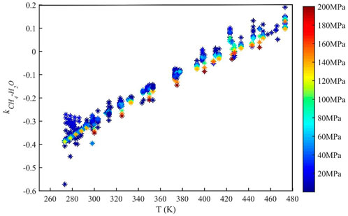
FIGURE 1. Variation in the interaction parameters of CH4 and water with temperature and pressure.
To verify the applicability of the gas solubility prediction model established by optimising the parameters of PR-EOS, the solubility of CO2, CH4, and CO2 + CH4 mixed gas in water was measured using a phase-equilibrium experimental device. The accuracy of the model prediction was expressed by the average relative deviation percentage ARD%, and average absolute relative deviation AARD%.
The purity of CO2 and CH4 was greater than 99.9%, and the purity of CH4 in the CO2 + CH4 mixed gas was greater than 49.9%. Figure 2 shows the experimental flow diagram. The high-temperature and high-pressure reactor used had a volume of 300 ml, with a maximum pressure and temperature resistance of 60 MPa and 473 K, respectively. A constant-speed and constant-pressure pump (D-250L) was used for pressurisation, with a maximum pressure of 70 MPa.
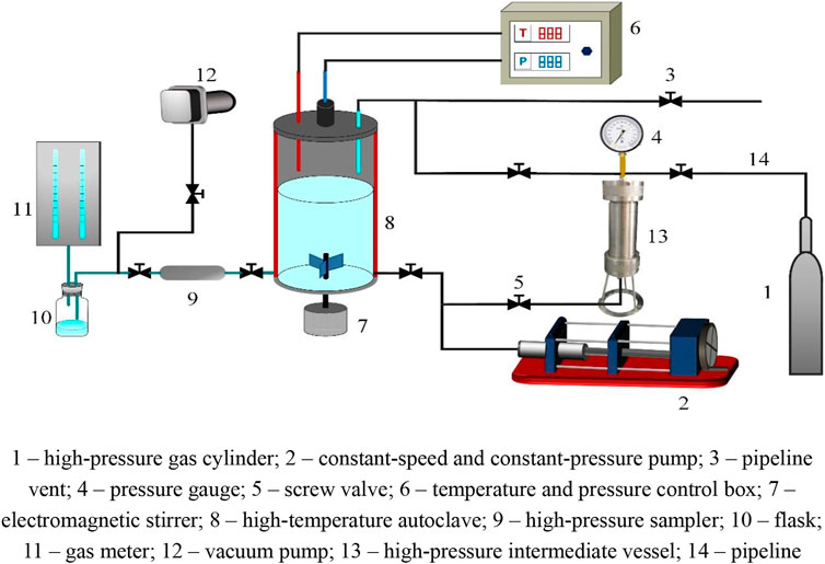
FIGURE 2. Schematic of the experimental flow.
The operational process for gas solubility measurement is as follows.
1) The experimental device is cleaned and checked for air tightness. Deionized water is used to clean the high-temperature and high-pressure reaction kettle 2–3 times; the intermediate vessel and reaction kettle are connected; the pressure of the reaction kettle is increased to 5 MPa. If the pressure of the reaction kettle and intermediate vessel is stable without fluctuation within 2 h, the sealing of the experimental device is considered adequate. Otherwise, the connection is rechecked.
2) The phase-equilibrium experiment is conducted by pressurising and heating. A vacuum is generated in the reaction kettle using a vacuum pump. Approximately 200 ml of liquid is injected with a constant-speed and constant-pressure pump, and the heating device is turned on to increase the temperature to the pre-set value. The reaction kettle is filled with gas to a certain pre-set pressure through the intermediate vessel to form a gas–liquid mixed state in the kettle. During the pressurisation process, certain temperature fluctuations occur because of the adiabatic condition in the reaction kettle; therefore, the temperature must be stabilised to the pre-set temperature. After stirring for 1–2 h with an electromagnetic stirrer, the pressure change in the kettle is no longer monitored. If the pressure is stable within 2–3 h, the gas–liquid equilibrium is considered stable.
3) The measurement data is recorded, sampled, and analysed. A vacuum pump is used to generate a vacuum in the sampler and extract the liquid in the kettle. A constant-speed and constant-pressure pump is used to inject the liquid into the reaction kettle and maintain a stable pressure in the kettle. A gas meter is used to measure the volume of the precipitated gas. After the gas is collected, the gas and liquid volumes are recorded in real-time. The average value of the three measurements is calculated and chromatographic analysis of the precipitated gas is performed.
4) Steps 2)–3) are repeated to perform the solubility measurements at different pressures and temperatures. After the experiment is completed, the exhaust pipeline is vented.
To verify that the aforementioned experimental devices and methods can be used for solubility measurements, the measurement results of CO2 gas at 325.15 K were compared with previously reported experimental data [18, 20, 31], as presented in Table 1. Evidently, the maximum ARD% of our experimental data compared with reported data is 3.54, and the minimum ARD% is 1.55, indicating good accuracy. Therefore, the proposed experimental apparatus and method can be used for gas solubility measurements.
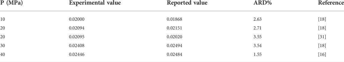
TABLE 1. Comparison between experimental and previously reported values of CO2 solubility in water measured at 323.15 K.
Solubility of CH4 and CO2 in water at 323.15 K was measured using the proposed experimental device. The developed solubility-prediction model was used to predict and analyse the solubility of CO2 and CH4 in water, as shown in Figures 3, 4. The experimental data obtained in this study were compared with previously reported data [16–18, 32–35] for model analysis.
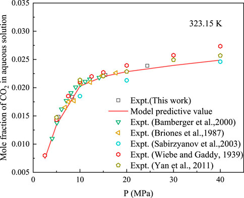
FIGURE 3. Comparison between predicted data of CO2 solubility model and experimental data at 323.15 K.
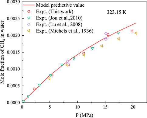
FIGURE 4. Comparison between predicted data of CH4 solubility model and experimental data at 323.15 K.
At 323.15 K, the AARD% of the model predicted and experimental values for CH4 was 5.66, and the AARD% for the solubility of CO2 in water was 3.71. Therefore, the proposed solubility-prediction model can be used to accurately predict the solubility of CH4 and CO2.
The solubility of the CH4 + CO2 mixture in water and 5% NaCl aqueous solution was measured at 302.15 K and 323.15 K. The established solubility model was used to predict the experimental results, as shown in Figure 5. Evidently, the model predicted values are not consistent with the experimental values and a certain deviation exists. For the solubility of the mixture in water, the AARD% of the model predicted and experimental values was 14.80. The AARD% of the mixed gas in 5% NaCl was 14.32, showing a certain deviation. This is because this study only investigated the interaction parameters of CH4 gas and water. The interaction parameters of CO2–H2O are 0.19014, as reported by Ziabakhsh-Ganji and Kooi [25], and the interaction parameters of CO2–CH4 are 0.1 [36]. Therefore, the selection of interaction parameters resulted in a lower model predicted value for CO2.
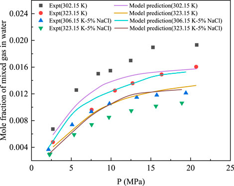
FIGURE 5. Comparison between the predicted data of CH4 solubility model and the experimental data at 323.15 K.
The finite difference method was used to calculate the differences in the proposed multiphase flow model [37]. The basic difference calculation can be expressed as follows:
The discretisation of the differential equation describing the gas phase non-production interval can be expressed as follows:
The discretisation of the differential equation of the dissolved phase can be expressed as follows:
The phase discretisation of the drilling fluid differential equation can be expressed as follows:
The momentum equation discretisation can be expressed as follows:
The flow diagram of the solution process in the proposed model is illustrated in Figure 6. The specific steps of the multiphase flow model are as follows.
1) The bottom-hole pressure
2) The dissolved gas at node j and time n is calculated. The relationship between the calculated gas dissolution and the formation-gas inflow or production is examined, as follows.
① If the calculated gas dissolution is less than the gas inflow, the gas dissolution at the current time is the calculated gas solubility.
② If the calculated gas dissolution is greater than the gas inflow, the gas dissolution at the current time is the inflow of formation gas.
3) According to the calculated temperature and pressure at node j at time n, output of each phase, and dissolved amount of gas, the physical property parameters of each component phase at node j and time n are calculated using the equation of state.
4) The continuity equation is used to calculate the velocity and volume fraction
5) The pressure
6) Steps 2)–5) are repeated to calculate the wellhead parameters, and the calculated wellhead back pressure is
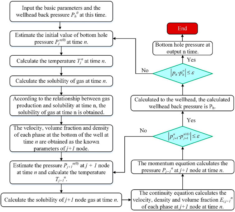
FIGURE 6. Flowchart of multiphase flow model solution.
A deep-water vertical well in the South China Sea was used as an example to perform a project case analysis. The basic data are listed in Table 2.
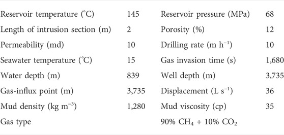
TABLE 2. Specifications of the example well.
Figure 7 shows the deviation between the calculated mud-pit increment and the measured values. It can be observed that the mud-pit increment rapidly changes in the range of 0–210 s. Furthermore, the difference between the calculated curve and the measured points is small, and the error between the predicted and the measured values remains within 15%. In actual engineering projects involving drilling, the measured data fluctuates owing to the influence of tide, instrument error, and typhoon.
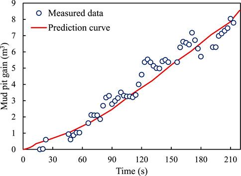
FIGURE 7. Variation in the relationship between mud-pit increment and bottom-hole pressure with invasion time.
Figures 8, 9 show the variation in the relationship between the volume fraction of the free gas and the mass fraction of the dissolved gas with invasion time. As the well depth decreases, both the mass fraction of the dissolved gas and the corresponding free gas integral number gradually decrease. This is because the amount of gas invaded by the formation is limited, and the gas gradually extends to the front. The gas dissolution causes the volume fraction of the gas at the front to decrease. However, when the well depth is fixed, volume fraction of the free gas increases with an increase in invasion time, primarily because the amount of dissolved gas in the drilling fluid reaches the saturated state, and the amount of gas released increases. As is evident from Figure 9, the dissolved gas content in the wellbore has a certain limit and does not increase beyond the liquid saturation value.
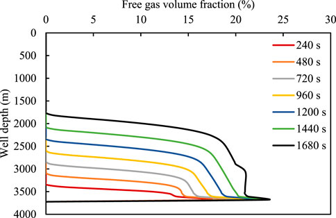
FIGURE 8. Relationship between free gas integral number and well depth for different time durations.
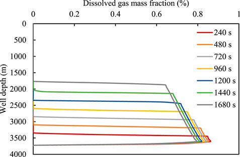
FIGURE 9. Relationship between dissolved gas mass fraction and well depth.
The gas–liquid two-phase flow law was simulated and analysed for a reservoir permeability of 10 md, gas invasion time of 1,200 s, and displacement of 36 L/s. Figure 10 shows the variations in the mud-pit increment with gas invasion time under different acid gas contents and permeabilities. If the invaded gas does not contain CO2, the mud pit changes rapidly and the gas invasion monitoring time is shorter. By contrast, if the invaded gas contains a high concentration of CO2, the incremental change time of the mud pit increases. If the monitoring value of the mud-pit increment is considered as 10 m3, it can be monitored in 252 s when the gas without CO2 is dissolved. When 10% CO2 is present in the invading gas, the monitoring time of gas invasion increases by 10 s. Similarly, the monitoring time of the gas containing 20% CO2 is increased by 22 s. Therefore, the dissolution of an acid gas causes a certain lag and increased risk in gas invasion monitoring. For the 90% CH4 + 10% CO2 intrusive gas, the monitoring time changes in mud pits with different permeabilities. With an increase in invasion time, the mud-pit increment changes rapidly under high permeability. If 5 m3 is used as the monitoring standard, the time required to attain the monitoring value under high permeability is shorter. This is because an increase in gas invasion under high permeability results in an increase in gas content in the wellbore.
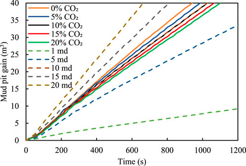
FIGURE 10. Variation in the mud pit increment with time for different gas types and permeabilities.
Figures 11, 12 show the relationship between the volume fraction of the free gas and the mass fraction of the dissolved gas for different acid gas contents and well depths. Evidently, the number of free gas integrals decreases and the corresponding dissolved gas content increases with an increase in the CO2 content. This is because an increase in the acid gas content leads to a rapid increase in the amount of dissolved gas in the drilling fluid; consequently, more gas enters the drilling fluid, resulting in a decrease in the number of free gas integrals.
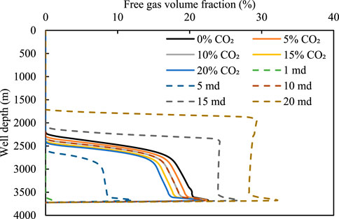
FIGURE 11. Variation in the free gas integral number with well depth for different intrusive gases and permeabilities.
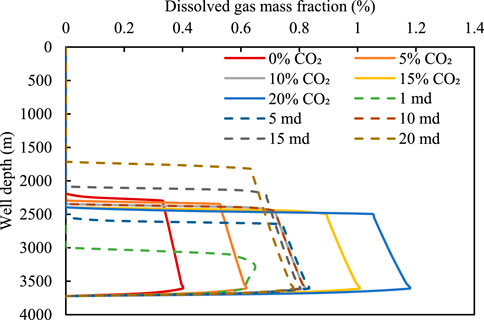
FIGURE 12. Relationship between mass fraction of dissolved gas and well depth for different intrusive gases and permeabilities.
For the 90% CH4 + 10% CO2 intrusive gas, the changes in the free gas and dissolved gas under different reservoir permeabilities are examined. Under a low permeability of 1 md, the amount of invading gas is small. Therefore, the gas is completely dissolved in the drilling fluid, causing the integral number of free gas to be 0 (see Figure 11). With an increase in permeability, the amount of invading gas in the wellbore increases, because the solubility of the gas in the drilling fluid is limited. The integral number of free gas increases gradually with an increase in permeability, and the position of the gas movement front is closer to the wellhead. Therefore, the dissolution of gases makes timely detection of gas invasion under low permeability difficult; therefore, the concealment is enhanced.
In this study, a multiphase flow model considering gas dissolution was established, and the auxiliary equations of gas solubility were examined based on the dynamic analysis of the migration process of an acid gas invading a wellbore. The main conclusion are as follows.
1) By optimising the interaction parameters of CH4 and water, a new solubility model was established. The prediction accuracy of CH4 gas solubility was maintained at 96.4%. However, the prediction error for the mixed gas composed of CO2 and CH4 was large, and the accuracy was less than 85%.
2) The higher the CO2 content in the invading gas, the greater the amount of dissolved gas in the drilling fluid, the lower the volume fraction of the free gas phase in the wellbore, and the farther the gas front was from the wellhead. Furthermore, the dissolution of gas with high CO2 content caused an increase in the time required for the mud pit increment to reach the warning or critical value.
3) The greater the permeability of the reservoir, the smaller the influence of gas dissolution. For a low permeability reservoir, the influence of gas dissolution plays a key role, resulting in a slow change in the free gas integral number in the wellbore. Moreover, the ground monitoring time was significantly increased, making gas invasion monitoring challenging.
The original contributions presented in the study are included in the article/supplementary material, further inquiries can be directed to the corresponding author.
HH: Methodology, Writing—Original draft preparation. BS: Conceptualization, Supervision, Funding acquisition. XS: Validation, Data curation, Funding acquisition. XL: Data curation. ZS: Data curation.
The author sincerely thanks the Postdoctoral innovative talents support program in China (BX2021374), and the National Natural Science Foundation—Youth Foundation (5210040269) to provide fund support.
Author ZS was employed by the company Drilling Division of China Petroleum Offshore Engineering Co., Ltd.
The remaining authors declare that the research was conducted in the absence of any commercial or financial relationships that could be construed as a potential conflict of interest.
All claims expressed in this article are solely those of the authors and do not necessarily represent those of their affiliated organizations, or those of the publisher, the editors and the reviewers. Any product that may be evaluated in this article, or claim that may be made by its manufacturer, is not guaranteed or endorsed by the publisher.
1. Gao G, Gang W, Zhang G, He W, Cui X, Shen H, et al. Physical simulation of gas reservoir formation in the Liwan 3-1 deep-water gas field in the Baiyun sag, Pearl River Mouth Basin. Nat Gas Industry B (2015) 2(1):77–87. doi:10.1016/j.ngib.2015.02.006
2. Zhang G, Wang D, Lan L, Liu S, Su L, Wang L, et al. The geological characteristics of the large- and medium-sized gas fields in the South China Sea. Acta Oceanol Sin (2021) 40(2):1–12. doi:10.1007/s13131-021-1754-x
3. Zhu W, Huang B, Mi L, Wilkins RWT, Fu N, Xiao X. Geochemistry, origin, and deep-water exploration potential of natural gases in the Pearl River Mouth and Qiongdongnan basins, South China Sea. Am Assoc Pet Geol Bull (2009) 93(6):741–61. doi:10.1306/02170908099
4. Sun BJ, Fu WQ, Wang N, Wang ZY, Gao YH. Multiphase flow modeling of gas intrusion in oil-based drilling mud. J Pet Sci Eng (2019) 174:1142–51. doi:10.1016/j.petrol.2018.12.018
5. Chen B, Sun H, Zhou H, Yang M, Wang D. Effects of pressure and sea water flow on natural gas hydrate production characteristics in marine sediment. Appl Energ (2019) 238:274–83. doi:10.1016/j.apenergy.2019.01.095
6. Chen B, Sun H, Zheng J, Yang M New insights on water-gas flow and hydrate decomposition behaviors in natural gas hydrates deposits with various saturations[J]. Appl. Energy (2020) 259:114185.
7. Sun H, Chen B, Pang W, Song Y, Yang M. Investigation on plugging prediction of multiphase flow in natural gas hydrate sediment with different field scales. Fuel (2022) 325:124936. doi:10.1016/j.fuel.2022.124936
8. Fu WQ, Wang ZY, Sun BJ, Xu JC, Chen LT, Wang XR. Rheological properties of methane hydrate slurry in the presence of xanthan gum. SPE J (2020) 25(5):2341–52. doi:10.2118/199903-pa
9. Fu WQ, Wang ZY, Chen LT, Sun BJ. Experimental investigation of methane hydrate formation in the carboxmethylcellulose (CMC) aqueous solution. SPE J (2020) 25(3):1042–56. doi:10.2118/199367-pa
10. Popp VV, Marinescu M, Manoiu D, Popp A, Chitu PM “Possibilities of energy recovery from CO2 reservoirs[C],” in SPE Annual Technical Conference and Exhibition (OnePetro) (1998).
11. Prakasa Y, Hartanto E, Sulistyo D. United nations conference of plenipotentiaries on a supplementary convention on the abolition of slavery, the slave trade, and institutions and practices similar to slavery (1998).Carbon dioxide generation in Tugu Barat-C field and role in hydrocarbon migration
12. Yin B, Liu G, Li X. Multiphase transient flow model in wellbore annuli during gas kick in deepwater drilling based on oil-based mud. Appl Math Model (2017) 51(11):159–98. doi:10.1016/j.apm.2017.06.029
13. Sun B, Guo Y, Sun W, Gao Y, Li H, Wang Z, et al. Multiphase flow behavior for acid-gas mixture and drilling fluid flow in vertical wellbore[J]. J Pet Sci Eng (2018) 165:388–396. doi:10.1016/j.petrol.2018.02.016
14. Xu Z, Song X, Li G, Zhu Z, Zhu B Gas kick simulation in oil-based drilling fluids with the gas solubility effect during high-temperature and high-pressure well drilling[J]. Appl Therm Eng (2019) 149:1080–1097.
15. O'bryan PL. Well control problems associated with gas solubility in oil-based drilling fluids [D]. Louisiana: Louisiana State University (1988).
16. Wiebe R, Gaddy VL. The solubility in water of carbon dioxide at 50, 75 and 100°, at pressures to 700 atmospheres. J Am Chem Soc (1939) 61(2):315–8. doi:10.1021/ja01871a025
17. Briones JA, Mullins JC, Thies MC, Kim BU. Ternary phase equilibria for acetic acid-water mixtures with supercritical carbon dioxide. Fluid Phase Equilibria (1987) 36(2):235–46. doi:10.1016/0378-3812(87)85026-4
18. Sabirzyanov AN, Shagiakhmetov RA, Gabitov FR, Tarzimanov AA, Gumerov FM. Water solubility of carbon dioxide under supercritical and subcritical conditions[J]. Theor Foundations Chem Eng (2003) 37(1):51–3. doi:10.1023/a:1022256927236
19. Dhima A, De Hemptinne JC, Jose J. Solubility of hydrocarbons and CO2 mixtures in water under high pressure[J]. Ind Eng Chem Res (1999) 38(8):3144–61. doi:10.1021/ie980768g
20. Qin J, Rosenbauer RJ, Duan Z. Experimental measurements of vapor–liquid equilibria of the H2O + CO2 + CH4 ternary system. J Chem Eng Data (2009) 53(6):1246–9. doi:10.1021/je700473e
21. Loring JS, Bacon DH, Springer RD, Anderko A, Gopinath S, Yonkofski CM, et al. Water solubility at saturation for CO2–CH4 mixtures at 323.2 K and 9.000 MPa. J Chem Eng Data (2017) 62(5):1608–14. doi:10.1021/acs.jced.6b00999
22. Al Ghafri SZ, Forte E, Maitland GC, Rodriguez-Henríquez JJ, Trusler JM Experimental and modeling study of the phase behavior of (methane + CO2 + water) mixtures[J]. The J Phys Chem B (2014) 118(49):14461–78.doi:10.1021/jp509678g
23. Zirrahi M, Azin R, Hassanzadeh H, Moshfeghian M. Mutual solubility of CH4, CO2, H2S, and their mixtures in brine under subsurface disposal conditions. Fluid Phase Equilibria (2012) 32:80–93. doi:10.1016/j.fluid.2012.03.017
24. Peng DY, Robinson DB. A new two-constant equation of state. Ind Eng Chem Fund (1976) 15(1):59–64. doi:10.1021/i160057a011
25. Ziabakhsh-Ganji Z, Kooi H. An Equation of State for thermodynamic equilibrium of gas mixtures and brines to allow simulation of the effects of impurities in subsurface CO2 storage. Int J Greenhouse Gas Control (2012) 11(1):S21–S34. doi:10.1016/j.ijggc.2012.07.025
26. Li J, Wei L, Li X. Modeling of CO2-CH4-H2S-brine based on cubic EOS and fugacity-activity approach and their comparisons. Energ Proced (2014) 63:3598–607. doi:10.1016/j.egypro.2014.11.390
27. Sun B, Gong P, Wang Z. Simulation of gas kick with high H2S content in deep well. J Hydrodyn (2013) 25(2):264–73. doi:10.1016/s1001-6058(13)60362-5
28. Zhang J, Du D, Hou J. Petrol-gas permeation fluid mechanics. 2nd ed.. Dong Ying, China: China University of Petroleum Press (2010). (in Chinese).
29. Gao Y. Study on multi-phase flow in wellbore and well control in deep water drilling. China: China University of Petroleum (2007). p. 47–64.Doctoral dissertation
30. Van der Waals JD. Over de Continuiteit van den Gas-en Vloeistoftoestand[M]. Leiden: Sijthoff (1873).
31. Tödheide K, Franck EU. Das Zweiphasengebiet und die kritische Kurve im System Kohlendioxid–Wasser bis zu Drucken von 3500 bar. Z für Physikalische Chem (1963) 37(5-6):387–401. doi:10.1524/zpch.1963.37.5_6.387
32. Yan W, Huang S, Stenby EH. Measurement and modeling of CO2 solubility in NaCl brine and CO2–saturated NaCl brine density. Int J Greenhouse Gas Control (2011) 5(6):1460–77. doi:10.1016/j.ijggc.2011.08.004
33. Lu W, Chou I M, Burruss R. Determination of methane concentrations in water in equilibrium with sI methane hydrate in the absence of a vapor phase by in situ Raman spectroscopy. Geochimica Et Cosmochimica Acta (2008) 72(2):412–22. doi:10.1016/j.gca.2007.11.006
34. Michels A, Gerver J, Bijl A. The influence of pressure on the solubility of gases. Physica (1936) 3(8):797–808. doi:10.1016/s0031-8914(36)80353-x
35. Jou FY, Mather AE. The solubility of methane in aqueous solutions of monoethanolamine, diethanolamine and triethanolamine[J]. Can J Chem Eng (2010) 76(3):945–51. doi:10.1002/cjce.5450760512
36. Li H, Yan J. Evaluating cubic equations of state for calculation of vapor–liquid equilibrium of CO2 and CO2-mixtures for CO2 capture and storage processes. Appl Energ (2009) 86(6):826–36. doi:10.1016/j.apenergy.2008.05.018
37. Smith GD. Numerical solution of partial equations: Finite difference methods[M]. Oxford University Press (1978).
38. Addicks J, Owren GA, Fredheim AO, Tangvik K. Solubility of carbon dioxide and methane in aqueous methyldiethanolamine solutions. J Chem Eng Data (2002) 47(4):855–60. doi:10.1021/je010292z
39. Böttger A, Kamps ÁPS, Maurer G An experimental investigation of the phase equilibrium of the binary system (methane+ water) at low temperatures: Solubility of methane in water and three-phase (vapour+ liquid+ hydrate) equilibrium[J]. Fluid Ph Equilibria (2016) 407:209–16.
40. Bttger A, Kamps LP, Maurer G. An experimental investigation of the phase equilibrium of the binary system (methane+water) at low temperatures: Solubility of methane in water and three-phase (vapour+liquid+hydrate) equilibrium[J]. Fluid Phase Equilibr (2016) 407:209–16. doi:10.1016/j.fluid.2015.03.041
41. Blount CW, Price LC, Solubility of methane in water under natural conditions: A laboratory study. Final report, 1, 30. 1982.
42. Bamberger AGS, Sieder G, Maurer G. High-pressure (vapor+liquid) equilibrium in binary mixtures of (carbon dioxide+water or acetic acid) at temperatures from 313 to 353 K[J]. J Supercrit Fluids (2000) 17(2):97–110.
43. Chapoy A, Mohammadi AH, Richon D, Tohidi B. Gas solubility measurement and modeling for methane-water and methane-ethane-n-butane-water systems at low temperature conditions[J]. Fluid Phase Equilibr (2004) 220(1):111–9. doi:10.1016/j.fluid.2004.02.010
44. Dendy Sloan E, Koh C, [Chemical industries] clathrate hydrates of natural gases, 3rd ed. Volume 20074156 || Estimation techniques for phase equilibria of natural gas hydrates. 2007.
45. Cramer SD. Solubility of methane in brines from 0 to 300.degree.C. Ind Eng Chem Res (1984) 23(3).
46. Culberson OL, Mcketta JJ. Phase equilibria in hydrocarbon-water systems III - the solubility of methane in water at pressures to 10, 000 PSIA. J Pet Tech (1951) 3(08):223–6. doi:10.2118/951223-g
47. Duffy JR, Smith NO, Nagy B. Solubility of natural gases in aqueous salt solutions—I. Geochim Cosmochim Acta (1961) 24(1-2):23–31. doi:10.1016/0016-7037(61)90004-7
48. Eslamimanesh A, Mohammadi AH, Richon D. Thermodynamic consistency test for experimental solubility data in carbon dioxide/methane + water system inside and outside gas hydrate formation region. J Chem Eng Data (2011) 56(4):1573–86. doi:10.1021/je1012185
49. Gao J, Zheng DQ, Guo TM. Solubilities of methane, nitrogen, carbon dioxide, and a natural gas mixture in aqueous sodium bicarbonate solutions under high pressure and elevated temperature. J Chem Eng Data (1997) 42(1):69–73. doi:10.1021/je960275n
50. Kiepe J, Horstmann S, Kai F, Gmehling J. Experimental determination and prediction of gas solubility data for methane + water solutions containing different monovalent electrolytes. Ind Eng Chem Res (2003) 42(21):3216. doi:10.1021/ie0401298
51. Kim YS, Ryu SK, Yang SO, Lee CS. Liquid WaterHydrate equilibrium measurements and unified predictions of hydrate-containing phase equilibria for methane, ethane, propane, and their mixtures. Ind Eng Chem Res (2003) 42(11):2409–14. doi:10.1021/ie0209374
52. Mcgee KA, Susak NJ, Sutton AJ, Haas JL. The solubility of methane in sodium chloride brines. Open-File Rep (1981) 81:1294. doi:10.3133/ofr811294
53. Frost M, Karakatsani E, Solms NV, Richon D, Kontogeorgis GM. Vapor–liquid equilibrium of methane with water and methanol. Measurements and modeling. J Chem Eng Data (2013) 59(4):961–7. doi:10.1021/je400684k
54. O'Sullivan TD, Smith NO. Solubility and partial molar volume of nitrogen and methane in water and in aqueous sodium chloride from 50 to 125.deg. and 100 to 600 atm. J Phys Chem (1970) 74(7):1460–6. doi:10.1021/j100702a012
55. Ou W, Geng L, Lu W, Guo H, Qu K, Mao P. Quantitative Raman spectroscopic investigation of geo-fluids high-pressure phase equilibria: Part II. Accurate determination of CH4 solubility in water from 273 to 603 K and from 5 to 140 MPa and refining the parameters of the thermodynamic model. Fluid Phase Equilib (2015) 391:18–30. doi:10.1016/j.fluid.2015.01.025
56. Price LC. Aqueous solubility of methane at elevated pressures and temperatures. Aapg Bull (1979) 63:1527. doi:10.1306/2F9185E0-16CE-11D7-8645000102C1865D
57. Yang SO, Cho SH, Lee H, Lee CS. Measurement and prediction of phase equilibria for water + methane in hydrate forming conditions. Fluid Phase Equilib (2001) 185(1-2):53–63. doi:10.1016/s0378-3812(01)00456-3
58. Yokoyama C, Wakana S, Kaminishi G, Takahashi S. Vapor-liquid equilibria in the methane-diethylene glycol-water system at 298.15 and 323.15 K. J Chem Eng Data (1988) 33(3):274–6. doi:10.1021/je00053a015
A cross-sectional area of annulus, m2
a, b relevant parameters of equation of state, dimensionless
A, B relevant parameters of equation of state, dimensionless
AARD% average absolute relative deviation percent
ARD% average relative deviation percent
Cpg heat capacities of the gas, J/(kg K)
Cpm heat capacities of the liquid phases, J/(kg K)
Ct compression coefficient, 1/Pa
De equivalent diameter, m
Eg volume fraction of gas, dimensionless
Em volume fraction of drilling fluid, dimensionless
fli fugacities of component i in liquid phase, Pa
fvi fugacities of component i in gas phase, Pa
f friction coefficient, dimensionless
Fr frictional pressure of the wellbore, Pa
g acceleration due to gravity, m/s2
k correction factor, dimensionless
K permeability, m2
kij interaction parameters of component i and component j, dimensionless
mg-L mass transfer rate from gas phase to liquid phase, kg/(m s)
n flow index of the mixed fluids, dimensionless
N Number of digital points, dimensionless
P pressure, Pa
Pc critical pressure, MPa
Pe reservoir pressure, Pa
QA,g heat exchange between the gas phase and annulus per unit time, J
QA,m heat exchange between the gas phase and drill pipe per unit time, J
QD,g heat exchange between the gas phase and drill pipe per unit time, J
QD,m heat exchange between the gas phase and drill pipe per unit time, J
Qg gas flow rate, m3/h
qg mass of gas produced per unit time and thickness, kg/(s m)
R gas constant, 8.314 J/(mol K)
Re Reynolds number of the mixed fluid, dimensionless
Rsm solubility of gas in drilling fluid (m3/m3).
Rw reservoir radius, m
T temperatures, K
Ta annulus fluid temperature, K
Tc critical temperature, K
Te reservoir temperatures, K
uam average velocity of the mixed fluid, m/s
ug velocity of gas, m/s
um upward velocity of drilling fluid, m/s
V molar volume of gas, m3/mol
wg mass flow rates of the gas, kg/s
wm mass flow rates of liquid, kg/s
xi molar content of component i liquid gas phase
yexpi experimental data measured under experimental conditions
yi molar content of component i in the gas phase
ypredicti predicted value
z coordinate along the flow direction, m
Z gas compressibility, dimensionless
Ze gas compressibility coefficients under reservoir
α well deviation angle, °
εe equivalent absolute roughness, dimensionless
μ reservoir fluid viscosity, cp
ρam average density of the mixed fluid, kg/m3
ρg density of gas at local temperature and pressure, kg/cm3
ρm density of drilling fluid under local temperature and pressure, kg/cm3
ρsg density of standard gas under local temperature and pressure, kg/cm3
φli fugacity coefficients of component i in liquid phase, dimensionless
φvi fugacity coefficients of component i in the gas phase, dimensionless
ω eccentricity factor
An experimental database for the CH4 solubility in water was prepared by collecting the CH4 solubility values reported in the existing literature, as listed in Table A3.
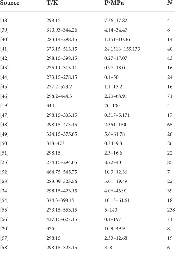
TABLE A3. CH4 solubility in water database.
Keywords: solubility, CO2, gas invasion, multiphase flow, gas volume fraction
Citation: He H, Sun B, Sun X, Li X and Shan Z (2022) Study on flow characteristics of natural gas containing CO2 invading wellbore during drilling. Front. Phys. 10:1028671. doi: 10.3389/fphy.2022.1028671
Received: 26 August 2022; Accepted: 20 September 2022;
Published: 07 October 2022.
Edited by:
Weiqi Fu, China University of Mining and Technology, ChinaReviewed by:
Yuanhang Chen, Louisiana State University, United StatesCopyright © 2022 He, Sun, Sun, Li and Shan. This is an open-access article distributed under the terms of the Creative Commons Attribution License (CC BY). The use, distribution or reproduction in other forums is permitted, provided the original author(s) and the copyright owner(s) are credited and that the original publication in this journal is cited, in accordance with accepted academic practice. No use, distribution or reproduction is permitted which does not comply with these terms.
*Correspondence: Baojiang Sun, c3VuYmoxMTI4QHZpcC4xMjYuY29t
Disclaimer: All claims expressed in this article are solely those of the authors and do not necessarily represent those of their affiliated organizations, or those of the publisher, the editors and the reviewers. Any product that may be evaluated in this article or claim that may be made by its manufacturer is not guaranteed or endorsed by the publisher.
Research integrity at Frontiers
Learn more about the work of our research integrity team to safeguard the quality of each article we publish.